Sage Journals: Discover world-class research

Abstract

Objective

Although the growing prevalence of obesity has led to an increased reliance on health-tracking apps for weight management, their effectiveness remains limited owing to missing data and irregular sampling of user-reported records. These issues highlight the need for more sophisticated predictive models to address real-world data limitations and offer personalized interventions. This study developed a gated recurrent unit–ordinary differential equation (GRU–ODE)–Bayes-based deep learning framework to predict successful weight loss using real-world lifelog data.

Methods

We analyzed a retrospective cohort of Noom Coach users, who logged data at least twice a month for six months between 2012 and 2014. We included demographic and self-monitoring variables, with weight loss ≥5% in three months as the primary outcome. We evaluated the model performance using the area under the receiver operating characteristic curve (ROC AUC) and precision–recall curve (PRC AUC).

Results

This study utilized a large-scale dataset (N = 34,322) that was subdivided into training (N = 24,292), validation (N = 6074), and test sets (N = 3375). Participants who frequently logged their weight, exercise, meals, and snacks were more likely to achieve weight loss. The model achieved an ROC AUC of 0.830 [95% confidence interval 0.819–0.840] and PRC AUC of 0.727 [0.707–0.746] in the validation set, and an ROC AUC of 0.821 [0.806–0.835] and PRC AUC of 0.717 [0.689–0.744] in the test set, using only the first four weeks of lifelog data. Early weight change and initial weight were the most important features as determined by the integrated gradients.

Conclusion

The proposed model predicted early outcomes in weight management and might contribute to developing effective intervention methods for participants at risk of failure and reducing the burden of frequent self-reporting.

Keywords

Lifestyle weight loss lifelog prediction deep learning neural ordinary differential equation

Introduction

The obesity epidemic continues to impose substantial public health and economic burdens on affected individuals and societies worldwide.¹ In recent years, health-tracking apps targeting weight management have emerged as an approachable and promising way to alleviate obesity-related health problems.² Combined with principled behavioral intervention methods, these apps have shown considerable efficacy in promoting lifestyle changes and aiding weight control.^3,4

A lifelog combines data from multiple sources to create a record from which individuals can retrieve information about themselves and their environment.⁵ Recently, various state-of-the-art (SOTA) methods have been explored for predicting successful weight loss outcomes using lifelog and self-reported data from mobile apps and wearable devices. Biehl et al. evaluated multiple traditional machine learning (ML) techniques and found logistic regression particularly effective, reaching up to 91% accuracy in predicting long-term weight-change categories based on longitudinal weight logs from participants in a digital coaching program.⁶ Furthermore, wearable device data have been integrated with biomarkers using gradient boosting models, as shown by Romero-Tapiador et al., which successfully predicted short-term weight-loss outcomes (AUC 84.4%),⁷ emphasizing the value of multimodal data sources for personalized weight management predictions.

However, developing effective ML models from lifelog data remains challenging because user-reported weight-related records are noisy and incomplete. Many existing ML-based prediction algorithms often fail to adequately address these challenges related to missing data^8,9 by assuming complete records with regular time intervals, thereby significantly limiting their applicability in real-world settings. Recent critiques have highlighted that missing data in health-related ML studies are frequently ignored or inadequately addressed, resulting in biased predictions and the loss of critical information.^8,9 Although imputation may be a possible solution, naively imputing the missing records of non-reporters with those from frequent reporters is likely to induce unreliable results due to user heterogeneity. Furthermore, different features may require distinct imputation strategies. For instance, many individuals tend to show a relatively high record frequency for exercise while exhibiting more reluctance to regularly log their weight measurements, possibly due to psychological barriers such as shame.¹⁰ Therefore, devising an optimal imputation strategy for weight-related lifelog data can be cumbersome and requires additional knowledge about the data-generating process.

Despite these challenges, incomplete lifelog data with distinctive patterns of missingness may reveal valuable information regarding user characteristics and behaviors. Harvey et al. reported that frequent self-reporting is significantly associated with successful weight loss. Conversely, patterns of infrequent or missing records (nonreporting) could also serve as useful diagnostic indicators for predicting individual weight loss outcomes.¹¹ Groenwold highlighted that the potential informational value inherent in the reasons behind missing data—such as intentional non-reporting because of stigma or unintentional omission—is typically overlooked, even though such missingness can reflect meaningful behavioral patterns.¹² Similarly, Braem et al. demonstrated that missing data statistics from wearable sensors can provide causal insights into why data loss occurs and how it relates to user engagement.¹³ Hence, these findings suggest that explicitly incorporating such patterns and reasons underlying missing data into predictive models may enhance their accuracy and interpretability in weight management applications.

A key motivation for this study is the need for more sophisticated predictive models that can handle real-world data and the many common challenges in health-tracking app data, including irregularly sampled time series data and data sets with missing values. The current study presents a novel framework for the early prediction of successful weight loss, specifically designed to handle the issues regarding real-world lifelog data. To demonstrate the validity and efficacy of our framework in a real-world setting, we used the lifelog data collected in approximately 80 countries using a widely used weight management app.¹⁴ We examined whether our model could predict targeted weight loss (that is, losing ≥5% of weight in 3 months).

To this end, we implemented a deep learning (DL) model derived from neural ordinary differential equations (ODEs),¹⁵ a recently suggested class of DL models that has shown promising outcomes for healthcare applications,¹⁶ particularly for irregularly sampled (i.e. collected at varying intervals) observations. For example, multimodal neural ODEs have successfully generated synthetic patient-level datasets that closely resemble real-world data on marginal distributions and correlations between variables.¹⁶ In addition, for Parkinson's disease, machine learning classifiers trained on synthetic data with multimodal neural ODEs had an area under the receiver operator curve (AUC) value similar to that of classifiers trained on real-world data (0.97 for both real and synthetic data).¹⁶ By using neural networks to parameterize the time derivative of the hidden state and integrate it across time, neural ODEs model the dynamics of interest in a continuous-time manner,¹⁷ and thus, can effectively handle irregularly sampled time-series, including weight-related lifelog data. Specifically, we adopted gated recurrent unit–ordinary differential equation (GRU–ODE)–Bayes as our basis model.¹⁸ GRU–ODE–Bayes consists of two modules, namely GRU–ODE and GRU–Bayes. The former is a continuous-time version of a GRU based on a neural ODE, while the latter is a Bayesian update network that updates the hidden state during actual observations.

Methods

Participants and study design

We conducted a retrospective cohort study using data collected from Noom Coach (Noom Inc., New York, NY, USA) users between October 10, 2012, and April 9, 2014. The specifics of the intervention with Noom coach are described in preceding studies.^14,19 The dataset included demographic and lifelog data, such as current body weight, daily food intake, amount of exercise, and patterns of app usage.

Among the app users, only those who had logged in and recorded lifelog data at least twice per month for six consecutive months were included in the current study. We also excluded users who said they were 42 years old, which is the default age set in the app, because many users do not change their default age to their actual age when using the app. The detailed inclusion and exclusion criteria for the entire dataset used in the current study are described in a previous study,¹⁴ and a total of 34,322 users were included in the resulting dataset.

Variables

We utilized both the baseline user information (age, sex, height, country, date of the first use, and use of the pro version of the app) and time-variant variables on weight, diet (calorie intakes from breakfast/lunch/dinner and morning/afternoon/evening snacks), and exercise (calorie expenditure from exercise), which were summarized on a daily basis. A preceding study described how diet and exercise are recorded and converted into calorie intake and expenditure in the Noom Coach app.¹⁴ We created additional variables, such as the body mass index (BMI) and the amount of weight change between the first and second weeks, based on the original variables. App users self-reported their body weight, dietary intake, and exercise habits daily, and these data were included as variables in our analysis.

Definition of outcome of successful weight loss

The primary outcome was a binary objective variable indicating whether the participants achieved effective weight loss, defined as a loss of at least 5% of their baseline body weight at the three-month endpoint. An initial weight loss of 5% or more in the first three months is known to be a strong predictor of long-term weight loss success. Thus, as in previous clinical studies, we used three months as the endpoint to assess the effectiveness of weight loss.^20–25

Data preprocessing

We performed preprocessing and transformation of the dataset, originally collected in an earlier study investigating the effects of a weight management app,¹⁴ to remove outliers and to prepare it for modeling. We subdivided the resulting dataset (N = 34,322) into training (N = 24,292), validation (N = 6074), and test sets (N = 3375) using stratified sampling to maintain the ratio of the success and failure groups. We first divided the entire dataset into a train-validation set and a test set in a 9:1 ratio. Then, we separated the training and validation sets in the same ratio.

To account for the high variance in user-recorded values, we excluded users with the top 1% of variance in weight as well as those with the top and bottom 0.5% of variances in other variables. Outliers included improbable daily weight fluctuations in self-reported weight data (e.g. extreme fluctuations, such as gaining or losing 10 kg per day). To detect these outliers, we applied an interquartile range analysis and conducted an additional manual inspection to capture unrealistic and rapid weight changes that may not have been identified solely by statistical thresholds. All baseline and time-varying feature values were scaled using the min-max scaling method.²⁶

Model development and validation

The baseline (i.e. static) features included some of the baseline user information (age, sex, an indicator variable denoting whether each individual had ever used the Noom Coach app's pro version, and the users’mpa#rsquo;' country of living). Initial weight change measured between the first two weeks was also included as a baseline feature to represent early-stage user characteristics before further observations. We constructed the initial hidden states of the model using the baseline variables. We encoded categorical baseline features using Catboost,²⁷ a method that has proven its effectiveness in various ML tasks, particularly for the treatment of high-cardinality categorical and heterogeneous features.²⁸ We then used the baseline covariate map obtained by encoding the baseline variables as the initial hidden state of the neural ODE-based model.

The time-varying (i.e. dynamic) features, which were the main inputs of the GRU–ODE–Bayes model, included the reported values for the time-variant variables: weight, calorie expenditure through exercise, and calorie intakes from regular meals (breakfast/lunch/dinner) and snacks (morning/afternoon/evening). In the case of weight, changes recorded after the initial two weeks were treated as time-varying features. For the GRU–ODE–Bayes model, a mask indicating whether each feature was observed (i.e. whether the user reported each feature) was created and used as an additional input, along with the actual feature values.

We carried out all our experiments in a single GPU setting using a Tesla P40. The GRU–ODE–Bayes model was implemented with PyTorch and trained for 50 epochs, with a batch size of 128, learning rate of 0.001, and weight decay of 0.1, with an AdamP optimizer.²⁹ We chose the hyperparameters based on a preliminary hyperparameter search.

Performance metrics

We assessed the respective performances of the model in different settings using the area under the receiver operating characteristic curve of sensitivity and specificity (ROC AUC) and area under the precision–recall curve (ROC PRC). To investigate the effect of data availability, we examined model performances with data from different time spans (the first 2, 3, and 4 weeks of app usage, respectively).

Interpretability analysis

To further investigate the features contributing to the model's decision, we conducted analyses on interpretability using a post-hoc model-agnostic method called integrated gradients (IG), implemented via the Captum library.^30,31 IG provides feature attribution by integrating the gradients of the model's output with respect to each input feature along a linear path from a predefined baseline (typically a zero or neutral input) to the actual input sample. This approach quantifies the influence of each feature on the model's prediction by accumulating sensitivity information across that path, thereby offering a more robust attribution compared with standard gradient-based methods. Using IG, we separately assessed the respective contributions of the baseline and time-varying features on the best-performing GRU–ODE–Bayes model.

We created separate all-zero baselines for the baseline and time-varying features to represent the condition of insufficient reporting. In this setting, an all-zero input does not correspond to an actual user trajectory but instead represents a counterfactual condition where the model receives no informative weight or lifestyle input. Because the trained model has internalized population-level patterns of weight change during training, it can still generate a baseline prediction even under this uninformed condition. This counterfactual baseline provides a neutral starting point for attribution analysis, enabling IG to quantify how much each observed feature contributes to shifting the model's prediction from the uninformed baseline toward the prediction based on actual recorded data. We then used these baselines in combination with the corresponding real-data inputs to calculate the IG results.

Statistical analysis

All statistical analyses were conducted using Python 3.8/3.10 with NumPy, Pandas, SciPy, Scikit-learn, TorchMetrics, and Statsmodels for data processing and statistical computation. For descriptive statistics involving proportions (i.e. feature reporting frequencies), 95% confidence intervals were calculated using the Wilson interval via the proportion_confint function from Statsmodels. The Wilson interval was selected over the normal approximation due to its superior coverage properties for proportions near 0 or 1. Model performance metrics (ROC AUC and PRC AUC) were accompanied by 95% confidence intervals estimated via nonparametric bootstrapping, implemented using the BootStrapper module from TorchMetrics, with each interval based on 5000 bootstrap resamples generated with multinomial sampling.

Ethics statement

This preceding study was conducted in accordance with the Declaration of Helsinki guidelines, as well as the privacy policy of Noom Inc.¹⁴ The study was approved by the Kyung Hee University Hospital Institutional Review Board (KMC IRB 1435-04), upon confirmation of the absence of privacy leakage risk. The KMC IRB waived the requirement for informed consent from the participants due to the retrospective design of the preceding study. This study followed the guidelines outlined in the transparent reporting of a multivariate prediction model for individual prognosis or diagnosis (TRIPOD) statement.

Results

Dataset and user characteristics

Table 1 shows the baseline user characteristics for the training and test sets. The time-varying (i.e. dynamic) features included lifelog data on weight, calorie expenditure through exercise, and calorie intakes from regular meals and snacks. We treated age, sex, usage of the app's pro version, country of living, and early weight change within the first two weeks as baseline (i.e. static) features. A summary of missing data rates is provided in Supplemental Table S1, indicating that dietary and exercise variables exhibited high proportions of missing data.

Table 1.

Baseline characteristics of the participants assigned to the training, validation, and test sets.

	Training set		Validation set		Test set
	Success	Failure	Success	Failure	Success	Failure
Number (%)	9097 (37.5)	15,195 (62.6)	2275 (37.5)	3799 (62.6)	1264 (37.5)	2111 (62.6)
Age, years	35.3 ± 10.5	34.2 ± 10.6	35.0 ± 10.4	34.2 ± 10.5	34.6 ± 10.2	34.1 ± 10.7
Female	6484 (71.3)	12,170 (80.1)	1618 (71.1)	3032 (79.8)	896 (70.9)	1706 (80.8)
Weight (kg)	83.9 ± 20.1	78.4 ± 20.7	83.8 ± 19.9	78.5 ± 20.6	85.1 ± 20.5	78.3 ± 20.5
BMI (kg/m²)	29.4 ± 5.9	27.9 ± 6.5	29.4 ± 5.9	28.0 ± 6.3	29.7 ± 6.1	27.9 ± 6.4
Obesity class^a
Underweight	0.2%	0.7%	0.1%	1.0%	0.3%	1.0%
Normal	20.9%	33.7%	20.4%	33.4%	18.8%	33.7%
Overweight	33.1%	29.3%	34.0%	29.1%	33.3%	28.1%
Obesity Class I	20.7%	15.5%	21.4%	15.7%	21.8%	16.3%
Obesity Class II	8.6%	6.5%	8.0%	6.3%	8.3%	7.0%
Obesity Class III	5.2%	4.8%	4.8%	4.8%	5.8%	4.3%

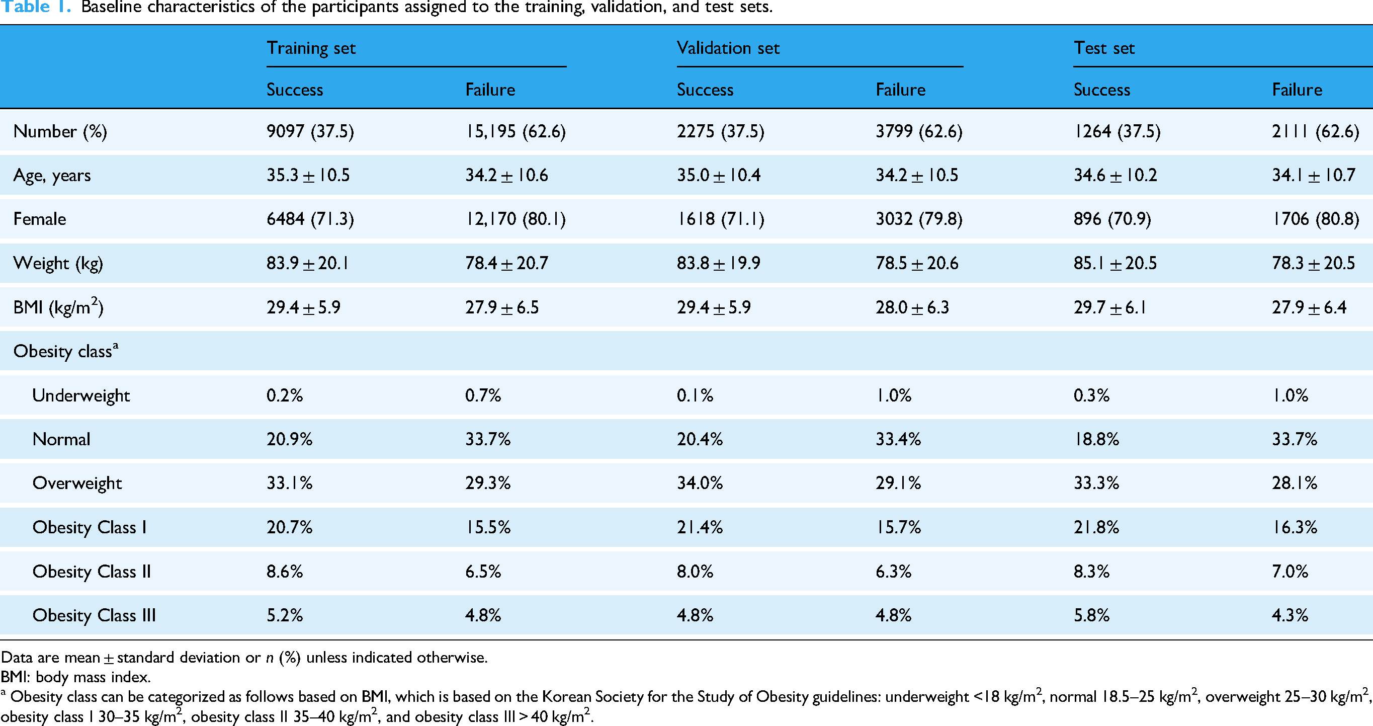
Data are mean ± standard deviation or n (%) unless indicated otherwise.

BMI: body mass index.

^a Obesity class can be categorized as follows based on BMI, which is based on the Korean Society for the Study of Obesity guidelines: underweight <18 kg/m², normal 18.5–25 kg/m², overweight 25–30 kg/m², obesity class I 30–35 kg/m², obesity class II 35–40 kg/m², and obesity class III > 40 kg/m².

Figure 1 illustrates the weekly recorded frequencies of the time-varying features (weight, exercise, meals, and snacks) over a 24-week period for the successful and unsuccessful groups. Across all time-varying features, users who successfully achieved at least 5% weight loss by three months showed consistently higher logging frequencies than those who did not. Specifically, the frequency of meal recording was the highest among the four features in both groups, whereas snack logging had the lowest overall frequency. Additionally, although the record frequency for all features gradually decreased over time in both groups, the successful group maintained consistently higher engagement levels throughout the observation period than the unsuccessful group.

Figure 1.

Weekly recorded frequencies of time-varying features during the six months of app usage: (a) weight, (b) exercise, (c) meals, and (d) snacks. The blue and red solid lines indicate the observations from the success and failure groups, respectively. The shaded regions outlined with gray dotted lines indicate the 95% confidence intervals.

Model structure and performance

Figure 2 displays the schematic overview of the proposed GRU–ODE–Bayes framework. At baseline (t = 0), baseline features were embedded to initialize the hidden state, representing the individual's initial condition. As observations of time-varying features became available, the hidden state was continuously updated in two steps: (1) between observations, the hidden state evolved smoothly according to an ODE solver; and (2) upon each new observation, a GRU update was applied to incorporate the newly observed data. Ultimately, the model was utilized to predict the outcome of achieving significant weight loss (≥5% of baseline weight) at the three-month endpoint.

Figure 2.

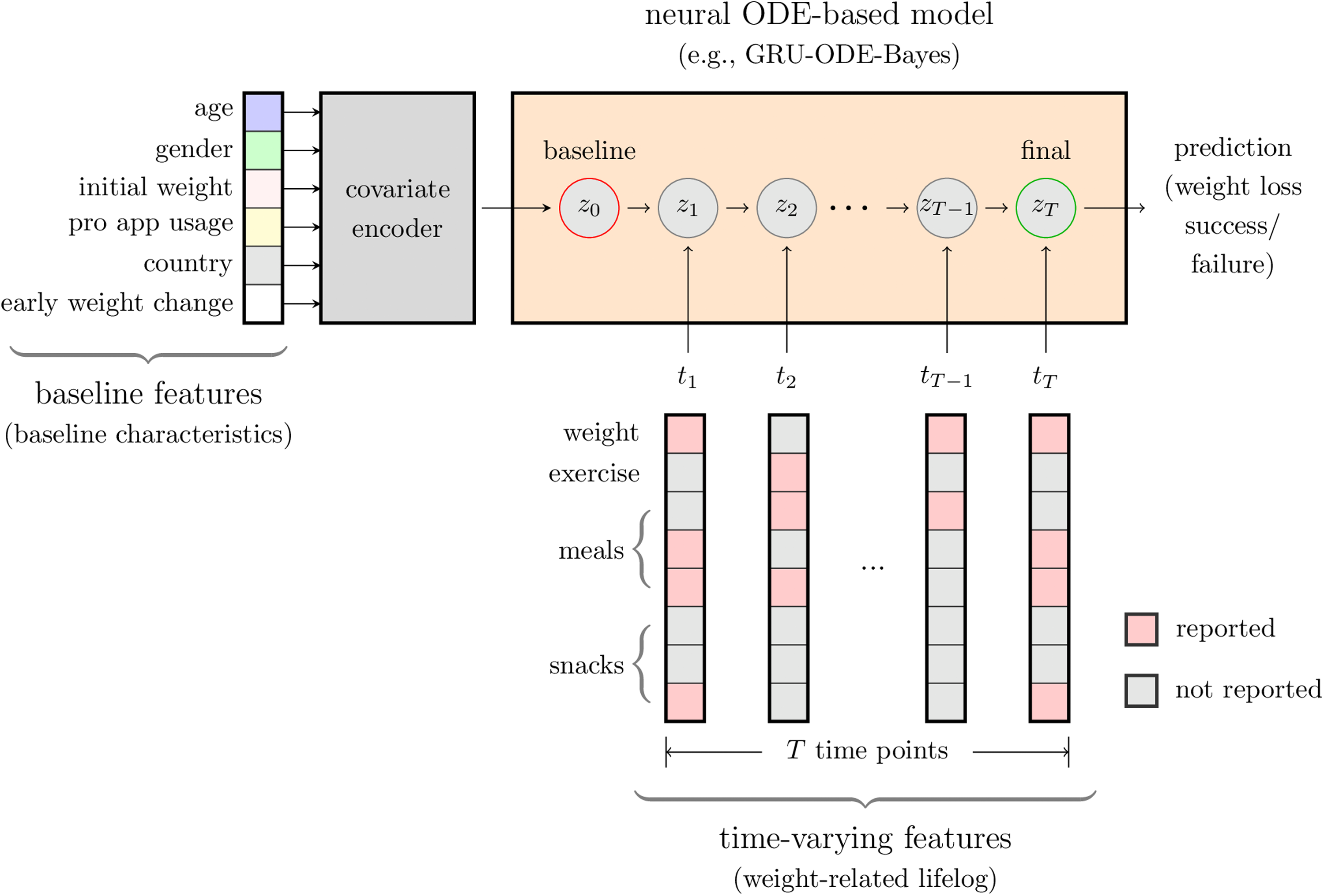
Schematic overview of the proposed GRU–ODE–Bayes framework for the early prediction of successful weight loss. Baseline features included age, gender, initial weight, pro-app usage, country, and early weight changes. Time-varying features (weight-related lifelog data) comprised user-reported values for weight, exercise, meals, and snacks recorded at irregular time intervals (time points t₁, t₂, …, t_T). The resulting baseline covariate map was used to initialize the hidden state of the model (z₀). The model integrates time-varying features using masks that indicate reported and unreported values to update the hidden states over time. As observations of time-varying features became available, the hidden state was continuously updated in two steps: (1) between observations, the hidden state evolved smoothly according to an ODE solver, and (2) upon each new observation, a GRU update was applied to incorporate the newly observed data. Ultimately, the model predicted whether the user would achieve significant weight loss (≥5%) at three months.

The GRU–ODE–Bayes model displayed a significant performance, achieving an ROC AUC of over 0.8 and a PRC AUC of over 0.7 on the validation and test sets using data from the first four weeks (Table 2). The performance of the model tended to improve as the observation period increased, primarily because a longer time span provided more available data points for the model to learn from (Figure 3). This improvement indicates that capturing more extensive and richer initial data enables the model to learn more precise individual user behavior patterns, thus leading to enhanced prediction accuracy. Practically, this highlights the importance of ensuring consistent user engagement and regular data reporting, particularly during the early phases of participation, to improve predictive accuracy within the three-month period assessed in this study.

Figure 3.

Performance of the GRU–ODE–Bayes model. (a) ROC AUC curves for the data from the first 2, 3, and 4 weeks of app usage. (b) ROC PRC curves for the data from the first 2, 3, and 4 weeks of app usage. ROC AUC, areas under the receiver operator characteristic curve of sensitivity and specificity; ROC PRC, receiver operator characteristic curve of precision and recall.

Table 2.

Performance of the GRU–ODE–Bayes model.

	Validation set		Test set
	ROC AUC	PRC AUC	ROC AUC	PRC AUC
First 2 weeks	0.775 (0.763–0.787)	0.661 (0.640–0.682)	0.770 (0.753–0.786)	0.651 (0.623–0.679)
First 3 weeks	0.800 (0.789–0.811)	0.694 (0.673–0.714)	0.795 (0.779–0.810)	0.690 (0.663–0.717)
First 4 weeks	0.830 (0.819–0.840)	0.727 (0.707–0.746)	0.821 (0.806–0.835)	0.717 (0.689–0.744)

Values in parentheses denote 95% confidence intervals obtained from 5000 bootstrapping iterations.

ROC AUC: area under the receiver operator characteristic curve of sensitivity and specificity; PRC AUC: area under the precision–recall curve.

Interpretability outcomes: Feature importance analysis using IGs

Figure 4 shows the results of the feature importance analysis using IG. Using the heatmap intensity,^32,33 which represents the magnitude of each feature's contribution, we visualized the IG values for the baseline and time-varying features influencing successful weight loss. We used the mean absolute IG magnitude to summarize each feature's contribution across participants (Figure 4(a) and 4(c)), while we showed individual-level IG patterns for selected participants (Figure 4(b) and 4(d)).

Figure 4.

Results from the interpretability analysis using Integrated Gradients (IGs). (a) Mean IG values for the time-varying features. (b) IG values from a single participant for the time-varying features. (c) Mean IG values for the baseline features. (d) IG values from three participants for the baseline features. The IG values from the best-performing GRU–ODE–Bayes model with the first-2-week test set are shown. The color darkens with the increasing absolute value of IG.

Across participants, the largest absolute IG values (≥0.01) were observed for features reflecting weight and monitoring behavior, including (i) baseline: early weight change and initial weight, and (ii) time-varying: the number of weight records per week, particularly during the initial week. This notable influence of weight-related features likely reflected their direct association with the target. Other variables showed much smaller absolute IG values, suggesting comparatively limited impact on the model's predictions.

Discussion

This study utilized a neural ODE-related model for weight management prediction using real-world data. Specifically, we adopted the GRU–ODE–Bayes model. Unlike traditional discrete-time models, GRU–ODE–Bayes continuously updates its hidden states whenever new data points are observed, thereby effectively handling irregularly timed data entries. This capability allows the model to directly leverage both the presence and timing of user-reported lifelog events, thus fully utilizing the dynamic and sparse nature of real-world lifelog datasets to enhance the predictive accuracy and robustness. Our main findings indicate the proposed model's effectiveness in predicting whether participants will achieve significant weight loss (≥5% of baseline body weight) at three months of application usage, using only the first few weeks of irregularly sampled lifelog data. The proposed model exhibited consistent predictive performance when using lifelog data from the first four weeks (ROC AUC and PRC AUC, 0.830 and 0.727 in the validation set and 0.821 and 0.717 in the test set, respectively). In the IG analysis, early weight change and initial weight were the most influential factors in predicting weight loss success within the three-month horizon.

Previously reported SOTA models have demonstrated strong predictive performance using fully observed or regularly sampled datasets. DL approaches, such as long short-term memory networks, have successfully predicted childhood obesity outcomes with temporal data, achieving AUC scores ranging from 0.80 to 0.92.³⁴ Traditional ML methods, including random forests, support vector machines, and recurrent neural networks (RNNs), have also effectively predicted weight loss outcomes by utilizing static or fully observed time series data.^35,36 However, these models often rely on data completeness and regularity, which pose significant limitations when applied to real-world scenarios involving irregularly timed or missing observations. Consequently, their performance and applicability can be degraded when faced with realistic lifelog data characterized by frequent gaps and inconsistent recording intervals.

In addition, Shahabi et al. developed a random forest classifier leveraging initial weight-loss patterns and baseline demographics, achieving high predictive performance (AUROC 84.5%) in identifying successful weight loss at six months.³⁷ Although their model achieved strong performance, it required relatively complete datasets. In contrast, our study highlights that comparable predictive accuracy can be obtained within the first four weeks of app use, even with irregular and incomplete records. Importantly, our GRU–ODE–Bayes framework was developed to operate under conditions of irregular sampling and frequent missing values, which are common in real-world app usage. Despite these challenges, the predictive accuracy achieved in our study was of a similar magnitude to that reported by Shahabi et al., underscoring that reliable predictions can be obtained even when data are incomplete or inconsistently recorded. Similarly, Kim et al. implemented an interpretable RNN model using daily lifelog data (weight, diet, exercise logs) from a commercial app,³⁶ demonstrating accurate weekly predictions and providing interpretable behavioral insights but still relying on consistent reporting. In contrast, the GRU–ODE–Bayes model explicitly addresses these critical limitations by inherently accommodating irregular sampling intervals and directly utilizing the informative value of missingness patterns without relying on imputation methods that could introduce biases. This capability stems from its continuous-time design and Bayesian update mechanism (GRU–Bayes module), which dynamically integrates new observations and effectively manages data variability. Therefore, our GRU–ODE–Bayes approach not only achieves competitive predictive accuracy, but also provides enhanced robustness and practical applicability in realistic weight management prediction settings.

This study highlights a significant strength in demonstrating that the proportion of participants who successfully lost weight increased with the frequency with which the participants recorded lifelog data on weight, exercise, and calorie intake and expenditure from food. This phenomenon can be understood in the framework of self-regulation theory, which describes behavior change as a cyclical process of self-monitoring, evaluating progress against personal goals, and adjusting behavior accordingly.³⁸ In this framework, frequent self-monitoring provides essential feedback that helps individuals sustain motivation and maintain adherence to behavioral goals. Similar findings were reported in the Look AHEAD study, where participants in the intensive lifestyle intervention group who frequently measured their body weight and consistently monitored dietary intake and physical activity showed significantly better long-term weight loss outcomes compared to those who did not regularly engage in these self-monitoring behaviors.³⁹ Specifically, participants who frequently engaged in self-weighing, dietary monitoring, and regular physical activity demonstrated greater weight loss and sustained adherence to lifestyle changes over an extended period of 8 years.³⁹ Additional research in behavioral treatment of obesity and lifestyle modification programs has consistently shown that self-monitoring is a cornerstone strategy for achieving and maintaining weight loss.^40,41 Consistent with these findings, our study emphasizes that frequent self-reporting behaviors—reflecting sustained adherence and engagement—are strong predictors of successful weight loss. The ability of the GRU–ODE–Bayes model to leverage self-reporting behaviors enables it to identify individuals who are likely to succeed or struggle in their weight-loss efforts early in the intervention. This predictive capacity could support the development of more timely and tailored behavioral support within personalized weight management programs.

We applied explainable artificial intelligence techniques to explore how both baseline and time-varying features contributed to the model's predictions. The attribution analysis revealed that early weight change and initial weight had the strongest influence, which is consistent with prior literature identifying early weight loss as a key prognostic marker of long-term outcomes.^42,43 In addition, although many variables were included in the dataset, a large proportion were self-reported and subject to substantial missingness—for example, dietary and exercise records were often incomplete. As a result, the effective information available to the model was much smaller than the raw number of features might suggest. In this context, interpretability provides supplementary value by showing that the model relied on clinically meaningful features despite these constraints.

There also exists room for improvement in the implementation of IG for model interpretability. For instance, augmenting IG with a temporal saliency rescaling approach can enhance the attribution of feature importance over time.⁴⁴ In addition, developing better baselines for weight prediction settings may lead to more reliable feature attribution. The IG values for the time-varying features also revealed that the observed features were assigned greater importance than the unobserved features, suggesting that the influence of incoming observations was indeed reflected in the model. Such methodological enhancements in IG could significantly improve its validity and efficacy, facilitating more insightful and useful interpretability analyses in future artificial intelligence (AI)-driven health application research.

The current study had several limitations. The study population included generally consistent app users, with a minimum usage duration of 180 days. As a result, the current findings may not generalize well to a population including many early churn users. We thus plan to conduct future studies featuring a wider range of app users. Second, although the GRU–ODE–Bayes model effectively handled irregularly sampled data, the study relied on self-reported data, which can be prone to inaccuracy. Memory recall issues or social desirability biases can cause users to underreport or overreport certain behaviors, such as calorie intake or exercise frequency. Moreover, reliance on user-reported weight, which is the main outcome of the study, can affect the accuracy of the results owing to intentional or unintentional misreporting, potentially affecting the reliability of our model's predictions. Third, we trained and validated the model using data from a single weight management application, Noom Coach, which may have limited its external validity. The generalizability of our model to other populations, settings, and weight-management programs remains uncertain. Future studies should validate this model using data from diverse sources to ensure its broader applicability. Fourth, since we included only participants who logged data at least twice per month for six consecutive months, our findings might have limited generalizability and could omit insights into behaviors and outcomes among less-engaged users.

Additionally, there are limitations related to the design and scope of the prediction. False positives can arise when participants show early weight loss, often due to water loss, or when they intensively self-report in the initial months, but stop logging data afterward. This leads the model to overestimate its success even if individuals regain this weight later. Conversely, false negatives may occur when weight loss is initially slow but accelerates towards the end of the three months, causing the model to underestimate the outcome based on earlier data. Both false positives and false negatives pose a risk to the accuracy of the model by either promoting ineffective interventions or missing opportunities to support participants who are likely to succeed. In addition, in the previous literature, the operational definition of early weight loss tended to vary according to study purposes and schemes. Focusing only on a three-month predicted time point is limited in addressing the sustainability of weight loss. Our study was designed with the primary aim of evaluating whether short-term outcomes could be predicted using only the first few weeks of lifelog data, reflecting the practical and clinical importance of early risk stratification. In real-world settings, many users do not engage with weight management apps for extended periods, partly because of subscription costs, and early prediction can provide timely guidance on whether continued engagement is likely to be beneficial. Nevertheless, by restricting the prediction horizon to three months, our findings may not generalize to longer-term outcomes such as weight loss at six months or beyond. Finally, we excluded users reporting their age as 42 years, the default age set in the app, which limited the ability to explain weight loss in younger participants under 42 years old.

Conclusion

In conclusion, this study demonstrates the feasibility of applying the GRU–ODE–Bayes framework to predict weight management outcomes at three months using lifelog data that are incomplete and irregularly sampled, a common scenario in real-world settings. The methodological contribution of our work lies in showing that this approach can accommodate noisy self-reported variables without relying on imputation, while still identifying clinically meaningful features such as early weight change and initial weight. Although early prediction has potential clinical utility, our findings should be interpreted within the context of the three-month horizon assessed. In future studies, evaluating the framework in relation to longer-term outcomes will be crucial for improving the robustness and applicability of predictive models in weight management.

Supplemental Material

sj-docx-1-dhj-10.1177_20552076251406656 - Supplemental material for A deep learning-based early prediction framework for weight management using real-world lifelog data: GRU–ODE–Bayes model development and validation study

Supplemental material, sj-docx-1-dhj-10.1177_20552076251406656 for A deep learning-based early prediction framework for weight management using real-world lifelog data: GRU–ODE–Bayes model development and validation study by Yera Choi, Hyunji Sang, Sunyoung Kim, Haanju Yoo and Sang Youl Rhee in DIGITAL HEALTH

Supplemental Material

sj-docx-2-dhj-10.1177_20552076251406656 - Supplemental material for A deep learning-based early prediction framework for weight management using real-world lifelog data: GRU–ODE–Bayes model development and validation study

Supplemental material, sj-docx-2-dhj-10.1177_20552076251406656 for A deep learning-based early prediction framework for weight management using real-world lifelog data: GRU–ODE–Bayes model development and validation study by Yera Choi, Hyunji Sang, Sunyoung Kim, Haanju Yoo and Sang Youl Rhee in DIGITAL HEALTH

Footnotes

Acknowledgments

The authors would like to thank Prof. Emeritus Young Seol Kim from Kyung Hee University for his exceptional teaching and inspiration.

ORCID iDs

Yera Choi

Hyunji Sang

Sunyoung Kim

Haanju Yoo

Sang Youl Rhee

Ethical considerations

The study was approved by the Kyung Hee University Hospital Institutional Review Board (KMC IRB 1435-04), upon confirmation of the absence of privacy leakage risk. The requirement of informed consent from the participants was waived by the KMC IRB due to the retrospective design of the preceding study.

Contributorship

Y.C., S.Y.R, and H.Y. conceptualized the study; Y.C. and H.Y. conceived the experiments; and Y.C. carried out the experiments and analyzed the data. S.K. and S.Y.R. advised on the clinical aspects of the study. Y.C. and H.S. wrote the original draft of the manuscript. All authors were involved in writing the final version of the manuscript and provided final approval for the submitted and published versions.

Funding

The authors disclosed receipt of the following financial support for the research, authorship, and/or publication of this article: This work was supported by the Technology Innovation Program (or Industrial Strategic Technology Development Program) (RS-2025-07892971, AI-Based Development of the BEACON (Biosignal Emergency Advanced Critical Observation Network) System for Real-Time Monitoring and Early Warning of Critical Trauma Patients' Vital Signs) funded by the Ministry of Trade, Industry & Resources (MOTIR, Korea).

Declaration of conflicting interests

The authors declared the following potential conflicts of interest with respect to the research, authorship, and/or publication of this article: YC and HY with NAVER Digital Healthcare LAB; and SYR with Kyung Hee University Medical Center.

Data availability

The data that support the findings of the current study are available from Noom Inc. However, restrictions apply to the availability of these data, which were used under license for the current study, and thus, are not publicly available. Data are, however, available from the corresponding authors upon reasonable request and with permission from Noom Inc.

Supplemental material

Supplemental material for this article is available online.

References

Bluher

. Obesity: global epidemiology and pathogenesis. Nat Rev Endocrinol 2019; 15: 288–298.

Beleigoli

Andrade

Cancado

, et al. Web-based digital health interventions for weight loss and lifestyle habit changes in overweight and obese adults: systematic review and meta-analysis. J Med Internet Res 2019; 21: e298.

Harvey-Berino

West

Krukowski

, et al. Internet delivered behavioral obesity treatment. Prev Med 2010; 51: 123–128.

Kim

Choi

. Digital therapeutics for obesity and eating-related problems. Endocrinol Metab (Seoul) 2021; 36: 220–228.

Jacquemard

Novitzky

O'Brolchain

, et al. Challenges and opportunities of lifelog technologies: a literature review and critical analysis. Sci Eng Ethics 2014; 20: 379–409.

Biehl

Venäläinen

Suojanen

, et al. Development and validation of a weight-loss predictor to assist weight loss management. Sci Rep 2023; 13: 20661.

Romero-Tapiador

Tolosana

Morales

, et al. Personalized weight loss management through wearable devices and artificial intelligence. arXiv preprint arXiv:240908700 2024.

Nijman

SWJ

Leeuwenberg

Beekers

, et al. Missing data is poorly handled and reported in prediction model studies using machine learning: a literature review. J Clin Epidemiol 2022; 142: 218–229.

Nguyen

Riegler

, et al. Multimodal missing data in healthcare: a comprehensive review and future directions. Comput Sci Rev 2025; 56: 100720.

10.

Frie

Hartmann-Boyce

Pilbeam

, et al. Analysing self-regulatory behaviours in response to daily weighing: a think-aloud study with follow-up interviews. Psychol Health 2020; 35: 16–35.

11.

Harvey

Krukowski

Priest

, et al. Log often, lose more: electronic dietary self-monitoring for weight loss. Obesity (Silver Spring) 2019; 27: 380–384.

12.

Groenwold

RHH

. Informative missingness in electronic health record systems: the curse of knowing. Diagn Progn Res 2020; 4: 8.

13.

Braem

CIR

Yavuz

Hermens

, et al. Missing data statistics provide causal insights into data loss in diabetes health monitoring by wearable sensors. Sensors (Basel) 2024; 24: 1526.

14.

Chin

Keum

Woo

, et al. Successful weight reduction and maintenance by using a smartphone application in those with overweight and obesity. Sci Rep 2016; 6: 34563.

15.

Chen

RTQ

Rubanova

Bettencourt

, et al. Neural ordinary differential equations. Adv Neural Inf Process Syst 2018; 31: 6572–6583.

16.

Wendland

Birkenbihl

Gomez-Freixa

, et al. Generation of realistic synthetic data using multimodal neural ordinary differential equations. NPJ Digit Med 2022; 5: 122.

17.

Greydanus

Lee

Fern

. Piecewise-constant neural ODEs. arXiv pre-print server 2021.

18.

De Brouwer

Simm

Arany

, et al. GRU-ODE-Bayes: continuous modeling of sporadically-observed time series. Adv Neural Inf Process Syst 2019; 32: 7377–7388.

19.

Han

Rhee

. Effectiveness of mobile health applications for 5% body weight reduction in obese and overweight adults. J Obes Metab Syndr 2021; 30: 354–364.

20.

Fujioka

O'Neil

Davies

, et al. Early weight loss with liraglutide 3.0 mg predicts 1-year weight loss and is associated with improvements in clinical markers. Obesity 2016; 24: 2278–2288.

21.

Fujioka

Plodkowski

O'Neil

, et al. The relationship between early weight loss and weight loss at 1 year with naltrexone ER/bupropion ER combination therapy. Int J Obes 2016; 40: 1369–1375.

22.

Halseth

Shan

Walsh

, et al. Method-of-use study of naltrexone sustained release (SR)/bupropion SR on body weight in individuals with obesity. Obesity 2017; 25: 338–345.

23.

Kheniser

Saxon

Kashyap

. Long-term weight loss strategies for obesity. J Clin Endocrinol Metab 2021; 106: 1854–1866.

24.

Finer

Ryan

Renz

, et al. Prediction of response to sibutramine therapy in obese non-diabetic and diabetic patients. Diab Obes Metab 2006; 8: 206–213.

25.

Rissanen

Lean

Rössner

, et al. Predictive value of early weight loss in obesity management with orlistat: an evidence-based assessment of prescribing guidelines. Int J Obes Relat Metab Disord 2003; 27: 103–109.

26.

Kulkarni

Joshua

, et al. Enhanced preprocessing approach using ensemble machine learning algorithms for detecting liver disease. Biomedicines 2023; 11: 581.

27.

Prokhorenkova

Gusev

Vorobev

, et al. Catboost: unbiased boosting with categorical features. In: Proceedings of the 32nd international conference on neural information processing systems, Montréal, Canada, 2018, pp.6639–6649: Curran Associates Inc.

28.

Hancock

Khoshgoftaar

. Catboost for big data: an interdisciplinary review. J Big Data 2020; 7: 94.

29.

Heo

Chun

, et al. Adamp: slowing down the slowdown for momentum optimizers on scale-invariant weights. arXiv preprint arXiv:200608217 2020.

30.

Kokhlikyan

Miglani

Martin

, et al. Captum: a unified and generic model interpretability library for pytorch. arXiv preprint arXiv:200907896 2020.

31.

Sundararajan

Taly

Yan

. Axiomatic attribution for deep networks. In: Doina

Yee Whye

(eds) Proceedings of the 34th international conference on machine learning. Sydney, Australia: PMLR, 2017, pp.3319–3328.

32.

Shirato

Andrienko

. Exploring and visualizing temporal relations in multivariate time series. Vis Inform 2023; 7: 57–72.

33.

Schlegel

Keim

. Time series model attribution visualizations as explanations. In: 2021 IEEE workshop on TRust and EXpertise in visual analytics (TREX), 24–25 October 2021, pp.27–31.

34.

Gupta

Phan

T-LT

Bunnell

, et al. Obesity prediction with EHR data: a deep learning approach with interpretable elements. ACM Trans Comput Healthcare 2022; 3: 32.

35.

Chatterjee

Gerdes

Martinez

. Identification of risk factors associated with obesity and overweight—a machine learning overview. Sensors 2020; 20: 2734.

36.

Kim

Park

. Interpretable conditional recurrent neural network for weight change prediction: algorithm development and validation study. JMIR Mhealth Uhealth 2021; 9: e22183.

37.

Shahabi

Battalio

Pfammatter

, et al. A machine-learned model for predicting weight loss success using weight change features early in treatment. npj Digit Med 2024; 7: 344.

38.

Kanfer

Goldstein

. Helping people change: a textbook of methods. New York, USA: Pergamon Press, 1991.

39.

Look

ARG

. Eight-year weight losses with an intensive lifestyle intervention: the look AHEAD study. Obesity (Silver Spring) 2014; 22: 5–13.

40.

Wadden

Tronieri

Butryn

. Lifestyle modification approaches for the treatment of obesity in adults. Am Psychol 2020; 75: 235–251.

41.

Burke

Wang

Sevick

. Self-monitoring in weight loss: a systematic review of the literature. J Am Diet Assoc 2011; 111: 92–102.

42.

El Masri

Itani

Kreidieh

, et al. Relationship between multiple weight cycles and early weight loss in patients with obesity: a longitudinal study. Eat Weight Disord 2021; 26: 2083–2087.

43.

Chopra

Malhotra

Ranjan

, et al. Predictors of successful weight loss outcomes amongst individuals with obesity undergoing lifestyle interventions: a systematic review. Obes Rev 2021; 22: e13148.

44.

Ismail

Gunady

Corrada Bravo

, et al. Benchmarking deep learning interpretability in time series predictions. Adv Neural Inf Process Syst 2020; 33: 6441–6452.

Supplementary Material

Please find the following supplemental material available below.

For Open Access articles published under a Creative Commons License, all supplemental material carries the same license as the article it is associated with.

For non-Open Access articles published, all supplemental material carries a non-exclusive license, and permission requests for re-use of supplemental material or any part of supplemental material shall be sent directly to the copyright owner as specified in the copyright notice associated with the article.

0.00 MB

0.01 MB

0.09 MB