Diaproteo: A supervised learning framework for early detection of diabetes mellitus based on proteomic profiles

Abstract

Diabetes mellitus (DM) is a chronic metabolic disease that affects millions of people worldwide, posing major health risks and financial challenges. Early diagnosis and treatment are essential for reducing complications and improving patient outcomes. This research explores the application of supervised algorithms to predict DM using a variety of datasets such as clinical features, genetic markers, and lifestyle variables. This study proposes novel approaches and evaluates prediction models with classic machine learning algorithms and cutting-edge deep learning architecture. Performance metrics (accuracy, precision, recall, F1 score) reveal that the Extra Trees model for the independent test and Convolutional Neural Network (CNN) for 10-fold cross-validation, achieving 91.52% accuracy with an F1 score of 0.91 (Extra Trees) and 87.03% accuracy with an F1 score of 84.82% (CNN). In addition, other evaluation indicators demonstrated that the Extra Trees algorithm outperformed others, achieving the highest accuracy on the independent test. Our study shows that machine learning and deep learning approaches may accurately predict DM, demonstrating the potential for early intervention and personalized healthcare strategies.

Introduction

Diabetes mellitus (DM), a chronic metabolic syndrome, is a global health concern affecting hundreds of millions of people, characterized by persistent hyperglycemia due to impaired insulin secretion, action, or both. The global prevalence of DM poses significant health, economic, and social challenges.^1,2 According to the World Health Organization, the international population of humans with diabetes has risen from 108 million in 1980 to 422 million in the year 2014, with further increases expected. Diabetes mellitus is a major global health crisis, with an estimated 463 million people affected, and this number is projected to rise to 700 million by the year 2045.^3–5 It affects millions of people worldwide, causing serious health issues such as heart disease, stroke, kidney disease, and loss of eyesight. Early detection and treatment are critical for preventing these risks. ⁶ Diabetes mellitus is categorized into three types: Type-1 diabetes occurs when the pancreas does not produce sufficient insulin. The immune system attacks insulin-producing cells, resulting in an insulin deficiency. Type-2 diabetes (T-2-D) is characterized by insulin resistance, which occurs when cells fail to respond to insulin signals. The pancreas eventually loses its ability to produce insulin. Gestational diabetes affects pregnant women who have no prior history. During pregnancy, their bodies are unable to maintain adequate blood sugar control. Conventional diabetes care methods rely heavily on clinical evaluations, tests performed in laboratories, and information provided by patients, which sometimes fail to adequately capture the disease's dynamic nature or patient diversity. Type 1 diabetes is caused by autoimmune destruction of pancreatic β-cells ⁷ in insulin deficiency. Type 2 diabetes is characterized by insulin resistance and relative insulin deficiency. Diabetes mellitus must be effectively managed and diagnosed early on to avoid serious health issues such as heart disease, neurological disorders, kidney failure, and retinal disease.^8,9

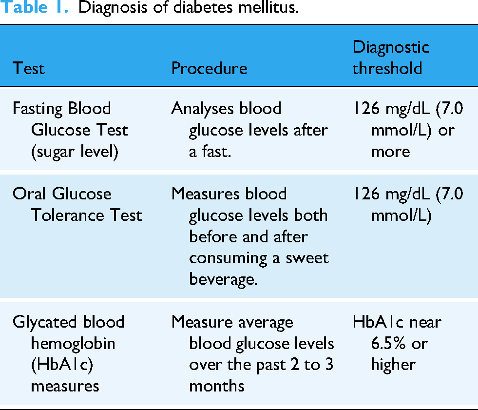
A Venn diagram depicted in Figure 1 signifies the two main types of DM, focusing on their key characteristics and differences. Type-1 diabetes is caused by an autoimmune disease that damages pancreatic cells, which leads to the complete lack or absence of insulin. Type-1 diabetics need insulin treatment for the rest of their lives to keep their blood glucose (sugar) levels under control. This condition is commonly diagnosed in childhood or adolescence, yet it can arise at any age. The precise reason is also unknown, but then environmental and genetic causes are thought to play a part. Type-2 diabetes is the most common type of DM and primarily caused by insulin resistance, which arises when the body cells fail to respond effectively to insulin. ¹⁰ Pancreatic β-cells will eventually produce insufficient insulin.^7,11,12 Obesity, lack of physical activity, and a poor diet are all frequently associated with type 2 diabetes. It usually occurs in adults, but the prevalence in children and adolescents is growing. Lifestyle changes, oral treatments, and, in rare cases, insulin treatment are utilized to control the disorder. Diabetic diagnostic methods serve as an overview (see Table 1) for understanding each method's procedure and purpose. The fasting blood glucose test analyzes levels after the patient has fasted for at least 7–8 h. approx. It is a basic and widely utilized test to identify diabetes and prediabetes. Diabetes is diagnosed when fasting blood glucose (sugar) levels are above 126 mg/dL (7.0 mmol/L) in two independent cases.^11–15 An oral glucose tolerance test analyzes the levels of sugar in the blood before and after two hours of drinking a carbohydrate-containing drink. It examines how well the body handles glucose. Diabetes is diagnosed by a glucose level of 200 mg/dL (11.1 mmol/L) or above after two hours. This test functions adequately to diagnose gestational diabetes. The glycated hemoglobin (HbA1c) Test defines common blood sugar levels over the previous 2–3 months by calculating the percentage of glycated hemoglobin in the blood. Diabetes has been diagnosed utilizing two different tests and an HbA1c level of 6.5% or higher.^5,16 Diabetes is detected and monitored by this test, and it provides a long-term examination of blood glucose control.^17,18 Recently, computational algorithms including supervised learning have been utilized as helpful methods for evaluating complex data, beginning the door to diabetes detection and prediction syndrome. The discovery of proteins that contribute to DM is critical for diagnosing diabetes, understanding its causes, and focusing on therapy efforts. These breakthroughs can handle massive quantities of medical data while also detecting patterns and performing highly precise forecasts about the inception and progression of diseases. The results of this research analyze how algorithms for supervised learning can be employed computationally to diagnose, detect, forecast, and control DM, with a focus on their ability to employ illness identification approaches to improve medical therapy. ¹⁹

Figure 1.

Types of diabetes mellitus.

Table 1.

Diagnosis of diabetes mellitus.

Test	Procedure	Diagnostic threshold
Fasting Blood Glucose Test (sugar level)	Analyses blood glucose levels after a fast.	126 mg/dL (7.0 mmol/L) or more
Oral Glucose Tolerance Test	Measures blood glucose levels both before and after consuming a sweet beverage.	126 mg/dL (7.0 mmol/L)
Glycated blood hemoglobin (HbA1c) measures	Measure average blood glucose levels over the past 2 to 3 months	HbA1c near 6.5% or higher

Diabetes mellitus is a chronic metabolic condition identified by a rise in blood glucose (sugar) levels (also known as hyperglycemia) caused by inadequate insulin synthesis, ¹⁶ impaired function of insulin, or both. This disorder is divided into two types: type-1 diabetes,^20,21 which includes the autoimmune death of insulin-producing β-cells, and T-2-D, ²¹ which is identified by resistance to insulin and subsequently β-cells malfunction. Recent advances in medical research have significantly enhanced the efficiency and precision of diabetes identification and regulation. Traditional diagnostic approaches, including fasting blood glucose levels and HbA1c testing, were successful but had limits in terms of providing rapid and accurate results. Conventional techniques frequently fail to detect early-stage problems or reasonable modifications in glucose metabolism. A year ago, researchers focused exclusively on these tests. While these techniques provided valuable insights, their slower response times frequently delayed diagnosis and action, which are vital for preventing long-term diabetes consequences such as nerve damage, kidney disease,^6,22–24 blood vessels, eye vision, ²⁵ and heart failure.^21,26 Recent advancements such as continuous glucose monitoring and molecular diagnostics have greatly improved the speed and accuracy of diabetes detection, enabling timely and specific therapy approaches. Researcher endeavors have been undertaken to bridge these gaps with deep computational techniques. Zhou et al. applied clinical features such as a dataset using PIMA, that is, pregnancy and blood glucose levels to predict the identified and diagnosis of diabetes. The machine learning (ML) algorithms resulted in a Support Vector Machine (SVM) with an accuracy of 0.82. ²⁷ In recent research, bioinformatics techniques including analyzing text, analysis of gene expression, and predicting the algorithms of ML, have been utilized to identify diabetes-related biomarkers. Through the use of text analysis on enormous datasets, thousands of genes linked to diabetes, such as HNF4A, VEGFA, TCF7L2, and PPARA which control glucose metabolism, have recently been discovered. Differentially expressed genes associated with immunological responses and metabolic pathways were found by gene expression investigations. HLA-DQB1 is an essential biomarker for early identification of diabetes, as evidenced by the reasonable accuracy with which ML techniques such as decision trees and Random Forest (RF) models have predicted the disorder. These developments improve individualized diabetic care and precision diagnostics. Similarly, ²⁸ examined statistical learning algorithms to reveal the most efficient model for predicted diabetes. However, the model focused mostly on standard medical data, causing out vital clinical, genetic, and proteomic portions essential to a more comprehensive forecast method. Further research could advance these models by incorporating multi-omics data, yielding a superior understanding of diabetes. Likewise, Xie et al. made contributions to the field by analyzing the expression of gene variants in T-2-D and finding a novel methodology to recognize gene biomarkers in pancreatic islet cells through relative appearance orderings. ²⁸ This methodology detects significant genes related to T-2-D; however, converting these discoveries into medical treatments continues difficult due to the complications of genomic relationships in diabetes. Further analysis into these difficult genomic relationships must happen to require significant progress in treatments. Villikudathil et al. applied ML approaches that involved the algorithms of SVM and RF to predict the patient commutation of metformin monotherapy, with an 83% accuracy in detecting nonresponders. However, limiting the molecular processes that influence treatment responses is a sustained challenge. This highlights the significance of the performance of another exploration into how biomarkers manipulate drug metabolic rates and outcomes for patients based on specific diabetes treatment. ²⁹ The GDMPredictor, a ML algorithm that examines the risk of gestational DM, or GDM, using scientific data like as sexual category and BMI, is a significant innovation in GDM analysis. Although this methodology improved risk awareness, it relied primarily on health center data. Future studies must focus on utilizing genetic indicators and multi-omics datasets to improve the accuracy of risk forecasting algorithms. ³⁰ In terms of illness forecasts, ML has been utilized to discover biomarkers related to diabetic diseases such as diabetic kidney disease and cognitive impairment.^31,32 This research pointed out the importance of oxidative stress and inflammatory markers to comprehend diabetes multisystem effect. However, transforming these indicators into integrated therapy methods for dealing with diabetes-related problems is an issue that requires beyond discovery. Many studies have used biological pathways to predict disease-specific genes involved in diabetes onset.^33,34 These studies, particularly those that emphasize cell type-specific data, provide significant insights into gene activity in tissues such as pancreatic β-cells and livers cells. However, the transformation of these gene-related findings into therapies remains in its early stages, necessitating more clinical research to close the gap between findings and clinical implementation. ³⁵ Recent Developments in medical diagnosis have also emerged, such as the use of infrared spectroscopy and ML to provide noninvasive diagnostic techniques to identify diabetes and related disorders such as periodontitis. Although these approaches have attained significant classification accuracy, relying entirely on samples of blood can affect diagnostic possibilities. Likewise, deep learning (DL) has contributed to identifying promising antidiabetic proteins. Convolutional neural networks (CNNs) have accurately anticipated proteins that cause insulin production. However, implementing these computer insights into clinical research studies presents considerable obstacles. More research must be performed in experiments on humans to validate these peptides’ effectiveness and safety. In conclusion, while ML and DL have reshaped diabetes explore, major gaps remain. Integrating multi-omics data into predicting algorithms, gaining a better understanding of molecular pathways for specific treatment, and transferring computational discoveries into medical care will all prove critical in the future. Dealing with these issues may lead to more precise diagnoses, better treatment strategies, and individualized care for diabetic patients.

The section proposes algorithms used to identify the prediction of DM in protein sequences. This research effort is the initial step to formulate a model of DM protein sequences. The proposed approach was validated on the National Center for Biotechnology Information (NCBI) ^{36 ,37} and Uniprot/ Swiss-Prot^38,39 database website server and discovered to be comparable to previous classification techniques.

Material analysis and method approach

Research methodology analysis

This section depicts the steps involved in formulating the proposed model as shown in Figure 2. Firstly, datasets are collected from UniProt/ Swiss-Prot^38,39 and NCBI,^36,37 then they are mathematically processed, implemented algorithms, and finally analyzed validation results. As shown in Figure 3, the proposed technique stages its overall architecture by combining position-based features with statistical moments-based features, along with supervised models for models of training and testing classifiers.

Figure 2.

Proposed implementation methodology.

Figure 3.

Signifies the architecture used to identify diabetes mellitus proteins. Positional features, in addition to statistical moment-based features, were computed and provided with artificial intelligence algorithms for both training and testing.

Dataset collection

We utilized publicly available datasets containing genomic and proteomic sequences related to homologous datasets on DM proteins from UniProt^38,39 and NCBI.^36,37 The diabetic databases include many protein sequences along with related information. NCBI provides more protein sequence data, including results from genomic research and interactions between protein databases. We compiled a dataset of protein sequences related to diabetes, including those implicated in insulin signaling, the metabolism of glucose, and inflammatory pathways. Out of the samples collected, there were 1400 DM proteins and 1370 non-DM proteins. We obtained diabetic protein sequences from the NCBI Web Server and removed highly similar sequences with the CD-HIT ⁴⁰ program. The CD-HIT method was utilized to eliminate redundancy in the dataset, which removed homologous data and repetitive protein sequences. ⁴⁰ The process's cutoff value was set at 0.6. After removing duplicate data, the dataset contained 1032 DM and 1019 non-DM proteins. The dataset's protein sequences are all labeled according to their associations with DM. Proteins can be classified as diabetic or non-diabetic based on experimental data.

Feature formulation

Descriptions of protein features can be generated using protein sequences. To identify feature descriptors and develop a model that could be used in protein sequence analysis and prediction, Python-based ML methods, variations in position, and composition used to identify genomic features and proteomic sequence descriptors. We use four feature embedding techniques to encode transformed protein sequences (accumulative absolute position incidence vector [AAPIV], reverse AAPIV [RAAPIV], FV, PRIM, and RPRIM into numeric feature vectors.^41,42

The following sections provide a brief explanation of each, including encoding:

Sample formulation

Biological sequences have presented significant challenges to computational biologists, particularly when utilizing vector or discrete representations. The formation of genetic sequences and the meticulous arrangement of their constituents are critical areas of research. Common algorithms for supervised learning have difficulty with sequence-based data because they were developed to deal with vector representations. To address this limitation, computer-aided proteomics has used advanced computational techniques to accelerate the development of biomedical research and medicine. The amino acid composition (AAC) approach to peptide and protein sequence analysis is effective for understanding sequence patterns. We successfully developed various mathematical representations to capture key features within sequences utilizing computational methods, which helps in resolving genome-related challenges through computational genomics ⁴³ :

$${\mathrm{P}}_{\xi =7}(\mathrm{Z})=[{\mathrm{\Psi }}_1{\mathrm{\Psi }}_2\cdots {\mathrm{\Psi }}_u\cdots {\mathrm{\Psi }}_{\mathrm{\Omega }}{]}^{\mathrm{T}}$$

(1)

where transpose operator and each different attribute from the sample dataset (Ψw = w1, w2, Ω).

Vector frequency (fv)

The order of amino acids inside a polypeptide or peptide chain in a specific sequence order can be identified via the frequency vector, which is a useful resource for information. It calculates how often each amino acid residue occurs in the sequence. The preservation of information describing the distribution and composition of peptide or protein sequences is provided by the FV feature.^43,44 FV is represented as:

$$\mathrm{FV}=[f_1,f_2,f_3,\dots ,f_{20}]$$

(2)

The FV is a 20-dimensional vector that encodes the frequency of each amino acid residue in the sequence obtained based on its sequential letter position.

Statistical moment

In the field of probability distribution and statistics, moments are quantitative approaches used to analyze the distribution and structure of data. Moments are specifically beneficial in identifying patterns because they capture variations in data sets. Moments are essential in pattern recognition because they permit the formation of features that are distinct from specific patterns or sequence parameters. A variety of moment sequences are utilized to describe various data. Some moments help compute size data, while others indicate data orientation or eccentricity. Statisticians have developed many moments using polynomials and distribution functions. This researcher analyzes the challenges, that is, raw, central, and Hahn moments. Raw moments are used to measure and compute the mean, variance, and asymmetry of possibility or likelihood distributions. ⁴⁵ They are not insensitive to modifications in location or scale. Central Moments, on the other hand, are determined relative to the data centroid and both point invariant and size variant. Hahn Moments, developed by Hahn polynomials, are neither scale-invariant nor location-invariant. Statistical moments are capable of extracting hidden features from gene or protein sequences, owing to their sensitivity to biological sequence order. ⁴¹

In this study, each linear protein or peptide sequence is transformed into a 2-dimensional (2-D) representation using the following transformation equation:

$$n=\sqrt{s}$$

(3)

• $\mathit{s}$ is the length of the DM protein,

• $n$ is the length of the square matrix.

Moments calculated in 1-dimensional of n × n base of matrix u′, as represented by u′, are written as follows:

$${\mathrm{u}}^{\mathrm{\prime }}=\left[\begin{array}{ccc}{u}_{1\to 1}& \begin{array}{cc}{u}_{1\to 2}& \cdots \end{array}& u_{1\to n}\\ u_{2\to 1}& \begin{array}{cc}{u}_{2\to 2}& \cdots \end{array}& u_{2\to n}\\ \begin{array}{c}⋮\\ u_{n\to 1}\end{array}& \begin{array}{c}⋮\\ \begin{array}{cc}{u}_{n\to 2}& \cdots \end{array}\end{array}& \begin{array}{cc}\ddots & ⋮\\ & u_{n\to n}\end{array}\end{array}\right]$$

(4)

Raw moments

The Raw Moments of a 1-D function P′(p,q) of order a + b is computed utilizing the following formula:

$$R_{ab}=\sum _p\sum _q{p}^a{p}^b{p}^{\mathrm{\prime }}(p,q)$$

(5)

The raw moments are calculated up to the third sequence and comprehend the following unique features:

$$U_{00},U_{01},U_{02},U_{03},U_{10},U_{11},U_{12},U_{20},U_{21}\mathrm{and}{U}_{30}$$

(6)

Central moments of statistical

The centroid of the data, or the point at which the facts are distributed equally, is applied to compute the statistics of Central Moments.^46–48 The centroid coordinates ( $\overline{r}$ and $\overline{z}$ ) are computed as follows:

$$\overline{\mathrm{r}}={\displaystyle \frac{{\mathrm{C}}_{10}}{{\mathrm{C}}_{00}},\overline{\mathrm{z}}={\displaystyle \frac{{\mathrm{C}}_{01}}{{\mathrm{C}}_{00}}}}$$

(7)

We computed central moments using as:

$$C_{ab}=\sum _r\sum _z(r-\overline{r}{)}^a(z-\overline{z}{)}^b{r}^{\mathrm{\prime }}(r,z)$$

(8)

Hahn moments

To calculate the Hahn Moments, the sequence must be converted to a 1D square matrix representation.^48,49 The Hahn polynomials with order m are described as follows:

$$h_m^{x,y}(r,M)={\displaystyle \frac{{(M+y-1)}_m}{{(M-1)}_m}\sum _{s=0}^m(-1{)}^s{\displaystyle \frac{{(-m)}_s{(-r)}_s{(2M+x+y-m-1)}_s}{{(M+y-1)}_s{(M-1)}_s}{\displaystyle \frac{1}{s!}}}}$$

(9)

Pochhammer representation (P) $(U{)}_a$ Is described like this:

$$(U{)}_u=U(U+1)U(U+2)\dots \dots \dots (U+a+1)$$

(10)

In addition, it can be formulated with the Gamma function ( $\mathrm{\Gamma }$ ):

$$(P{)}_s={\displaystyle \frac{\mathrm{\Gamma }(\mathrm{P}+\mathrm{s})}{\mathrm{\Gamma }(\mathrm{P})}}$$

(11)

The Hahn Moments for 1-D discrete facts is calculated to the third order with the following formula:

$$H_{pq}=\sum _{q=0}^{M-1}\sum _{p=0}^{M-1}P(i,j)h_p^{\widetilde{x,y}}(j,M)h_p^{\widetilde{x,y}}(j,M),$$

(12)

Unique features formed by Hahn Moments (N) are represented by:

$$N_{00},N_{01},N_{10},N_{11},N_{02},N_{20},N_{12},N_{20},N_{21},N_{30}\mathrm{and}{N}_{03}$$

(13)

Super feature vectors

Finally, 10 Raw, 10 Central, and 10 Hahn Moments are calculated for each sequence of protein, up to the third order. These moments combine to form an overall Super Feature Vector, which makes up the basis for additional protein gene or protein sequence analysis and classification. ⁵⁰

Computation of positional residue incidence matrix

The order of amino acids within sequences of proteins plays a key role in accurately identifying protein characteristics. The relative position of each amino acid within a sequence forms a basic structure that identifies vital basic features of the protein. Position Relative Incidence Matrix signifies positional associations in a 20 × 20 matrix form. Each amino acid is mapped to every other amino acid in the sequence.^50,51

It is used to determine and order the comparative positions of each amino acid in an identified sequence of proteins as the following equation:

$$D_{\mathrm{PRIM}}=\left[\begin{array}{cccc}{D}_{1\to 1}& D_{1\to 2}\cdots & D_{1\to j}\cdots & D_{1\to 1}\\ D_{2\to 1}& D_{2\to 2}\cdots & D_{2\to j}\cdots & D_{2\to 20}\\ D_{i\to 1}^{⋮}& D_{i\to 2}^{⋮}\cdots & D_{i\to j}^{⋮}\cdots & D_{i\to 20}^{⋮}\\ D_{N\to 1}^{⋮}& D_{N\to 2}^{⋮}\cdots & D_{N\to j}^{⋮}\cdots & D_{N\to 20}^{⋮}\end{array}\right]$$

(14)

PRIM matrix's components of $D_{i\to j}$ , Reflect interactions built on the related to the point of ith residue to the jth residue, and identify the frequency of its recurrence at that position. Furthermore, the matrix has 400 interaction coefficients. To reduce the multidimensional complexity of this matrix, Statistical moments are utilized, giving rise to a compact array of 30 elements extracted from the unique 400 coefficients. These features conserve vital information while simplifying the representation for further analysis.

Let N stand for a protein sequence of length p, and D = { $D_1,D_2,\dots \dots \dots$ , $D_N$ }, $A_i$ Represents the amino acid at position i.

R-PRIM

The reverse-position Relative Incidence Matrix is different from the Position-Relative Incidence Matrix and focuses on capturing the positional association of amino acids from an opposite perspective, starting with the previous amino acid in the sequence and progressing to the initial. This matrix provides more insight into homologous (human) peptide or protein sequence features by exploring how amino acids are arranged in reverse order.^47,51

R-PRIM construction

Protein Sequence S = {D₁, D₂,…, D_p} where D_i is the amino acid at position i, the Reverse Position Relative Incidence Matrix is developed as follows:

Each component of O_i→j of the matrix represents the relationship between the ith and jth amino acids in the reverse order, also known as the opposite order.^47,51,52

The matrix has a dimension of 400 coefficients (20 × 20), represent 20 frequencies that correspond to the standard set of amino acids.

$$O_{\mathrm{PRIM}}=\left[\begin{array}{cccc}{O}_{1\to 2}& O_{2\to 1}\cdots & O_{i\to 1}\cdots & O_{20\to 1}\\ O_{1\to 2}& O_{2\to 2}\cdots & O_{i\to 2}\cdots & O_{20\to 2}\\ O_{1\to j}^{⋮}& O_{2\to j}^{⋮}\cdots & O_{i\to j}^{⋮}\cdots & O_{20\to j}^{⋮}\\ O_{1\to 20}^{⋮}& O_{2\to 20}^{⋮}\cdots & O_{i\to 20}^{⋮}\cdots & O_{20\to 20}^{⋮}\end{array}\right]$$

(15)

Statistical moments transform R-PRIM from its multidimensional structure into 30 representative coefficients that closely resemble PRIM.

Computation of AAPIV and RAAPIV

The AAPIV focuses on a protein sequence's forward direction, from the N-terminus to the C-terminus. The cumulative effect of each amino acid's positional incidence is estimated, providing an extensive comprehension of how frequently and where the amino acid occurs in the sequence. ⁵³

The AAPIV is formed by applying the protein sequence S= {A₁, A₂,…, A_p}, where Ai is the amino acid at position i:

$$V_{\mathrm{AAPIV}}{\left[\sum _{i=1}^{p}w(A_i,i)]\right]}_{\mathrm{for}\mathrm{each}\mathrm{amino}\mathrm{acid}}$$

(16)

• $w({\mathit{A}}_{\mathit{i}},\mathit{i})$ s a weight function that takes into consideration the position i of amino acid Ai using a cumulative impact.

• As the sequence is traversed, the weights accumulate, resulting in a vector that represents each amino acid's positional incidence across the sequence.

The RAAPIV is a variant of the AAPIV that measures the cumulative incidence of amino acids in reverse order, from the sequence's end (C-terminus) to its initial stage (N-terminus). This methodology uncovers sequence patterns not visible in the forward direction by analyzing amino acid position in reverse. Reverse AAPIV for a polypeptide or sequence of protein S = {A₁, A₂,…, A_p}, is developed related to AAPIV, aside from the sequence is traversed in the opposite order^53,54:

$$V_{\mathrm{RAAPIV}}{\left[\sum _{i=1}^{p}w(A_{p-i+1},i)]\right]}_{\mathrm{for}\mathrm{each}\mathrm{amino}\mathrm{acid}}$$

(17)

• $A_{p-i+1}$ denotes the amino acid at position i in reverse order, beginning at the end of the sequence.

• The reverse weight function, $w(A_{p-i+1},i)$ accumulates positional information from the C-terminus to the N-terminus.

Classification algorithms

In the field of bioinformatics related to protein forecast, identifying a protein's physical characteristics and unique structure are critical and DL algorithms have been identified as an effective alternative due to their capacity to learn features simply from the input data effectively applying algorithms to identify and the predicted structure of proteins based on amino acid patterns. ⁵⁵ They applied supervised learning algorithms were applied in four forms: SVM, RF, Extra Tree (ET), CNN 1-Dimensional (1D-CNN), Multilayer Perceptron (MLP), and Long Short-Term Memory (LSTM).

Support vector machine

A support vector machine, also represented as an SVM, is an efficient artificial intelligence (AI) in a ML model for binary classification and regression tasks.^56,57 It is well-known for its nonparametric kind as well as its ability to identify the pattern data with accuracy by identifying the best decision boundary (hyperplane) that distinguishes classes (see Figure 4). Each input vector consists of Frequency Matrix (FM), AAPIV, and RAAPIV features, as well as Raw, Central, and Hahn statistical moments obtained from PRIM and RPRIM matrices. These elements were concatenated to develop a comprehensive vector with dimension (153 + 2r), where r represents residue-specific properties. The resulting Frequency of Input Matrix (FIM) signified each protein's full feature profile, while the corresponding Frequency of Output Matrix (FOM) classified each instance as either positive (diabetes-related) or negative. ⁴² Support Vector Machine training was carried out using the Radial Basis Function (RBF) kernel, which was chosen for its outstanding performance in preliminary testing. Grid search was utilized to optimize hyperparameters C and γ at values of 0.1, 1.0, and 10, with 10-fold cross-validation. Although the sigmoid kernel was tested, RBF consistently produced higher accuracy and stability. The technique demonstrated strong classification capabilities, proving the effectiveness of the chosen features and SVM implementation for proteomic data.

Figure 4.

Proposed architecture of SVM model.

Random forest

Random Forest was utilized as a nonparametric ensemble classifier to describe the proteomic feature set derived from diabetes-related proteins. It operates with both categorical and continuous characteristics, making it appropriate for analyzing protein sequence data. Random Forest algorithms are very beneficial for reducing overfitting and variation, resulting in improved prediction accuracy.^43,58,59 It evaluates essential features that involve raw moments, central moments, and Hahn moments, which correspond to protein sequence patterns in a vector of 1-Dimensional (1-D). Respectively, vector adjusts the raw moments, central moments, and statistics of PRIM and RPRIM. Frequency Matrix, AAPIV, RAAPIV, and vector-specific approaches are also employed to extract features. A central vector of 153 + 2r is created, and the FIM is developed utilizing vectors, with each row indicating a model. ⁴² The FOM is a regulated function in the FIM that classifies data into both positive and negative categories, like classes. The algorithm was configured with n_estimators = 2, which implies the number of decision trees in the combination. A relatively small variety of trees were selected for the set of initial tests and quick iteration of algorithms. The state of random parameter 42 was set to achieve reliable results by utilizing the random technique related to tree development and data shuffles, which improve repeatability (see Figure 5). The ML approach was trained on the dataset to build classification models and improve the accuracy of classification, resulting in a valuable tool for genome sequence analysis and other computational biology domains.

Figure 5.

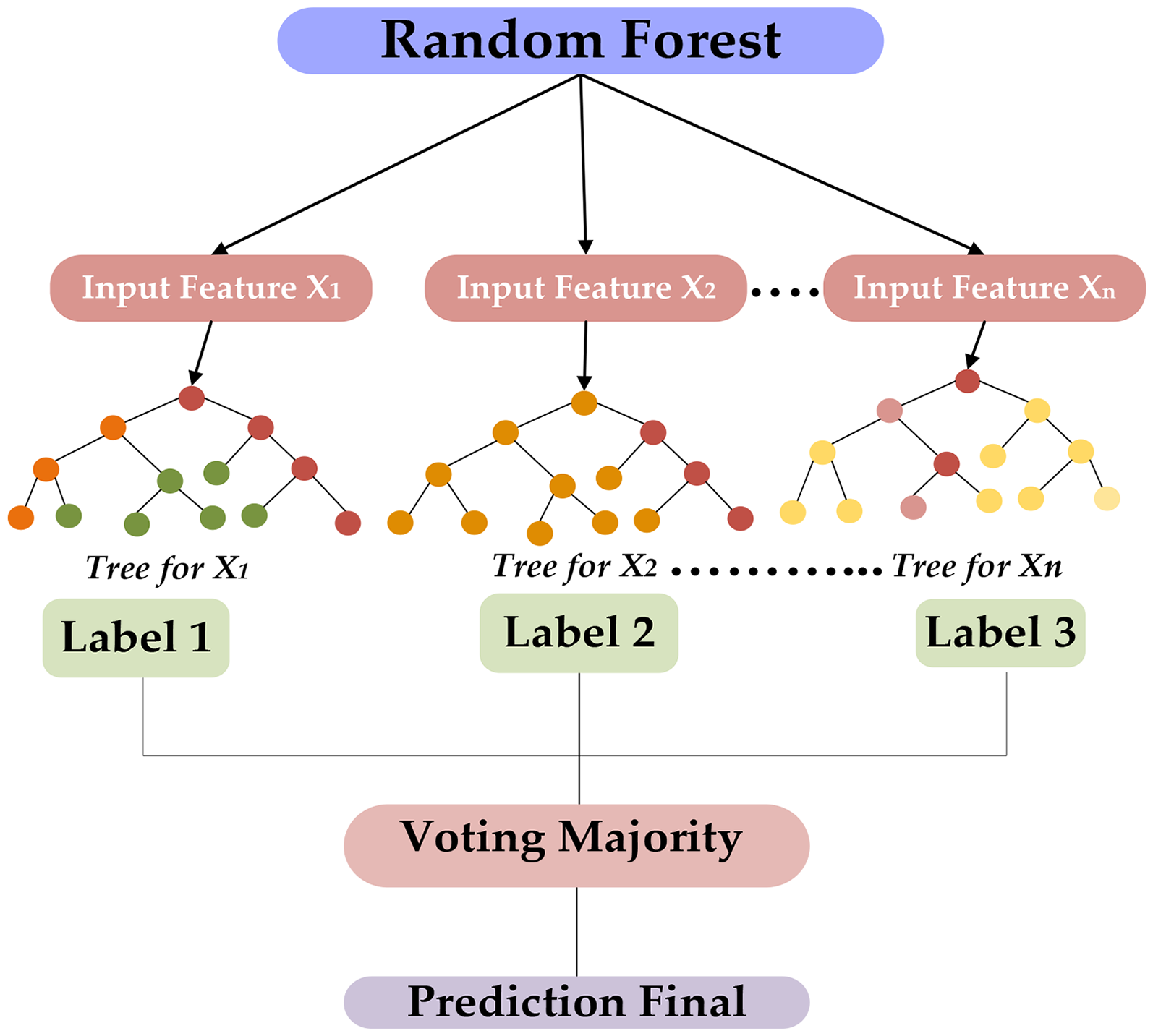
Proposed architecture of random forest for predicted model.

Extra tree

Extra Trees is an ensemble machine-learning algorithm that can effectively handle mutual regression and classification tasks. Like RF, it constructs unique decision trees during training but incorporates random sampling by selecting the split point randomly (see Figure 6). This unpredictability enhances the diversity of the trees in the ensemble, improving the predictive model's flexibility and general capacities while reducing the possibility of overfitting. During forecasting, the results of all the trees are combined, usually by majority vote for classification tasks or average for regression. ⁴³ The ETs algorithm's nonparametric nature, high classification accuracy, and significance of feature evaluation are among its advantages. It efficiently handles a variety of characteristics, that is, raw moments, central moments, and Hahn moments, which are 1-D vector representations of protein structures. Additionally, these vectors capture the positional and spatial information of amino acids by incorporating the raw moments, central moments, and Statistical moments of PRIM and RPRIM. ⁴² The FM, AAPIV, RAAPIV, and their conversions are examples of genomic, proteomic, and computational biology computed data. A primary vector with dimensions of 153 + 2r is formed, with r standing for extra feature-specific dimensions. Every feature vector is used by the ETs model to formulate a FIM, whereas each row represents a different model. Classification into continuous component classes (such as positive or negative) within the FIM is formed by the FOM. The number of decision trees in the ensemble was given by the parameter n_estimators = 100 using the model. To guarantee repeatable results, a fixed random_state = 42 was employed to preserve consistency in data shuffling and tree formation across runs. While the algorithm's consistency was evaluated by forming computations on the training data, the dataset was analyzed during training to recognize basic patterns. Compared to RF, ETs introduced additional randomness by choosing both the features and the splitting thresholds arbitrarily at each node, which helped to reduce model variance and improve generalization. The classifier proven robust predictive performance and contributed to evaluating the discriminative strength and robustness of the extracted proteomic features.

Figure 6.

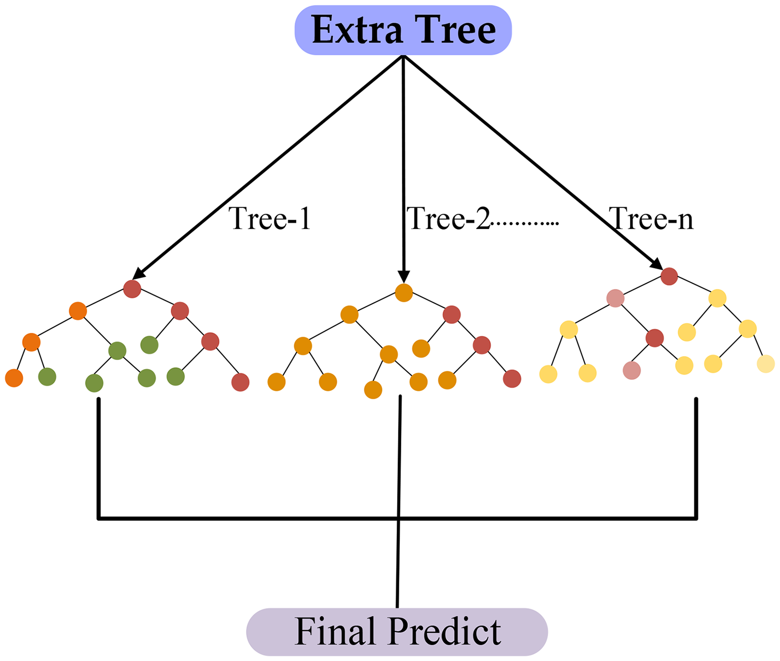
Proposed architecture of extra trees for predicted model.

Convolutional neural network

A 1-D CNN specific for sequences of amino acids is utilized to evaluate 1-D protein patterns. Convolutional layers identify features. Nonetheless, pooling layers reduce dimensionality while preserving significant information. Fully connected (FC) layers perform algorithms, with activation functions to observe nonlinear interactions as depicted in Figure 7. Dropout is applied to avoid overfitting.^60,50 CNN 1-D models are efficient at recognizing the structure of proteins and essential features, making them beneficial in proteomics and biological computation. They improve the identification of protein function and patterns of structure in biological and health research. The CNN model implemented a MaxPooling1D layer to reduce dimensionality and identify the most prominent local features after three convolutional layers with filter sizes of 32, 64, and 128 each employing a kernel size of 3. Overfitting was reduced by applying a dropout layer at a rate of 0.2. The extracted features were fed into a FC dense layer with 128 units, which followed by an output layer with a sigmoid activation function for the binary classification. According to CNN 1-D, the method has various benefits, including outstanding accuracy and the ability to measure variable significance. It evaluates feature extract that consists of raw moments, central moments, and Hahn moments, which signify Protein structures in 1-D vectors and are supported by the FM, APPIV, and RAAPIV. These vectors create a FIM, which is converted into the FOM for classification parameters. This approach is frequently employed in genomics, statistical proteins, and bioinformatics computational for binary classification, defending its ability to handle complex data with maximum accuracy.

Figure 7.

Proposed architecture of CNN 1-D for predicted model.

Multilayer perceptron

A MLP is a kind of feedforward artificial neural network, also known as an ANN, that is, commonly utilized for regression and classification tasks. ⁶¹ Multilayer Perceptron has helped discover diabetes by evaluating protein features determined by proteomic and genomic data. These proteomic features consist of AAC, positional facts, and statistical moments, that is, raw, central, and Hahn moments, all of which provide focal insights into the structure of proteins and the efficient roles of diabetes-related proteins. Multilayer Perceptron computes statistical feature vectors derived from sequences of protein. These vectors commonly contain essential facts, such as the FM, amino acid frequencies, the AAPIV, and the RAAPIV, which encode relative information. ⁴² Furthermore, PRIM and RPRIM moments signify spatial correlations in statistics between amino acids in proteins. Multilayer Perceptron hidden layers convert these features using nonlinear activation functions, such as Relu helpful complex linkages in the facts. For binary classification tasks, the output layer employs a single neuron with a sigmoid activation function (see Figure 8) to compute predict results like diabetic or nondiabetic categories. Multilayer Perceptron algorithms are trained by applying optimization that includes Adam, with hyperparameters such as Adam 0.001 learning rate, batch size is 32, and 100 epochs carefully determined to maximize implementation. These models are extremely effective at mixing various protein features, resulting in accurate classification and discovery of significant identified diagnostics for DM.

Figure 8.

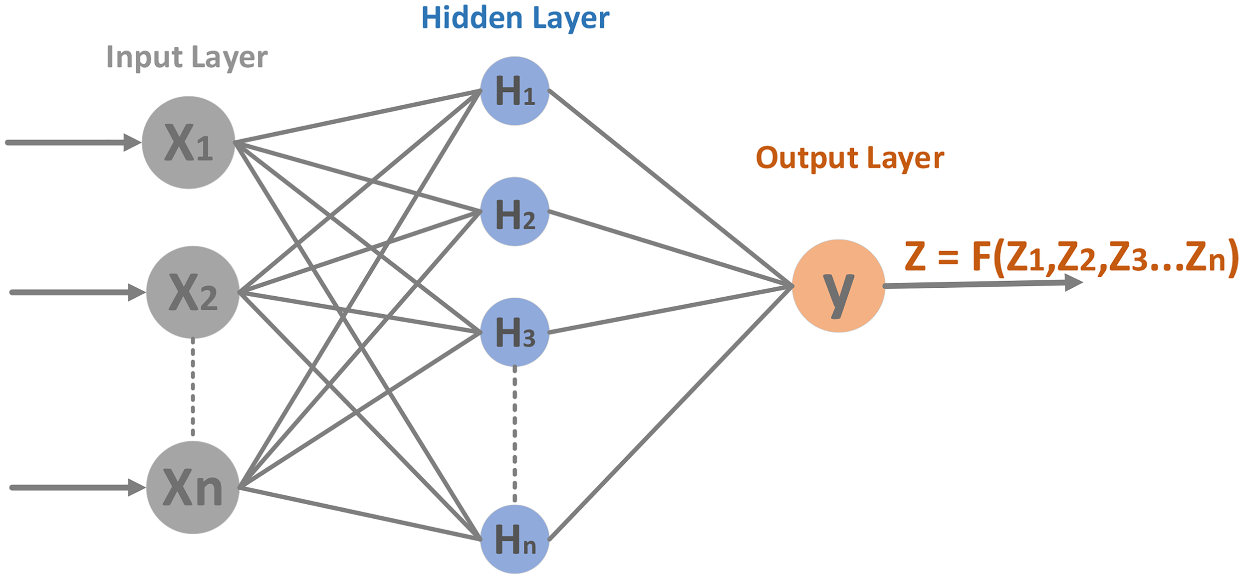
Proposed architecture of MLP for predicted model.

Long short-term memory

Long Short-Term Memory is another kind of RNN (recurrent neural network) that addresses the limitations of typical deep neural networks in finding long-term dependent states in sequential data. Standard RNNs are frequently difficult to train on extended sequences of data due to gradients that vanish or explode. The LSTMs address this issue through their unique structure, which allows them to keep and access data over varied periods, proving particularly effective for sequential tasks such as sequence proteins in computational biology. The LSTM concept is formed a memory cell and three gates of input, forget, and output. These gates control the flow of data, allowing the model to keep only relevant information, modify the memory state with new input, and discard obsolete information.^50,54,62 The input gate specifies what new information should be retained, the gate for forgetting specifies what should be erased from memory, and the gate at the output defines what information to send on to the next stage of time (see Figure 9). This gating function is essential for the LSTM's ability to discover short-term and long-term dependence. LSTM models perform well in managing sequential information with complicated temporal correlations, presenting flexibility and efficiency in identifying and modeling trends throughout time. In training configurations, the model commonly contains extensive output layers and is optimized with parameters such as epochs 100 and size batch of 32.

Figure 9.

Proposed architecture of LSTM for predicted model.

Metrics performance evaluation

The purpose model is computed by different metrics such as accuracy score, specificity, sensitivity, and Matthew's correlation coefficient. The accuracy score reveals the amount of all sorts of samples from both the classes correctly predicted all sorts of samples. For the purposes of quantifying the obvious negatives that can be anticipated from the accuracy of the model specificity has been used. Sensitivity is how well the model can discover the presence of positivity. Even with unbalanced data, since Matthews correlation coefficient (MCC) considers both classes it is a reliable metric. If the model can be able to identify both positive and negative samples, it will produce a reliable MCC score. For every metric considered, ⁶³ the formulas are given:

$$\mathrm{Accuracy}={\displaystyle \frac{TP+TN}{TP+TN+FP+FN}}$$

(18)

$$\mathrm{Specificity}={\displaystyle \frac{TN}{TN+FP}}$$

(19)

$$\mathrm{Senstivity}={\displaystyle \frac{TP}{TP+FN}}$$

(20)

$$\mathrm{MCC}={\displaystyle \frac{TN\times TP-FN\times FP}{\sqrt{(FP+TP)(FN+TP)(FP+TN)(FN+TN)}}}$$

(21)

A True Positive is the protein from the positive class, which is correctly predicted by the predictor. False Negative means that this protein belongs to the positive class but is predicted as negative. On the other hand, False Positive means Negative samples, but the predictor predicts Positive samples. A True Negative represents the negative class samples, which are correctly classified by the predictor.

Algorithms used for the prediction of experiments and results

The performance of the proposed approach is evaluated utilizing some kind of approaches that evaluate and validate its predicted accuracy. Various parameters and measurements are employed to evaluate the efficiency of the classifiers, providing a thorough evaluation of the algorithm's performance.

Validate the prediction outcome on an independent dataset, self-consistency, and 10k-fold cross-validation

Evaluation of prediction using an independent test set

An independent test set is a subgroup of data that is not applied to train predictive algorithms. Instead, it is used just to evaluate the model's performance after training. Using an independent test set provides a precise analysis of the algorithm's generalization capabilities if it performs well on new, unknown data rather than directly overfitting the training set. An independent test set evaluation is the most utilized and significant method to evaluate a prediction model's performance on previously unseen data. In this research, we separated the dataset into two portions: 80% for training and 20% for testing. An algorithm was trained on 80% of the data, and its performance was measured utilizing the remaining 20% as a test set. Table 2 shows the proposed model's accuracy measures for the independent test.

Table 2.

Independent test of the prediction model.

Model	Accuracy	Balance Accuracy	Specificity	Sensitivity	F1-score	Precision	MCC
SVM	84.98	84.08	71.11	97.06	84.43	84.08	0.714
RF	91.46	89.92	82.99	98.85	91.29	90.92	0.836
ET	91.74	91.22	83.72	98.72	91.58	91.22	0.840
CNN	87.03	86.43	95.01	77.85	84.82	93.15	0.746
MLP	81.23	80.07	96.93	63.20	75.81	94.73	0.650
LSTM	83.21	82.28	95.79	68.77	79.22	93.43	0.678

Figure 10 represents the AUC scores of the SVM, RF, ET, CNN 1-D, MLP, and LSTM models. The highest predicted accuracy for DMs using supervised models on the independent tests was 91% (ETs) and 87% (1D-CNN).

Figure 10.

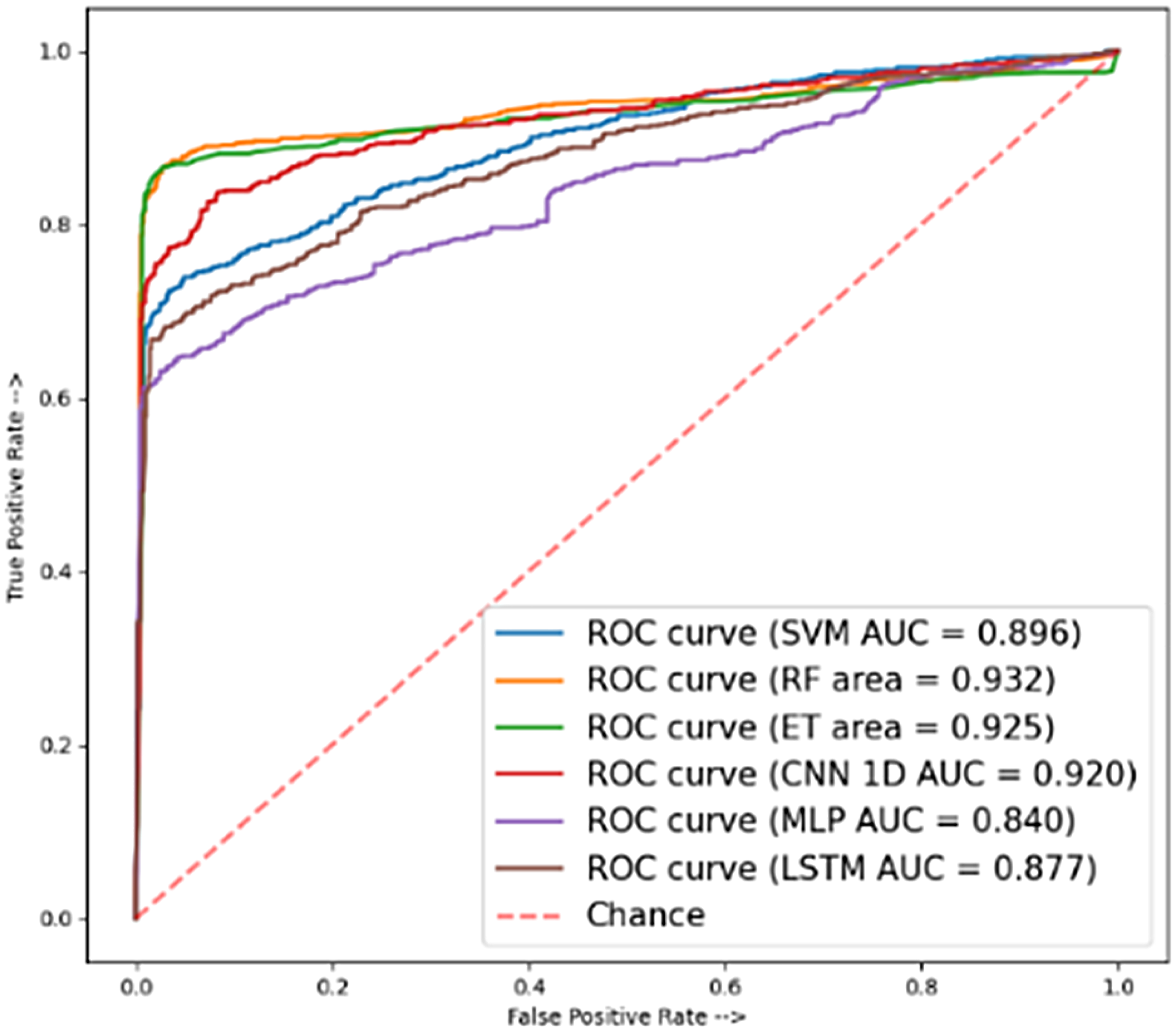
ROC curve of independent test.

Evaluation of prediction using the self-consistency test

A self-consistency test was utilized to validate the model's fitness and evaluate the accuracy of the predictor's training. Before analyzing the model's training effectiveness, feature vectors were generated utilizing both +ve and -ve data from the dataset to validate its performance. A 0.2 split was utilized for the self-consistency test, and all the classifieds from the dataset were tested to validate that the model's data was accurate. Table 3 presents the accuracy measurements achieved from the self-consistency test for each classification algorithm, such as the RF classifier and the final FC layer. The results showed that the most complex representations outperform FC sigmoid layers when utilized with the RF classifier. As a result, the RF classification was chosen for additional research. Although the self-consistency test gives an overview of model performance, it may overlook certain anomalies detectable in independent test sets. Cross-validation is a common recommendation for more comprehensive performance explores curves for SVM, RF, ET, 1D-CNN, MLP, and LSTM models.

Table 3.

Self-consistency of prediction model.

Model	Accuracy	Balance accuracy	Specificity	Sensitivity	F1-score	Precision	MCC
SVM	97.40	97.35	97.59	97.20	97.40	97.59	0.948
RF	92.40	92.41	98.79	86.02	92.37	93.09	0.855
ET	92.01	93.14	84.01	98.97	91.85	91.49	0.846
CNN	94.00	93.95	88.30	99.60	94.36	89.64	0.885
MLP	97.70	97.70	98.17	97.24	97.72	98.21	0.954
LSTM	98.50	98.50	98.01	98.99	98.49	98.00	0.970

Figure 11 represents the AUC scores overall best accuracy of the DM using supervised models on the self-consistency were 0.998 (SVM) and 0.999 (LSTM).

Figure 11.

ROC curve of self-consistency.

Evaluation of prediction using 10k-fold cross validation

Cross-validation is carried out via a subsampling test that partitions the dataset into k-folds. In this test, just one-fold is used for testing, with the remaining k-1 folds used to train the model. Every fold is tested exactly once during the k repetitions of this technique. In this test, the 10k-fold subsampling test is employed. The main drawback of the subsampling test is that it returns inconsistent findings for the same predictor and dataset depending on the folds used. The samples are chosen at random each time to create the folds, hence, the results of a subsampling test do not differ for a particular dataset. The represented Table 4 each predictor model with the features selected obtained Accuracy metrics of 89.30, Balance Accuracy values of 89.30, Specificity values of 88.20, Sensitivity values of 90.40, F1-Score value of 89.15, and MCC values of 0.786 in the ET model, and Accuracy metrics of 87.60, Balance Accuracy values of 87.58, Specificity values of 87.64, Sensitivity values of 87.52, F1-Score value of 87.74, and MCC values of 0.753 in the MLP model for genomic protein feature. In terms of achievement, the model incorporating all features outperformed the one using selected features. On the other hand, Figure 11 represents the AUC scores, overall the best accuracy of 10k-fold cross validation was 0.941 and 0.958, with the ET and MLP performing better than others.

Table 4.

10k-Fold cross validation of prediction model

Model	Accuracy	Balance accuracy	Specificity	Sensitivity	F1-score	Precision	MCC
SVM	86.00	86.00	89.00	83.00	85.49	88.47	0.786
RF	89.30	89.30	90.40	88.20	89.15	90.32	0.786
ET	88.60	88.60	90.40	86.80	88.34	90.18	0.773
CNN	82.00	81.97	79.40	84.57	82.64	81.15	0.643
MLP	87.60	87.58	87.64	87.52	87.74	88.15	0.753
LSTM	56.30	56.15	37.42	74.89	62.30	54.91	0.146

Predict comparison of DM

To contribute to exploring the effect methodology, we precisely derived a UniProt/Swiss-Prot and NCBI database containing DM proteins. Researchers used sophisticated feature extraction techniques to develop vectors of feature-specific size for each protein, which significantly improved subsequent procedures, that is, classifying model train and evaluation. We evaluated the efficiency of various algorithms of supervised learning, that is, ML and DL algorithms to predict protein functions utilizing different protein amino acid features. The models evaluated include SVM, RF, 1-D CNN, MLP, and LSTM, with comparisons performed across various protein features. In the independent test, the ET and 1D-CNN models achieved an accuracy of 0.91 and 0.87, SVM and LSTM achieved the accuracies of a self-consistency accuracy of 0.97 and 0.98, and 10-fold cross-validation accuracy of 0.89 and 0.87 using RF and MLP. Among the genomics features, the AAC outperformed all the others. Additional analysis is possibly essential to better the performance of these models across various features. On the other hand, Figure 10 proved the ROC curves for each algorithm of an independent test, showing that the CNN achieved an AUC of 0.92; RF slightly outperformed it with an AUC of 0.93. Figure 12 also proves that achieved AUC of 0.99 in RF and 0.99 in LSTM of ROC for the self-consistency test, in which the RF and MLP models with the genomic features achieved a 10-fold cross-validation AUC of 0.94 and 0.95.

Figure 12.

ROC curve of 10k-fold cross validation.

In this section, visualizing decision boundaries provides an intuitive way to identify how different classification algorithms separate data points in various classes. With real training and testing by plotting the approximate areas of each model, any alignment can inspect or monitor between the bound and the underlying distribution. According to visualization and accuracy evaluations shown in Figure 13, SVC and RF are tied for the best performance on the Decision Boundary Visualization (0.91). Overall, ML methods (SVC, RF, ETs) perform better than DL methods (MLP, CNN, LSTM) models in various actual tasks, while the results vary by dataset.^43,41 When analyzing complex biological datasets such as DM genomics expression, the t-SNE may not yield clear splits because it transforms high-dimensional data (153 feature genomics feature) into a 2D space.

Figure 13.

Result of decision boundary visualization.

Discussion

In this section, we proposed a supervised learning framework utilizing a variety of model-based classification, such as both DL and standard ML approaches, to computationally identify diabetes-associated proteins. A set of developed features, including statistical vector encodings, AAPIV, RAAPIV, RPRIM, and PRIM, ⁴³ have been extracted from protein sequences retrieved from the NCBI^36,37 and UniProt ³⁸ databases to improve the models’ predictive performance and biological interpretability. In order to identify sequence-level structures in proteomics, these features were implemented to preserve both positional and compositional characteristics. All evaluation techniques, such as independent test, self-consistency, and k-fold cross-validation, showed consistently better performance from the ensemble-based classifiers, specifically RF and ETs, as shown Table 2. These results are in line with prior studies revealing that ensemble approaches, which combine predictions from several weak learners to enhance generalization and stability, are particularly efficient when utilizing biological data. As demonstrated by previous studies in protein structure-function prediction, the reliability and validity of RF and ET in this experiment further validate the significance of ensemble learning for complex, high-dimensional proteomic classification tasks. In contrast, SVMs produced inconsistent results across validation methods. This variation is consistent with previous studies that identified the limitations of the SVM when dealing with nonlinearly separable data or datasets with class imbalance both of which are common in biological sequence data. The observed performance drop under independent validation suggests that SVM may not generalize as well in scenarios where the distribution of data is nonuniform or sparse, a limitation observed in previous applications involving similar datasets.

In sequence recognition of patterns DL algorithms such as CNN-1D, MLP, and LSTM demonstrated respectable abilities, especially when evaluated for self-consistency. On the other hand, their performance varied more widely across validation types, probably due to the difficulties associated with training sophisticated algorithms on moderately large datasets. This observation is consistent with previous research findings, which have shown that DL techniques require large-scale datasets or more complex training strategies that include transfer learning or pretraining on larger protein databases, to achieve their full potential. Importantly, the proposed forecasting framework's success was due not only to the classifiers but also to the effective integration of biologically relevant representations of features. The use of domain-informed developed features enhanced model learning and comprehensibility which is a strategy increasingly utilized in computational biology to balance predictive accuracy with biological insight. The findings of this study lend further support to hybrid methodologies that handle protein classification challenges by combining structured feature extraction with effective ML algorithms. Overall, these findings highlight the importance of ensemble learning in biological sequence analysis and the beneficial effects of interpretable feature extraction in proteome-based prediction of diseases. The proposed strategy provides a viable and scalable solution for high-throughput protein identification in DM, providing improved methodology and tangible benefits to the field of computational proteomics.

Conclusion and future

In this article, we propose an experimental method for the prediction of proteins that relate to DM. The method we employed includes comprehensive, statistically rigorous analysis that includes the implementation of various evaluation methodologies to ensure the validity of our findings. We utilized the evaluation of predication using independent testing, 10k-fold cross-validation, and self-consistency to validate the accuracy of DM protein forecasts. The supervised learning methodologies have proven great ability in developing a classifier for DM protein. By leveraging the power of deep neural networks, researchers can extract features from protein or peptide sequences and predict their DM function with high accuracy. We developed a classifier that accurately identifies DM-related proteins by assembling a dataset of annotated protein sequences, training ML models on the UniProt/Swiss-Prot and NCBI dataset and evaluating its performance on test sets. We extracted the feature of protein sequence using Python. The Python algorithms for ML were used to identify feature descriptors and build a model to help in protein sequence analysis and prediction. The Sequence Proteins are transformed into a numerical form, known as the extraction feature of encoding in genomic proteomics. The analysis results indicate that the proposed classifier outperforms these methods, exhibiting superior performance in identifying DM peptide sequences using prediction using numerical vectors. These encoded sequences were analyzed using the proposed models, that is, SVM, RF, ET, CNN, MLP, and LSTM algorithms. The self-consistency validation yielded an accuracy of 98.50%, specificity of 98.01%, sensitivity of 98.99%, and a MCC of 0.970. In the 10-fold cross-validation, we obtained an accuracy of 88.60%, a specificity of 90.40%, a sensitivity of 86.80%, and a MCC of 0.773%. Finally, the outcome of the independent test yielded an accuracy of 91.74%, specificity of 83.72%, sensitivity of 98.72%, and a MCC of 0.840. We have conducted these analyses using a variety of computational methods, that is, AI encompasses ML, of which DL, a subfield of ML, includes techniques such as Support Vector, RF, ETs, 1D-CNN, MLP, and LSTM. The RF model performed extremely well, exceeding other techniques in the majority of evaluations. The proposed prediction model accurately identifies diabetes-related proteins, with the potential to identify novel therapeutic targets and diagnostic markers. Future research could investigate the effort of novel protein sequences to improve accuracy in forecasting and comprehension of DM.