Sage Journals: Discover world-class research

Abstract

Background

The construction of a model to estimate patients’ status in early-stage diabetic kidney disease (ES-DKD) is needed. Thus, the risk factors playing a role in the disease diagnosis can be determined when routine examination outcomes are collected.

Objective

Routine examination outcomes can also be used to predict patients’ ES-DKD. A first-stage study is conducted on how successful conventional statistical models (CSMs) perform when sample sizes are small when compared to machine learning methods (MLMs).

Methods

A total of 268 observations were collected from two tertiary hospitals in Lanzhou with demographic information, basic medical history, and routine laboratory tests such as blood routine, common biochemical tests, and urine routine. Then, conventional statistical methods and MLMs are applied to establish models separately to determine optimal prediction models. In addition, machine learning has also been applied to establish fused models to explore new modeling methods.

Results

The validation set can better represent the actual performance of the models in clinical practice. Therefore, the comparisons are made based on the predictive performance of the two methods using the validation set. Ultimately, it was concluded that the ensemble model outperforms in terms of performance metrics. The CSMs perform poorly in terms of area under curve values. Compared to various MLMs, the performance of others is not inferior.

Conclusion

This article establishes multiple ES-DKD prediction models using CSMs and MLMs. New ideas and methods for the diagnosis, treatment, and prevention of ES-DKD in clinical practice are presented. This article also compares two modeling methods. A comprehensive model was established, which has excellent predictive and generalization ability and stability. Therefore, the integration of the advantages of MLMs based on CSMs is a very fruitful attempt. Fused models have a high chance of being the main research direction for future research to develop better models.

Keywords

Diabetic kidney disease type 2 diabetes mellitus mathematical model prediction

Introduction

The 10th edition report of the International Diabetes Federation (IDF) estimates that one out of 10 people is diagnosed with diabetes, and the number of patients increases constantly.¹ Diabetic kidney disease (DKD) is a common complication in diabetic patients. For example, the incidence of DKD in diabetic patients accounts for about 20%–40% of the population in China.² DKD has become the main cause of chronic kidney disease (CKD) and has resulted in renal disease even in the end stages.^3,4 A renal biopsy, as a gold standard to diagnose the DKD, is invasive.^5,6 However, its administration is poorly accepted by patients. Currently, urinary albumin-to-creatinine ratio (UACR), urinary albumin excess rate (UAER), and estimated glomerular filtration rate (eGFR) are widely administered in the clinical diagnosis of DKD.⁷ Nevertheless, in the early stages of diseases, these indicators may not fluctuate significantly and provide detailed information, and some indicators are not reported in routine examinations, which can impair the patient's condition in the long run. If DKD is not treated timely, the symptoms get worse, and the stage of uremia and even fatal consequences are inevitable. Hence, finding easy and reliable ways to diagnose based on routine examination scores and not highly depending on using invasive methods is practically significant for patients who have potential DKD at early stages.

To find data-oriented methods, many researchers suggested mathematical models to predict DKD at an early stage as a diagnosis tool, so that the prediction and prognosis of diseases can be easily conducted. Hence, ambiguous diagnostic guidelines and invasive methods to diagnose DKD at an early stage could affect the patients less. To construct mathematical-based modeling in general, two sets of models, namely, conventional statistical models (CSMs) and machine learning methods (MLMs) can be used. Each group is equipped with its advantages and disadvantages. Although much research applies those two sets of modeling tools separately to determine better outcomes, a limited study has been conducted to compare them.

To compare those two sets of tools, the early predictive model for diabetic nephropathy was established, and the two methods were compared under the same conditions such as small sample size, the same data set, the same output variable, and the same grouping method to investigate how the CSMs and MLMs perform in the small sample sizes.

Methodology

The objective of the research

The research is a case-control study that had 179 cases in the 940th Hospital of the Joint Logistics Support Force of the Chinese People's Liberation Army (Hospital A) between 2018 and 2022 as the training set, and 89 cases in the First Hospital of Lanzhou University (Hospital B) from 2018 to 2022 as the test set. The two data sets are independent. Using EpiData software, under the same template and rules, patients’ data were collected randomly.

First of all, all patients have been clinically diagnosed with diabetes mellitus type 2 (T2DM). Secondly, patients in the early-stage diabetic kidney disease (ES-DKD) group were also clinically diagnosed as early diabetes nephropathy patients based on T2DM. In addition, DKD patients are clinically diagnosed according to diagnostic guidelines, patient history, B-ultrasound, whether there is diabetes retinopathy, puncture biopsy, and other methods.

According to the internationally recognized critical score of the DKD, the guideline for improving global outcomes (KDIGO) has been published for the reliability of the data.⁸ The patients in the T2DM group (non-ES-DKD group) and the ES-DKD group were screened through the chronic kidney disease epidemiology collaboration equation (CKD-EPI).^9,10 The diagnosis of DKD in the early stage, which is mild symptoms, and the changes in diagnostic indicators not being obvious, will be conducted based on data analysis. The “low risk” stage is defined as the ES-DKD score, which is the EGFR ≥ 60 mL/min/1.73 m². Due to occasional normal and elevated eGFR levels of 120 in patients with ES-DKD, this study only limited the lower limit of eGFR in the ES-DKD group and did not limit the upper limit.

DKD is a microvascular complication of diabetes, and diabetes retinopathy is also a microvascular complication. To exclude the interference of diabetes retinopathy, the non-ES-DKD group excluded diabetes retinopathy. Patients with kidney cancer and kidney tumors who suffer from severe kidney damage may have biased results, so both groups excluded such patients. Therefore, the following inclusion and exclusion criteria have been formulated.

Figure 1 defines both inclusion and exclusion criteria. The non-ES-DKD group includes patients who were clinically diagnosed with T2DM and never had diabetic microangiopathy such as ES-DKD, or diabetic retinopathy. Their eGFR values were 120–90 mL/min/1.73 m². Patients without renal tumors or renal cancer were included. The ES-DKD group contains patients with clinically diagnosed type 2 diabetic nephropathy with eGFR ≥ 60 mL/min/1.73 m². Patients without renal tumors or renal cancer were also included. Also, patients were excluded with missing data in the training and validation sets. The final training sets consisted of 75 non-ES-DKD group patients and 89 ES-DKD group patients, respectively, while the validation set consisted of 37 non-ES-DKD group patients and 49 ES-DKD group patients. The data were collected with all signed and informed consent by the patient upon admission. The ethics committees of both hospitals approved the content of the study.

Figure 1.

Data entry and discharge process.

Methods

Both deduplication and denoising processes are conducted on datasets. The patients were excluded from the experiment. The qualitative attributes of the two datasets were coded. Finally, CSMs and MLMs were implemented to construct prediction models and were compared. The training sets were employed to construct the prediction models, and the validation sets were implemented to verify the results of the predictions.

Indicators

Table 1 presents quantitative data that includes age and laboratory indicators such as blood routine, biochemistry, renal function, HbA1c, and so on. Table 2 summarizes the qualitative attributes which are gender, hypertension history, other related history variables for kidney diseases, insulin utilization history, glycemic control, heredity, smoking, drinking, the history of T2DM (5 years as the boundary), urine pH, proteinuria, the history of T2DM (10 years as the boundary), and basic diseases. Other kidney diseases refer to kidney diseases other than diabetic kidney disease such as renal calculi, renal cysts, hydronephrosis, and so on. Urine pH is assigned to 6 as the cut-off point, and if < 6 the acidic stage is considered. Proteinuria is the presence of “+” as the cut-off point, namely, classified as positive or negative. Basic diseases refer to the presence of other diseases other than diabetes and its complications. Heredity refers to whether the family has a genetic history of type 2 diabetes. The onset time of T2DM is determined by the time from the patient's first diagnosis to the time of data collection. The history of T2DM, which is 5 years of illness, is accepted as the boundary since patients with a diabetes history of > 5 years may develop microvascular lesions. In the article, it is set since it will be used as an interference indicator of whether MLMs can eliminate similar interference. The history of T2DM, which is 10 years of illness, is accepted as the boundary since patients with a diabetes history of > 10 years may be the main cause of DKD.¹¹

Table 1.

The results of the single-factor analysis are based on quantitative data.

Project titles	Non-ES-DKD	ES-DKD	p-value*
Project titles	Median (IQR)/mean ± SD	Median (IQR)/mean ± SD	p-value*
Age, years	55.3700 ± 11.3360	59.0100 ± 11.8490	0.0474
Systolic blood pressure (SBP), mmHg	135.2100 ± 17.7320	135.0000 (125.0000–150.5000)	0.1625
Diastolic blood pressure (DBP), mmHg	80.7700 ± 10.8310	79.0000 (74.0000–87.5000)	0.9947
BMI, kg/m²	25.1137 ± 3.0596	24.9276 ± 3.4669	0.7185
White blood cell count (WBC), 10⁹/L	5.5600 (4.9200–6.7600)	5.5400 (4.8000–7.0650)	0.8884
Red blood cell count (RBC), 10¹²/L	4.8468 ± 0.5661	4.7703 ± 0.6131	0.4112
Hemoglobin (HGB), g/L	148.9600 ± 16.3669	144.8876 ± 18.9031	0.1461
Hematocrit (HCT), %	43.9387 ± 4.6055	43.0539 ± 5.3697	0.2639
Mean corpuscular volume (MCV), fL	90.9267 ± 5.1201	90.4112 ± 4.8497	0.5096
Mean hemoglobin content of red blood cells (MCH)pg	30.9000 (30.0000–32.1000)	30.4180 ± 1.8497	0.0601
Mean corpuscular hemoglobin concentration (MCHC), g/L	339.1333 ± 9.6034	336.3483 ± 9.1342	0.0592
Platelet (PLT), 10⁹/L	179.7600 ± 49.4729	186.6742 ± 67.6254	0.4518
Percentage of lymphocytes (L%), %	32.9987 ± 11.0246	30.9607 ± 8.4647	0.1929
Percentage of monocytes (M%), %	6.2000 (5.4000–7.1000)	6.9034 ± 1.6553	0.0557
Percentage of neutrophils (N%), %	57.5907 ± 11.3826	59.1247 ± 9.3108	0.3439
Percentage of eosinophils (EO%), %	1.9000 (1.1000–2.9000)	1.7000 (1.2000–3.1000)	0.7214
Basophil percentage (BASO%), %	0.3000 (0.2000–0.5000)	0.4000 (0.2000–0.5500)	0.0852
Lymphocyte count (L), 10⁹/L	1.8944 ± 0.7155	1.7500 (1.4400–2.1950)	0.3835
Monocyte count (M), 10⁹/L	0.3500 (0.2900–0.4300)	0.4000 (0.3000–0.4850)	0.0803
Neutrophil count (N), 10⁹/L	3.2100 (2.4900–3.8700)	3.4400 (2.6000–4.1250)	0.4139
Eosinophil count (EO), 10⁹/L	0.1000 (0.0500–0.2000)	0.1000 (0.0800–0.2000)	0.4238
Basophil count (BASO), 10⁹/L	0.0100 (0.0000–0.0200)	0.0100 (0.0000–0.0300)	0.3442
Coefficient of variation of RBC distribution width (RDW-CV), %	13.0000 (12.5000–13.6000)	13.3000 (12.9000–13.8000)	0.0049
Platelet distribution width (PDW), %	16.2000 (13.8000–16.7000)	15.9000 (13.7000–16.7000)	0.9158
Mean platelet volume (MPV), fL	11.2613 ± 1.1934	11.7157 ± 1.2083	0.0170
The standard deviation of red blood cell distribution width (RDW-SD), fL	42.7000 (40.8000–44.9000)	43.7000 (41.6500–45.7500)	0.0553
Platelet crit (PCT), %	0.2011 ± 0.0539	0.2162 ± 0.0750	0.1370
Large platelet ratio (PLCR), %	36.0573 ± 9.0765	39.3000 (31.8500–45.2000)	0.0503
Lactate dehydrogenase (LDH), IU/L	161.0000 (136.0000–198.0000)	168.0000 (144.0000–191.0000)	0.4923
α-hydroxybutyrate dehydrogenase (α-HBDH), IU/L	139.0000 (121.0000–167.0000)	143.0000 (120.5000–165.5000)	0.8832
Creatine kinase (CK), IU/L	73.0000 (54.0000–96.0000)	84.0000 (60.0000–115.5000)	0.2097
Creatine kinase isoenzyme (CK-MB), IU/L	9.0000 (7.0000–12.0000)	10.0000 (7.0000–12.5000)	0.3044
Aspartate aminotransferase (AST), IU/L	22.0000 (17.0000–31.0000)	20.0000 (16.0000–27.0000)	0.0684
Alanine aminotransferase (ALT), IU/L	24.0000 (16.0000–43.0000)	19.0000 (15.0000–30.0000)	0.0141
AST/ALT	0.9100 (0.7400–1.1600)	0.9900 (0.7750–1.3050)	0.0779
Total protein (TP), g/L	68.1253 ± 6.6987	67.0090 ± 7.8665	0.3344
Albumin (ALB), g/L	43.0787 ± 3.2766	41.7000 (38.9500–44.1500)	0.0081
Globulin (G), g/L	25.0507 ± 4.5368	25.6000(22.6000–28.3500)	0.3693
A/G	1.8000 (1.5000–1.9000)	1.6213 ± 0.3553	0.0090
Total bilirubin (TBIL), μmol/L	15.5000 (12.0000–19.2000)	13.8000 (9.9500–19.4000)	0.1142
Direct bilirubin (DBIL), μmol/L	2.9000 (2.3000–3.5000)	2.7000 (2.1000–3.8500)	0.2890
Indirect bilirubin (IBIL), μmol/L	12.5000 (9.7000–15.3000)	10.8000 (7.9000–15.3500)	0.1009
Alkaline phosphatase (ALP), IU/L	88.0000 (71.0000–106.0000)	93.0000 (75.0000–111.0000)	0.2282
γ-glutamyltransferase (GGT), IU/L	32.8000 (21.9000–54.2000)	28.5000 (17.9500–51.2000)	0.3799
α-L-fucosidase (AFU), U/L	17.0000 (15.0000–21.0000)	19.0000 (15.0000–21.0000)	0.3010
Calcium (Ca), mmol/L	2.2568 ± 0.1293	2.2400 (2.1500–2.3000)	0.0429
Phosphorus (P), mmol/L	1.1865 ± 0.1805	1.1611 ± 0.2005	0.3988
Potassium (K), mmol/L	3.9925 ± 0.3165	3.9600 (3.7400–4.1850)	0.7177
Sodium (Na), mmol/L	139.0000 (138.0000–140.0000)	139.0000 (138.0000–141.0000)	0.4151
Chlorine (Cl), mmol/L	105.0000 (103.0000–107.0000)	105.0000 (103.0000–107.0000)	0.5494
Carbon dioxide (CO₂), mmol/L	27.2480 ± 2.7559	25.8231 ± 3.0594	0.0022
Anion gap (AG), mmol/L	10.8027 ± 2.3269	12.8303 ± 2.7958	<0.0001
Glucose (GLU), mmol/L	8.0600 (6.6600–9.8200)	8.8000 (6.7050–11.9750)	0.2050
Osmolality (OSM), mOSM/L	299.4933 ± 4.6423	301.0000 (298.0000–305.0000)	0.0201
Triglyceride (TG), mmol/L	1.4500 (1.0400–2.2400)	1.5600 (1.0750–2.3150)	0.9119
Total cholesterol (TC), mmol/L	4.3243 ± 1.0839	4.0900 (3.4900–4.8950)	0.6147
High density lipoprotein cholesterol (HDL), mmol/L	0.9900 (0.8700–1.0800)	0.9500 (0.8050–1.1900)	0.6908
Low density lipoprotein cholesterol (LDL), mmol/L	2.6492 ± 0.7461	2.4600 (2.1450–3.0950)	0.5837
Total bile acid (TBA), μmol/L	3.5000 (1.9000–5.5000)	4.0000 (2.9500–7.1500)	0.0358
Urea, mmol/L	4.9840 ± 1.1562	5.6457 ± 1.5777	0.0023
Creatinine (CRE), μmol/L	63.6933 ± 10.1302	70.3225 ± 17.3961	0.0028
Blood urea/Creatinine (BUN/CREA)	75.0000 (67.0000–95.0000)	81.0000 (67.0000–94.5000)	0.4871
Uric acid (UA), μmol/L	314.0000 ± 72.5715	332.8427 ± 77.4862	0.1123
Estimated glomerular filtration rate (eGFR), mL/min/l.73 m²	102.8264 ± 6.7018	96.5967 (83.0558–104.0291)	<0.0001
Urine specific gravity (SG)	1.0200 (1.0200–1.0250)	1.0200 (1.0150–1.0250)	0.1609
Homocysteine (HYC), μmol/L	13.0400 (10.2900–16.6300)	13.1100 (10.7600–15.8850)	0.9671
HbA1c,%	7.3000 (6.3000–9.6000)	8.6035 ± 1.8722	0.0369
Cholinesterase (ChE), U/L	8300.5300 ± 1890.7960	8180.8900 ± 1697.7100	0.6701

* p < 0.05 indicates a statistically significant difference between the non-ES-DKD and the ES-DKD groups. p ≥ 0.05 indicates that there is no statistically significant difference between the non-ES-DKD and the ES-DKD groups.

Table 2.

The results of the single-factor analysis are based on qualitative data.

Project titles	Total (n = 164)	Non-ES-DKD (n = 75)	ES-DKD (n = 89)	p-value*
Project titles	Number (%)	Number (%)	Number (%)	p-value*
Gender				0.7681
Male	114 (69.5%)	53 (70.7%)	61 (68.5%)
Female	50 (30.5%)	22 (29.3%)	28 (31.5%)
Hypertension				< 0.0001
Yes	97 (59.1%)	31 (41.3%)	66 (74.2%)
No	67 (40.9%)	44 (58.7%)	23 (25.8%)
Other kidney diseases				< 0.0001
Yes	47 (28.7%)	10 (13.3%)	37 (41.6%)
No	117 (71.3%)	65 (86.7%)	52 (58.4%)
Using insulin				< 0.0001
Yes	64 (39%)	17 (22.7%)	47 (52.8%)
No	100 (61%)	58 (77.3%)	42 (47.2%)
Glycemic control				< 0.0001
Well	55 (33.5%)	37 (49.3%)	18 (20.2%)
Unsatisfactory	109 (66.5%)	38 (50.7%)	71 (79.8%)
Heredity				0.0096
Yes	42 (25.6%)	12 (16%)	30 (33.7%)
No	122 (74.4%)	63 (84%)	59 (66.3%)
Smoking				0.0976
Yes	50 (30.5%)	18 (24%)	32 (36%)
No	114 (69.5%)	57 (76%)	57 (64%)
Drinking				0.3093
Yes	48 (29.3%)	19 (25.3%)	29 (32.6%)
No	116 (70.7%)	56 (74.7%)	60 (67.4%)
Time of T2DM (5 years as the boundary)				< 0.0001
≤ 5 years	82 (50%)	54 (72%)	28 (31.5%)
> 5 years	82 (50%)	21 (28%)	61 (68.5%)
Urine pH				0.6186
≥ 6	136 (82.9%)	61 (81.3%)	75 (84.3%)
< 6	28 (17.1%)	14 (18.7%)	14 (15.7%)
Proteinuria				< 0.0001
Negative	107 (65.2%)	75 (100%)	32 (36%)
Positive	57 (34.8%)	0 (0%)	57 (64%)
Time of the T2DM (10 years as the boundary)				< 0.0001
< 10 years	107 (65.2%)	67 (89.3%)	40 (44.9%)
≥ 10 years	57 (34.8%)	8 (10.7%)	49 (55.1%)
Basic disease				0.4626
Yes	161 (98.2%)	73 (97.3%)	88 (98.9%)
No	3 (1.8%)	2 (2.7%)	1 (1.1%)

T2DM: diabetes mellitus type 2; ES-DKD: early-stage diabetic kidney disease.

* p < 0.05 indicates a statistically significant difference between the non-ES-DKD and the ES-DKD groups. p ≥ 0.05 indicates no statistical significance between the non-ES-DKD and the ES-DKD groups.

Modeling based on conventional statistical methods

SPSS 21.0 (IBM, USA), R 4.3.2 (R Foundation for Statistical Computing, Austria), and GraphPad Prism 8.2.1 (GraphPad Software, USA), were utilized to construct CSMs. First, univariate analysis was performed. The dataset's normality assumption was conducted by running a nonparametric Kolmogorov-Smirnov test. Indicators conform to normality assumption and the homogeneity of variance test was conducted to run the one-way analysis of variance (ANOVA). If the normality assumption was not violated and the variances were equal, the independent sample t-test was used. If the Normalality assumption was verified and the variances were not equal, the Welch's t-test was conducted. If the normality assumption was not validated, a non-parametric test called the Mann-Whitney U-test was implemented. Also, the qualitative data were tested by the chi-square (χ²) test.

Secondly, the indicators found statistically significant, (p < 0.05), in univariate analysis were screened whether they could be used as independent variables by the LASSO regression model, stepwise regression model, the selection of the optimal subset, and other methods, respectively.

The logistic regression model is selected since it fits into the purpose of the experimentation. The statistically chosen independent attributes were employed in the logistic regression model that was also utilized as the prediction model. Then, the receiver operating characteristic (ROC) curve of the prediction model was drawn, and the area under curve (AUC) of the training set and the test set were computed and compared, respectively.

Finally, R software was implemented to construct the Nomogram, calibration curve, and decision curve analysis (DCA).

The logistic regression model is given by the following equation:

f (x) = \ln (\frac{P}{(1 - P)}) = β_{0} + β_{1} X_{1} + β_{2} X_{2} + \dots + β_{m} X_{m}

(1)

The modified form of the logistic regression model is attained by the following equation:

f (x) = P = \frac{e^{(β_{0} + β_{1} X_{1} + β_{2} X_{2} + \dots + β_{m} X_{m})}}{1 + e^{(β_{0} + β_{1} X_{1} + β_{2} X_{2} + \dots + β_{m} X_{m})}}

(2)

Modeling based on machine learning methods

Python 3.10.13 (Python Software Foundation, USA) was implemented to crunch the data to construct the prediction model based on MLMs.

First, the data was standardized by subtracting the mean from each observation value and dividing by the standard deviation. Each feature has a mean of 0 and a standard deviation of 1. Equation (3) presents the process.

X_{standardized} = \frac{X - μ}{σ}

(3)where X, μ, and σ denote the data, mean, and standard deviation of each feature, respectively.

Standardization transforms the data into a standard normal distribution. Thus, the prediction model is not affected by the different measurement units of the attributes and can extract the relationship between different features.

Next, feature screening is performed. Feature selection is an important technique to reduce the dimensionality of a dataset and improve model performance. The random forest (RF) algorithm is implemented to screen significant attributes to reduce the effect of the high dimensionality problem in the data set. We chose RF for feature selection primarily due to its robustness and interpretability in estimating feature importance. Specifically, RF provides a natural ranking of features by evaluating the decrease in node impurity or the increase in model error when a feature is permuted.¹² These importance scores offer a practical and effective way to identify relevant features without requiring strong assumptions about data distribution or linearity. Moreover, it does not require additional hyperparameter tuning specifically for feature selection, making it more straightforward and stable in practice. RF-based feature selection has been widely adopted across various domains. Díaz-Uriarte and Alvarez de Andrés¹³ demonstrated its effectiveness in gene selection for bioinformatics applications, highlighting its robustness in handling noisy and high-dimensional data. Genuer et al.¹⁴ provided a comprehensive analysis of its theoretical underpinnings and practical utility in variable selection, especially in high-dimensional settings. Furthermore, Kursa and Rudnicki¹⁵ introduced the Boruta algorithm, an extension of RF, to perform all-relevant feature selection with improved stability. These studies collectively support the suitability of RF as a reliable and interpretable tool for feature selection in complex learning tasks.

Also, several datasets in implementations have a problem of imbalanced classes, where some categories have far more observations than others. The performance of the constructed model can be negatively affected by imbalanced assessment when classification problems are under consideration. To resolve the issue, researchers suggested a variety of resampling methodologies to enhance the class distribution of data sets. For example, the SMOTEENN and SMOTETomek algorithms will be utilized to mitigate the imbalanced category problem in the article and effective syntheses from the data sets will be achieved.

The SMOTEENN methodology combines oversampling and undersampling methods. The class imbalance issue was eliminated by the Synthetic Minority Over-sampling Technique (SMOTE) to synthesize new samples and edited nearest neighbors (ENNs) to clean overlapping parts of samples. The SMOTE is based on analyzing the minor samples and synthesizing new minor samples. Then, the ENN is conducted to get rid of samples that may have been mislabeled.

SMOTETomek is another methodology that is used for offsetting imbalanced data categories, which combines SMOTE and Tomek links. Tomek links are a pair of nearest-neighbor samples, but they belong to distinct classes. The category boundaries can be made clearer by removing one or both samples from such a sample pair. When the SMOTE and Tomek links are combined, the classification performance is enhanced by first utilizing the SMOTE methodology to increase the minority class samples and then employing Tomek links to eliminate the overlapping areas between the two classes.

Finally, the model was constructed, and trained by 10-fold cross-validation, and a variety of common classification algorithms were comprehensively compared, including logistic regression (LR), support vector machine (SVM), K-nearest neighbor (K-NN), Naïve Bayes (NB), deep neural network (DNN), adaptive boosting (Ada-Boost), gradient boosting (GBDT), RF, light-GBM, cat-boost, and XG-boost. An ensemble model, which combined an NB algorithm and an RF algorithm, is also employed in the research. The optimization approach used for all mentioned models is based on tuning parameters manually.

The fused model is derived by utilizing an ensemble learning method that combines the prediction outcomes of several models to enhance the overall performance. Generally simple averaging, weighted averaging, voting, and stacking are just basic fusion methodologies. Equation (4) presents the fusion implementation.

y_{ensemble} = \sum_{i = 1}^{N} ω_{i} y_{i}

(4)where

y_{ensemble}

represents the prediction result after the ensemble model is run,

y_{i}

designates the prediction outcome of the i-th model, and

ω_{i}

characterizes the corresponding weight.

More accurate predictions can be attained and a better and more effective auxiliary tool for clinical diagnosis can be generated when fused models are constructed.

Results

Results of the CSMs

Univariate statistics

The differences in quantitative and qualitative data between the non-ES-DKD group and the ES-DKD group in the training set were compared. Table 1 presents the quantitative data with the mean ± SD (standard deviation) when the normality assumption is verified and the median and IQR (inter-quantile range) when normality assumptions are not validated. Age, RDW-CV, MPV, ALT, ALB, A/G, Ca, CO₂, AG, OSM, TBA, urea, CRE, eGFR, and HbA1c are statistically significant variables since all p-values are < 0.05. Namely, statistically significant differences are found for those variables between the DM and ES-DKD groups. Table 2 presents the qualitative data of the variables called hypertension, other kidney diseases, using insulin, glycemic control, heredity, time of T2DM (5 years as the boundary), proteinuria, and time of T2DM (10 years as the boundary) that are statistically significant since all p-values are < 0.05. Namely, statistically significant differences are found for those variables between the DM and ES-DKD groups. However, other quantitative and qualitative indicators are found not statistically significant since all p-values are > 0.05. Namely, no statistically significant differences are found for those variables between the DM and ES-DKD groups.

Screening of independent variables

Figure 2 depicts the outcomes of the LASSO regression model. According to the first line on the left of Figure 2(a), λ_min is 0.01876504, and 18 variables are screened, which are as follows: RDW-CV, MPV, ALT, ALB, A/G, Ca, AG, OSM, TBA, urea, CRE, HbA1c, hypertension, other kidney diseases, using insulin, glycemic control, heredity, and the history of T2DM (10). On the first line on the right of Figure 2(a), λ_1se is 0.03598965, and 15 variables are screened, which are as follows: the RDW-CV, MPV, ALB, A/G, Ca, AG, TBA, urea, CRE, hypertension, other kidney diseases, using insulin, glycemic control, heredity, and the history of T2DM (10).

Figure 2.

Least Absolute Shrinkage and Selection Operator (LASSO) regression.

Based on the independent variables selected by LASSO regression, the stepwise regression method was implemented to run the second screening, and nine independent variables were finally included in the logistic regression model. Those attributes are MPV, ALB, AG, CRE, hypertension, other kidney diseases, glycemic control, a history of T2DM (10), and heredity.

The construction of the logistic regression model and nomogram

The chosen independent attributes were employed in the multivariate binary logistic regression model. Equation (5) presents the predicted model.

f (x) = P = \frac{e^{(- 5.676 + 0.532 X_{1} - 0.237 X_{2} + 0.390 X_{3} + 0.027 X_{4} + 1.567 X_{5} + 2.248 X_{6} + 1.015 X_{7} + 1.593 X_{8} + 3.076 X_{9})}}{1 + e^{(- 5.676 + 0.532 X_{1} - 0.237 X_{2} + 0.390 X_{3} + 0.027 X_{4} + 1.567 X_{5} + 2.248 X_{6} + 1.015 X_{7} + 1.593 X_{8} + 3.076 X_{9})}}

(5)where X₁: MPV, X₂: ALB, X₃: AG, X₄: CRE, X₅: hypertension, X₆: other kidney diseases, X₇: glycemic control, X₈: heredity, X₉: time of T2DM(10), and P denotes the predicted probability.

The Hosmer and Lemeshow goodness of fit test results of the model were presented as follows: the chi-square (5.503), the activity,⁸ and the p-value (0.7027 > 0.05). Table 3 presents the predictions.

Table 3.

The predictions are generated by the logistic regression model.

		Actual values
		ES-DKD	Non-ES-DKD
Prediction	ES-DKD	75	11
Outcomes	Non-ES-DKD	14	64

ES-DKD: early-stage diabetic kidney disease.

The odd ratios (OR) of the respective variables in the model were calculated, and the results are given in Figure 3. Except for the OR < 1 of ALB, the OR values of other independent variables were all > 1. Therefore, ALB was a protective factor, and MPV, ALB, AG, CRE, hypertension, other kidney diseases, glycemic control, the history of T2DM (10), and heredity were risk factors. The p-values of MPV, ALB, AG, hypertension, other kidney diseases, the history of T2DM (10), and heredity were all < 0.05. So MPV, AG, hypertension, other kidney diseases, the history of T2DM (10), and heredity are independent risk factors for T2DM to ES-DKD, respectively.

Figure 3.

The forest plots of the logistic regression OR values.

Figure 4 depicts the nomogram of the logistic regression model, where the vertical line shows the demo case, which is represented by the parameters of MPV = 11.6, ALB = 43.9, AG = 7.6, CRE = 72, glycemic control = unsatisfactory, hypertension = no, other kidney diseases = no, time of the T2DM(10) = “<10 years,” heredity = no. This patient has T2DM with a 0.0178 risk for ES-DKD, which is very low. However, controlling blood sugar levels with other influencing factors should still be a focus. If a more comprehensive cure is needed, multifactorial treatment can be administered.

Figure 4.

Nomogram.

ROC curve, calibration curve, and DCA

Figure 5 depicts the prediction performance of the constructed model assessed by the ROC curve. Figure 5(a) presents the ROC curve of the training set, with an AUC of 0.939, a decision threshold of 0.729, a specificity of 0.960, and a sensitivity of 0.775, respectively. Figure 5(b) depicts the ROC curve of the validation set, with an AUC of 0.765, a decision threshold of 0.964, a specificity of 0.948, and a sensitivity of 0.469, respectively. AUC scores in the validation and training sets differ, where the AUC score in the validation set is greater than 0.7 which implies that the model still has good predictive performance and generalization capability. Nevertheless, its predictive performance is slightly worse than that of the model in the training set.

Figure 5.

Receiver operating characteristic (ROC) curves.

Figure 6 depicts the calibration curves of the constructed model. The calibration curve of the constructed model was close to the reference line. Therefore, the predicted probability is in good agreement with the actual probability, which suggests a good-performing model.

Figure 6.

Calibration curve.

Figure 7 depicts the DCA of the constructed model. The green, blue, and red curves show full intervention, no intervention, and the model curve, respectively. The model curve is above the blue and green curves in most cases, so the model has good net returns in most cases.

Figure 7.

Decision curve analysis (DCA).

The results of machine learning models

Feature selection

Table 4 presents the importance of each evaluated and ranked feature in the training set. Figure 8 depicts the results of the top 20 important features to train the subsequent model. The dimensionality of the dataset was effectively reduced, while retaining the features that are most helpful for prediction, thereby improving the performance and generalization capability of the constructed model.

Figure 8.

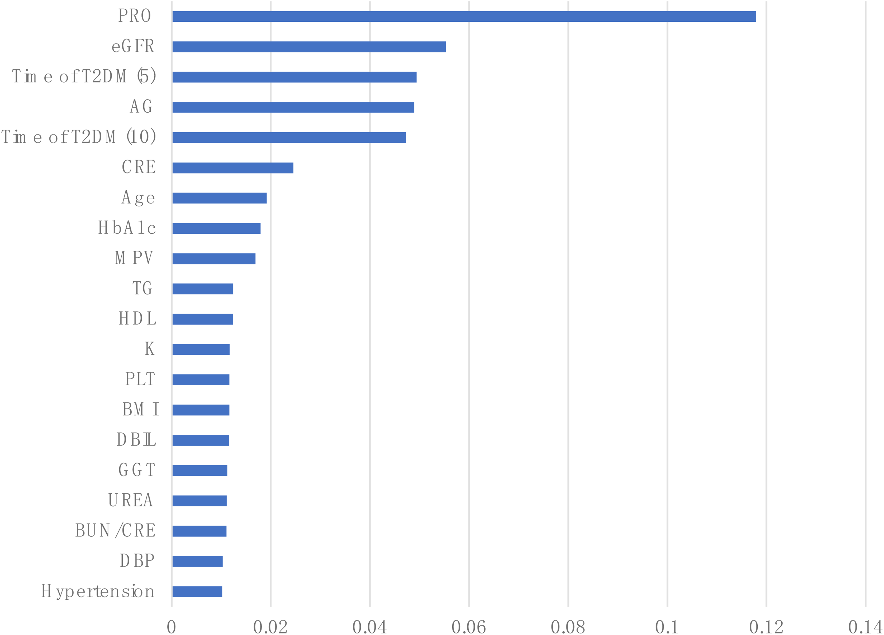
The importance of the top 20 features.

Table 4.

The results of feature importance.

Part 1		Part 2		Part 3
Features	Importance	Features	Importance	Features	Importance
PRO	0.11788	CO₂	0.01659	G	0.00837
eGFR	0.05534	RDW-CV	0.01634	Using insulin	0.00803
Time of T2DM (5)	0.04943	M%	0.01460	GLU	0.00772
AG	0.04892	L%	0.01421	HYC	0.00762
Time of T2DM (10)	0.04725	Ca	0.01387	LDL	0.00759
CRE	0.02458	TBIL	0.01359	Other kidney diseases	0.00753
Age	0.01919	IBIL	0.01356	CK	0.00742
HbA1c	0.01794	MCHC	0.01325	Cl	0.00739
MPV	0.01694	RDW-SD	0.01260	SBP	0.00722
TG	0.01240	L	0.01244	M	0.00717
HDL	0.01236	α-HBDH	0.00704	AST/ALT	0.00698
K	0.01172	Glycemic control	0.00690	UA	0.00690
PLT	0.01167	WBC	0.00679	P	0.0067
BMI	0.01162	TP	0.00631	EO	0.00595
DBIL	0.01157	N%	0.00594	ALP	0.00576
GGT	0.01120	ALB	0.00528	BASO%	0.00507
Urea	0.01109	N	0.00462	CK-MB	0.00431
BUN/CRE	0.01104	HGB	0.00394	BASO	0.00382
DBP	0.01032	SG	0.00266	Smoke	0.00250
Hypertension	0.01018	Urine pH	0.00180	Heredity	0.00160
A/G	0.01018	Drink	0.00132	Gender	0.00119
RBC	0.01005	Basic disease	0.00022
HCT	0.00998
LDH	0.00989
MCV	0.00972
MCH	0.00963
PDW	0.00959
ChE	0.00935
ALT	0.00934
EO%	0.00925
AST	0.00889
Na	0.00868
OSM	0.00853

eGFR: estimated glomerular filtration rate; T2DM: diabetes mellitus type 2; CRE: creatinine; HbA1c: hemoglobin A1c; MPV: mean platelet volume; TG : triglyceride; HDL: high density lipoprotein cholesterol; PLT: platelet; BMI: body mass index; DBIL: direct bilirubin; GGT: γ-glutamyltransferase; BUN/CREA: blood urea/creatinine; ChE: cholinesterase; HYC: homocysteine; PDW: platelet distribution width; SBP: systolic blood pressure; DBP: diastolic blood pressure; WBC: white blood cell count; RBC: red blood cell count; HGB: hemoglobin; ALT: aminotransferase; AST: aminotransferase; CK: creatine kinase; AFU: α-L-fucosidase; OSM: osmolality.

Handling class imbalance

Any two features in the training set were selected, and the visualization of the distributed predictions before and after the equalization of the dataset is run is shown in Figure 9. A few classes (class 0) have almost the same amount of data as class 1 after balancing is run.

Figure 9.

The distribution of the data before and after SMOTEomek resampling.

ROC curve

The ROC curves of the MLMs are shown in Figures 10 and 11. The AUC values of the training and validation curves for each model are close, indicating that each model has good generalization ability. Both specificity and AUC values were obtained.

Figure 10.

The ROC curve of the training set. (a) ROC curve of ensemble model. (b) ROC curve of Naive Bayes. (c) ROC curve of RF. (d) ROC curve of Cat-Boost. (e) ROC curve of XG-Boost. (f) ROC curve of Ada-Boost. (g) ROC curve of GBDT. (h) ROC curve of KNN. (i) ROC curve of DNN. (j) ROC curve of Light-GBM. (k) ROC curve of SVM. (l) ROC curve of LR.

Figure 11.

The ROC curve of the validation set. (a) ROC curve of ensemble model. (b) ROC curve of Naive Bayes. (c) ROC curve of RF. (d) ROC curve of Cat-Boost. (e) ROC curve of XG-Boost. (f) ROC curve of Ada-Boost. (g) ROC curve of GBDT. (h) ROC curve of KNN. (i) ROC curve of DNN. (j) ROC curve of Light-GBM. (k) ROC curve of SVM. (l) ROC curve of LR.

Ensemble model

We selected RF and NB for the components of the ensemble model based on their complementary performance characteristics observed in our experiments. As shown in Table 5, the NB classifier achieved the highest precision (100.00%) among all individual models, but its recall was comparatively lower (87.76%). In contrast, RF achieved the highest recall (97.96%) but had a relatively lower precision (76.19%). This suggests that NB is more conservative and accurate when it predicts a positive class, whereas RF is more comprehensive in capturing positive samples but may introduce more false positives.

Table 5.

Performance comparison of the classification models.

Models	Set	Accuracy %	Precision %	Recall %	F1 score	Specificity %	AUC
Ensemble model	Training set	99.17	100	97.83	98.9	100	1
Ensemble model	Validation set	97.62	100	95.92	97.92	99.32	0.95
Naive Bayes	Training set	98.33	100	95.74	97.83	100	1
Naive Bayes	Validation set	92.86	100	87.76	93.48	97.96	0.95
RF	Training set	98.25	100	95.45	97.67	100	1
RF	Validation set	80.95	76.19	97.96	85.71	63.94	0.93
Cat-Boost	Training set	100	100	100	100	100	1
Cat-Boost	Validation set	86.9	86.54	91.84	89.11	81.96	0.95
XG-Boost	Training set	100	100	100	100	100	1
XG-Boost	Validation set	85.71	84.91	91.84	88.24	79.58	0.94
Ada-Boost	Training set	100	100	100	100	100	1
Ada-Boost	Validation set	83.33	80.7	93.88	86.79	72.78	0.93
GBDT	Training set	100	100	100	100	100	1
GBDT	Validation set	80.95	78.95	91.84	84.91	70.06	0.93
KNN	Training set	87.5	100	75	85.71	100	1
KNN	Validation set	80.95	80	89.8	84.62	72.1	0.89
DNN	Training set	100	100	100	100	100	1
DNN	Validation set	79.76	77.59	91.84	84.11	67.68	0.9
Light-GBM	Training set	100	100	100	100	100	1
Light-GBM	Validation set	77.38	75	91.84	82.57	62.92	0.94
SVM	Training set	100	100	100	100	100	1
SVM	Validation set	75	71.88	93.88	81.42	56.12	0.92
LR	Training set	97.65	98.8	96.47	97.62	98.83	1
LR	Validation set	73.81	70.77	93.88	80.7	53.74	0.92
CSM	Training set	84.76	87.21	84.27	85.71	0.96	0.939
CSM	Validation set	84.88	87.5	85.71	86.6	0.948	0.765

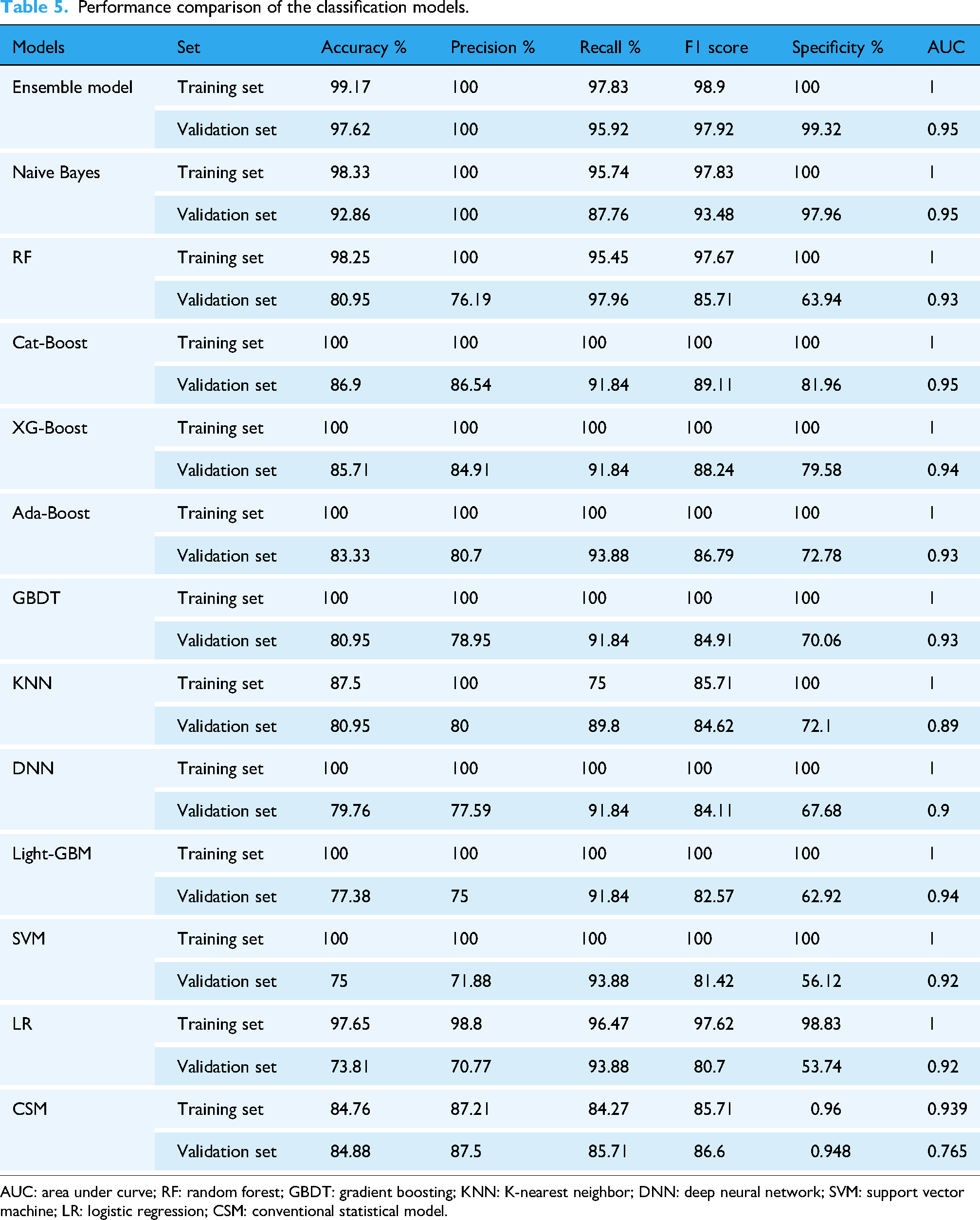
AUC: area under curve; RF: random forest; GBDT: gradient boosting; KNN: K-nearest neighbor; DNN: deep neural network; SVM: support vector machine; LR: logistic regression; CSM: conventional statistical model.

The fusion of RF and NB was therefore considered to balance these strengths, leveraging the high precision of NB and the high recall of RF, to achieve a more robust and stable classification outcome. This approach aligns with common ensemble learning principles, where combining diverse models with complementary strengths can yield improved overall performance.^16,17

Comparison of prediction models

The summary performance of all models is shown in Table 5. The predictive performance between the training set and the validation set is not significantly different for the first three models regarding machine learning models, but significantly different for the latter few models. However, the AUC curves of all models are not significantly different from each other and the values are quite impressive. The prediction performance between the training set and the validation set does not differ significantly in the traditional model. However, the difference in AUC between the two is much larger than that of machine learning. This indicates that the constructed model based on the traditional methods has a slightly weaker generalization ability and poor stability after LASSO regression regularization and secondary screening of influencing factors. Hosmer and Lemeshow's goodness of fit test gives rise to a good fit. Therefore, the significant difference in AUC between the two may be due to the retention of too many influencing factors. However, this article aims to identify as many indicators as possible to predict early DKD and provide new indicators and models. For clinical selection, two groups of methods were compared at the same level. Therefore, to maintain consistency in experimental objectives, methodology should be kept dominant as much as possible, while also ensuring that the results have clinical significance.

Because the validation set can better represent the actual performance of the model in clinical practice. So this experiment compares the predictive performance of two methods based on the validation set. The ensemble model outperforms all models in terms of performance. However, the CSM performs poorly in terms of AUC values. Compared to various MLMs, the performance of others is not inferior.

Discussion

Two different types of modeling tools, which are conventional and machine learning, are implemented and compared in the article.

When the screening of independent variables is under consideration, CSMs are very different from MLMs. MLMs sorted out all factors based on importance criteria and then included the top 20 factors as the independent attributes based on their importance scores. The CSMs first execute univariate analysis and remove the factors not statistically significant between the two groups. In many cases, due to small sample sizes, group differences not found to be statistically significant are removed. However, MLMs are not greatly affected by the issue. For example, the outcomes generated by Hu et al.,¹⁸ Yang and Jiang,¹⁹ and Hukportie et al.²⁰ suggested that DBP and BMI are related to diabetic nephropathy. However, this article suggested that DBP and BMI are directly excluded from the CSM since they are not statistically significant, while BMI and DBP were retained in the MLM and employed as independent variables to construct the model. CSMs in the second screening stage of variables and model fitting suggest that the PRO and eGFR are two indicators used in the model. Hosmer and Lemeshow's goodness of fit test shows a statistically significant relation since the p-value is < 0.05. However, the model fit is not good, so they are excluded. However, studies^6,21–24 suggested that eGFR and urinary protein have a strong correlation with diabetes. This article suggests that the two indicators, PRO and eGFR, have a strong correlation with the disease, which is much more related than other indicators, however, when these two indicators are included in the CSM, the model fitting will be poor. On the other hand, MLMs do not have this issue. Overall, MLMs as modeling tools are superior to CSMs when filtered-out variables are a concern. However, MLMs have this shortcoming. In the article, a set of similar variables, the history of T2DM (5) and the history of T2DM (10), are designed. The CSM well eliminated one group, while the MLM included both groups in the variable selection process.

Since the number of independent variables is limited in the model fitting stage, Riley et al.²⁵ suggested that the CSM has limitations due to the sample size. Hence insufficient sample size can also lead to poor fit of the model or affect the predictive performance of the model. Only nine variables are included in the CSM due to these limitations. However, MLMs included 20 variables.

Most studies implementing the CSMs^26–32 suggested that the sample sizes of the two groups are roughly equal or can be slightly different, but the difference should not be large, which will have a great impact on the prediction performance of the model when data balance between the two groups are a concern. However, the prediction performance is better after running handling class imbalance when MLMs are implemented.^33–35 Therefore, the significance of the process of handling class imbalance is underlined.

The CSM tool is easy to operate, learn, understand, and interpret. However, there are few modeling methods available for CSMs. On the other hand, the toolset of MLMs has several options to model. Only one modeling method in CSMs is implemented in the research. When compared with CSMs, MLMs are cumbersome operationally. Thus, they do not have the mentioned favorable features of what the CSM tool has.

Based on predictive performance, CSMs have good predictive performance compared to various MLMs, except for slightly lower AUC.

Overall, in a small sample size, CSMs and MLMs have their advantages and disadvantages. We cannot determine which one is better just because of the limited results of this experiment. Therefore, multiple comparisons should be made under different conditions. Both have their advantages and disadvantages and if their respective strengths can be retained and their shortcomings eliminated, it would be a good direction to be implemented. This article applies machine learning methods to integrate two MLMs into an ensemble model whose predictive performance is excellent.

At present, there are also applications of fused models in medical research, and their predictive performance is also very promising. Lu et al.³⁶ proposed a gate recurrent unit (GRU) and decision tree-based fusion model, and the accuracy of the fusion model was 98.31% and the precision was 96.73%. Khalid et al.³⁷ suggested that stacked classifiers were applied to construct a stacked model that combined gradient boosting, Gaussian NB, and RF, and the stacked model achieved 100% accuracy. Even though the proposed fusion model has higher accuracy and precision, its usability and practicality need to be tested in medicine. More research is needed to further verify the results of the proposed method.

This article applies multiple methods to establish a prediction model for ES-DKD. These models are all constructed based on commonly used testing indicators for clinical patients. During the modeling process, statistical methods were used to screen each indicator, leaving behind indicators with differences. Each model can be integrated with clinical practice. Extracting patient-related indicators through different models helps predict the risk of T2DM patients transitioning to ES-DKD. Due to different patient databases selected for model construction, the different indicators applied to the models established by different databases are found. Therefore, it cannot be said that the excluded indicators cannot be regarded to predict the disease, but can only indicate that there is no difference in the indicators between the two groups in the databases and, therefore they were not used to establish a model. Consequently, this model still has some limitations.

There are also some limitations to the research. The first point is that although this experiment aims to explore the comparison of two modeling methods under small sample sizes, the used sample size is too small. Secondly, in this experiment, due to the actual situation of the patients, the vast majority of them have some underlying diseases. This is in line with the current clinical situation, so it is impossible to avoid the impact of these potential diseases on the indicators. For example, diabetes or DKD may be improved while treating other basic diseases. When angiotensin-converting enzyme inhibitors (ACEIs) are used to treat hypertension, proteinuria is also treated, thereby reducing kidney function damage. This situation may affect the generalization ability of the model. Thirdly, all models established in this article have only been validated on the validation set and have not been clinically tested. Therefore, the practical application performance of the model in clinical practice still needs to be examined. The fourth point is that although the training set and validation set come from different hospitals, both hospitals are located in the same region. Therefore, the model established only has good predictive ability in that region but lacks generalization capability testing in different regions. The fifth point is that when establishing the model, there may be a risk of overfitting as a small number of indicators overlap with the patient's diagnostic indicators. In summary, this study should fully consider the aforementioned limitations and attempt to find solutions to these issues, so that the constructed model can be widely applied in clinical practice without affecting the aforementioned limitations.

Conclusion

This article establishes multiple ES-DKD prediction models using CSMs and MLMs to find some new routine clinical laboratory indicators that can be used for prediction. This provides new ideas and methods for the diagnosis, treatment, and prevention of ES-DKD in clinical practice, especially with the popularization and application of AI today. Mathematical models can be better applied in clinical practice and closely integrated with clinical practice. However, models built with different databases may have limitations due to geographical and special conditions, so newly established models need to be continuously improved in practical application and testing.

This article also compared two modeling methods. Compared to CSMs, MLMs have good stability and varying predictive abilities. Therefore, when applying MLMs for modeling, several different methods should be used to select the best one. The CSMs have relatively fixed modeling methods. However, compared to MLMs, the operation is simple and convenient. The predictive ability is also very good. This article also established an integrated model, which has excellent predictive capability, stability, and generalization capability. Therefore, fusion models will be the main research direction for future mathematical models. However, building a fused model is quite cumbersome. On the other hand, the integration of the advantages of MLMs based on CSMs would bring more promising outcomes.

Footnotes

ORCID iD

Xiaoqin Ha

Ethics considerations

The study protocol was approved by the 940th Hospital of the Joint Logistics Support Force of the Chinese People's Liberation Army's Ethics Committee (Ethical reference: 2022KYLL170). The study protocol was approved by the First Hospital of Lanzhou University Ethics Committee (Ethical reference: LDYYLL-2024-368).

Consent to participate

I promise to strictly follow the declaration of Helsinki, and each patient signed the informed consent.

Author contributions

YS and JC participated in the design of the experimental study, proposed the experimental protocol, and searched the literature. YS, JC, and CZ completed the preliminary writing of the manuscript. CZ, YS, JC, FM, QX, DW, and JZ collected, organized, and analyzed the data. HX, as the corresponding author, guided and improved the experimental design and protocol. All authors reviewed the article.

Funding

The authors disclosed receipt of the following financial support for the research, authorship, and/or publication of this article: This project is funded by the Fund of Gansu Provincial Health Commission of China [Approval No.: GSWSKY2022-03]. The funder does not play any role in research design, data collection and analysis, publishing decisions, or manuscript preparation.

Declaration of conflicting interests

YS and JC are co first authors with consistent contributions to this article. There are no potential conflicts of interest in other aspects.

Guarantor

Yingda Sheng.

References

International Diabetes Federation. IDF diabetes atlas. 10th ed. Brussels, Belgium, 2021. https://www.diabetesatlas.org .

Xie

Jin

Qiu

, et al. Assessment of urinary podocalyxin as an alternative marker for urinary albumin creatinine ratio in the early stage of diabetic kidney disease in older patients. Nefrologia (Engl Ed) 2022; 42: 664–670.

Zhang

Long

Jiang

, et al. Trends in chronic kidney disease in China. N Engl J Med 2016; 375: 905–906. doi:10.1056/NEJMc1602469

Jiang

Zhang

. Construction and verification of predictive model for influencing factors of quality of life in patients with type 2 diabetic nephropathy: a hospital-based retrospective study. Arch Esp Urol 2023; 76: 418–424.

Zhang

Liu

Dong

, et al. New diagnostic model for the differentiation of diabetic nephropathy from non-diabetic nephropathy in Chinese patients. Front Endocrinol (Lausanne) 2022; 13: 913021. Published 2022 Jun 30.

Oshima

Shimizu

Yamanouchi

, et al. Trajectories of kidney function in diabetes: a clinicopathological update. Nat Rev Nephrol 2021; 17: 740–750.

Expert Group of Nephrology Branch of Chinese Medical Association. Chinese Guidelines for diagnosis and treatment of diabetic kidney disease. Chin J Nephrol 2021; 37: 255–304.

Kidney Disease: Improving Global Outcomes (KDIGO) Lupus Nephritis Work Group. KDIGO 2024 Clinical practice guideline for the management of lupus nephritis. Kidney Int 2024; 105: S1–S69.

Gansevoort

Anders

Cozzolino

, et al.

What should European nephrology do with the new CKD-EPI equation?

Nephrol Dial Transplant 2023; 38: 1–6.

10.

Delanaye

Cavalier

Pottel

, et al. New and old GFR equations: a European perspective. Clin Kidney J 2023; 16: 1375–1383. Published 2023 Mar 15.

11.

American Diabetes Association. Microvascular complications and foot care: standards of medical care in diabetes-2020. Diabetes Care 2020; 43: S135–S151.

12.

Breiman

. Random forests. Mach Learn 2001; 45: 5–32.

13.

Díaz-Uriarte

Alvarez de Andrés

. Gene selection and classification of microarray data using random forest. BMC Bioinformatics 2006; 7: 1–13.

14.

Genuer

Poggi

Tuleau-Malot

. Variable selection using random forests. Pattern Recognit Lett 2010; 31: 2225–2236.

15.

Kursa

Rudnicki

. Feature selection with the Boruta package. J Stat Softw 2010; 36: 1–13.

16.

Rokach

. Ensemble-based classifiers. Artif Intell Rev 2010; 33: 1–39.

17.

Kuncheva

. Combining pattern classifiers: methods and algorithms. Oxford, UK: John Wiley & Sons, 2014.

18.

Shi

, et al. Nomogram for the prediction of diabetic nephropathy risk among patients with type 2 diabetes mellitus based on a questionnaire and biochemical indicators: a retrospective study. Aging (Albany NY) 2020; 12: 10317–10336.

19.

Yang

Jiang

. Development and validation of a model that predicts the risk of diabetic nephropathy in type 2 diabetes mellitus patients: a cross-sectional study. Int J Gen Med 2022; 15: 5089–5101.

20.

Hukportie

Zhou

, et al. Anthropometric measures and incident diabetic nephropathy in participants with type 2 diabetes mellitus. Front Endocrinol (Lausanne) 2021; 12: 706845. Published 2021 Aug 4.

21.

Selby

Taal

. An updated overview of diabetic nephropathy: diagnosis, prognosis, treatment goals and latest guidelines. Diabetes Obes Metab 2020; 22: 3–15.

22.

Hosseini Sarkhosh

Hemmatabadi

Esteghamati

. Development and validation of a risk score for diabetic kidney disease prediction in type 2 diabetes patients: a machine learning approach. J Endocrinol Invest 2023; 46: 415–423.

23.

Zou

Zhao

Zhang

, et al. Development and internal validation of machine learning algorithms for end-stage renal disease risk prediction model of people with type 2 diabetes mellitus and diabetic kidney disease. Ren Fail 2022; 44: 562–570.

24.

Jiang

Wang

Shen

, et al. Establishment and validation of a risk prediction model for early diabetic kidney disease based on a systematic review and meta-analysis of 20 cohorts. Diabetes Care 2020; 43: 925–933.

25.

Riley

Ensor

Snell

KIE

, et al. Calculating the sample size required for developing a clinical prediction model. Br Med J 2020; 368: m441. Published 2020 Mar 18.

26.

Saito

Tanabe

Kudo

, et al. A high FIB4 index is an independent risk factor of diabetic kidney disease in type 2 diabetes. Sci Rep 2021; 11: 11753. Published 2021 Jun 3.

27.

Zhou

Chen

, et al. Relationship between the TyG index and diabetic kidney disease in patients with type-2 diabetes mellitus. Diabetes Metab Syndr Obes 2021; 14: 3299–3306. Published 2021 Jul 17.

28.

Sanchez-Alamo

Shabaka

Cachofeiro

, et al. Serum interleukin-6 levels predict kidney disease progression in diabetic nephropathy. Clin Nephrol 2022; 97: 1–9.

29.

Wang

Chang

Zhao

, et al. Glutathione peroxidase 4 is a predictor of diabetic kidney disease progression in type 2 diabetes mellitus. Oxid Med Cell Longev 2022; 2022: 2948248. Published 2022 Oct 12.

30.

Sun

Chang

, et al. C3c deposition predicts worse renal outcomes in patients with biopsy-proven diabetic kidney disease in type 2 diabetes mellitus. J Diabetes 2022; 14: 291–297.

31.

Zhou

Shen

, et al. Severe 25-hydroxyvitamin D deficiency may predict poor renal outcomes in patients with biopsy-proven diabetic nephropathy. Front Endocrinol (Lausanne) 2022; 13: 871571. Published 2022 May 4.

32.

Gao

Feng

Yang

, et al. Development and external validation of a nomogram and a risk table for prediction of type 2 diabetic kidney disease progression based on a retrospective cohort study in China. Diabetes Metab Syndr Obes 2022; 15: 799–811. Published 2022 Mar 14.

33.

Wang

Tian

Zheng

, et al. Improving risk identification of adverse outcomes in chronic heart failure using SMOTE+ENN and machine learning. Risk Manag Health Policy 2021; 14: 2453–2463. Published 2021 Jun 8.

34.

Wang

. Prediction of postoperative recovery in patients with acoustic neuroma using machine learning and SMOTE-ENN techniques. Math Biosci Eng 2022; 19: 10407–10423.

35.

Alghamdi

Al-Mallah

Keteyian

, et al. Predicting diabetes mellitus using SMOTE and ensemble machine learning approach: the Henry Ford exercise testing (FIT) project. PLoS One 2017; 12: e0179805. Published 2017 Jul 24.

36.

Zhang

Zhou

, et al. Identification of arrhythmia by using a decision tree and gated network fusion model. Comput Math Methods Med 2021; 2021: 6665357. Published 2021 May 29.

37.

Khalid

Khan

Zahid Khan

, et al. Machine learning hybrid model for the prediction of chronic kidney disease. Comput Intell Neurosci 2023; 2023: 9266889. Published 2023 Mar 14.

Establishment and comparison of prediction models for early-stage diabetic kidney disease

Abstract

Background

Objective

Methods

Results

Conclusion

Keywords

Introduction

Methodology

The objective of the research

Methods

Indicators

Modeling based on conventional statistical methods

Modeling based on machine learning methods

Results

Results of the CSMs

Univariate statistics

Screening of independent variables

The construction of the logistic regression model and nomogram

ROC curve, calibration curve, and DCA

The results of machine learning models

Feature selection

Handling class imbalance

ROC curve

Ensemble model

Comparison of prediction models

Discussion

Conclusion

Footnotes

ORCID iD

Ethics considerations

Consent to participate

Author contributions

Funding

Declaration of conflicting interests

Guarantor

References