Sage Journals: Discover world-class research

Abstract

Objective

Hepatitis B virus (HBV) is a significant global health threat, responsible for severe liver diseases such as liver failure, cirrhosis, and hepatocellular carcinoma. The burden is especially high in low-income regions, where early diagnosis and treatment are critical for mitigating its impact. This study investigates the effectiveness of various machine learning (ML) techniques in predicting patient outcomes in HBV infection.

Methods

The Chi-squared test was used for feature selection to find the most important factors, which were later applied to train and evaluate various ML models. To address the class imbalance in the dataset, the Synthetic Minority Over-sampling Technique (SMOTE) was used to balance the data. SHapley Additive exPlanations (SHAP) and Local Interpretable Model-agnostic Explanations (LIME) were used to improve the models’ interpretability.

Results

Among individual models, Support Vector Machine (SVM) and Logistic Regression (LR) each achieved an accuracy of 92.5%. By implementing a Voting Classifier that combined SVM and LR, the overall accuracy was improved to 95%. The results showed that higher levels of some risk factors, especially in older patients, greatly raise the risk of death.

Conclusion

These insights provide healthcare professionals and policymakers with valuable information to develop predicting better patient outcomes in HBV infection and patient care strategies.

Keywords

Hepatitis B risk factors artificial intelligence model explainability

Introduction

Hepatitis B virus (HBV) is a major global health concern, infecting over 257 million people and contributing to liver cirrhosis, liver failure, and hepatocellular carcinoma.¹ The virus is primarily transmitted through blood, unprotected sexual contact, and perinatal transmission, with the highest prevalence in Africa (6.1%) and the Western Pacific (6.2%).² Although vaccination has significantly reduced new infections in some regions, chronic HBV remains a leading cause of liver-related mortality. The virus infects liver cells by binding to specific receptors, integrating into the host genome, and triggering immune-mediated liver damage. While some individuals clear the infection naturally, others develop chronic HBV, which progresses silently for years before leading to severe complications. A major challenge in HBV management is the difficulty in early diagnosis and prognosis, as many infected individuals remain asymptomatic, delaying treatment and increasing the risk of severe liver damage. Current diagnostic methods rely on biochemical markers and virological tests, but they fail to accurately predict disease progression and patient outcomes. Traditional statistical models struggle with high-dimensional clinical data, limiting their effectiveness. This study addresses these challenges by leveraging ML techniques to improve early detection, outcome prediction, and model interpretability using SHAP and LIME. By integrating feature selection and data balancing, this research enhances the accuracy and transparency of HBV prognosis, aiding clinicians in better decision-making. Figure 1 shows the symptoms of the HBV.

Figure 1.

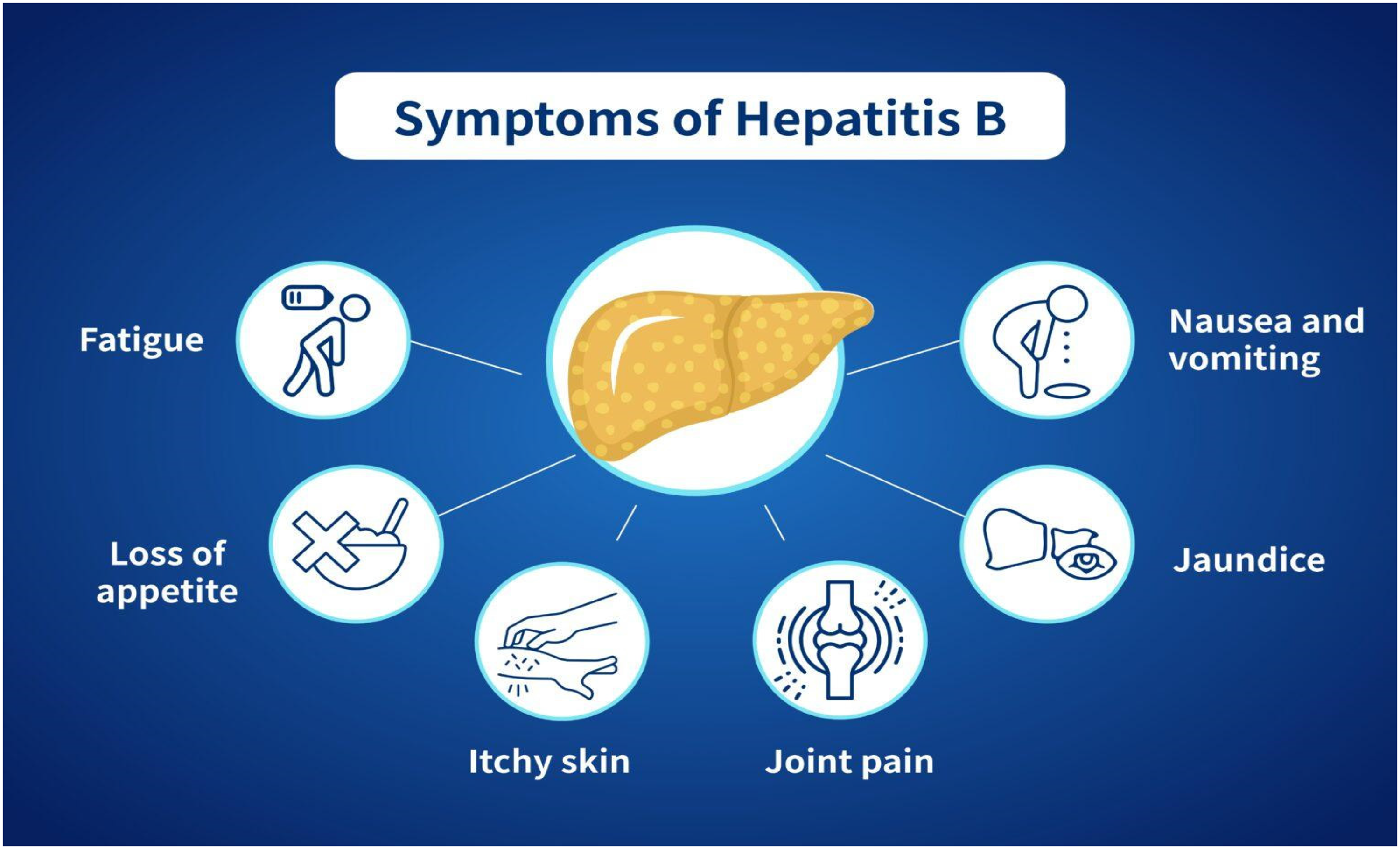
Symptoms of HBV.

Several studies have applied ML techniques for HBV diagnosis, prognosis, and prediction of patient outcomes, using both real-world patient records and publicly available datasets. Tian et al.³ explored ML-based prognosis on 2235 real patient records, where XGBoost achieved the highest AUC of 0.891. Obaido et al.⁴ applied SHAP for interpretability on the UCI Hepatitis dataset (155 patients), with AdaBoost attaining 92% accuracy and identifying bilirubin as a key predictor. Yarasuri et al.⁵ also used the UCI dataset, where ANN achieved 96% accuracy. Putri et al.⁶ addressed data imbalance in a real-world dataset of 2264 patient records, improving Naïve Bayes’ accuracy to 73.22% using SMOTE. Alamsyah et al.⁷ applied PCA with SVM, enhancing hepatitis diagnosis to 93.55% accuracy. Albogamy et al.⁸ employed BiLSTM deep learning, achieving 95.08% accuracy in predicting survival. Chen et al.⁹ used Random Forest with sequence-based features, obtaining 90% accuracy in hepatocellular carcinoma prediction. Peng et al.¹⁰ developed an explainable AI (XAI) framework, where Random Forest reached 91.9% accuracy, improving model transparency. These studies highlight ML's potential for HBV classification, but challenges in dataset size, model interpretability, and clinical applicability remain.

While previous studies have demonstrated the potential of ML in HBV diagnosis and prognosis, they often face some problems and a lack of techniques like feature selection, class imbalance handling, and model interpretability. Most studies did not incorporate feature selection, leading to models trained on redundant or less relevant features. Class imbalance was another challenge, as minority-class outcomes (e.g., mortality cases) were underrepresented, potentially skewing predictions. Furthermore, while some studies integrated explainability techniques like SHAP and LIME, many ML models remained “black boxes,” making it difficult for clinicians to interpret results. To overcome these challenges, this study employs Chi-squared feature selection to identify the most relevant factors influencing HBV outcomes, improving model efficiency. This research addresses class imbalance using SMOTE, ensuring a more balanced dataset for training. Unlike prior studies that evaluated multiple models individually, this project utilizes an ensemble Voting Classifier (SVM + LR), which achieves 95% accuracy, surpassing existing approaches. Additionally, this research integrates SHAP and LIME to enhance model transparency, offering interpretable insights for clinical decision-making.

This study aims to develop an ML-driven predictive framework for assessing mortality risk in HBV-infected patients, enabling early detection, risk stratification, and improved clinical decision-making. The dataset consists of 20 clinical and biochemical features, allowing for a comprehensive analysis of risk factors influencing patient outcomes. To enhance model reliability, this research evaluates multiple ML algorithms, including SVM, LR, Decision Trees, Random Forest, Gaussian Naïve Bayes, K-nearest neighbor (KNN), Light-GBM (LGBM), AdaBoost, Cat-Boost, and ensemble learning methods. Performance is assessed using accuracy, precision, recall, F1-score, and AUC, ensuring robust validation and generalizability. A key focus of this study is bridging the gap between model accuracy and clinical interpretability. To achieve this, this research integrates SHAP and LIME, providing explainable AI insights into how specific clinical variables influence the model's predictions. By leveraging feature selection (Chi-squared test) and class balancing (SMOTE), this project ensures that the model is optimized for real-world medical use. Ultimately, this research aims to develop a highly accurate, transparent, and clinically practical ML model that can assist healthcare professionals in identifying high-risk HBV patients and guiding timely interventions.

Materials and methods

This section provides a comprehensive overview of the techniques and resources utilized in this study. The process began with importing the HBV dataset, followed by data preprocessing, where missing numerical values were handled using the median, and duplicate rows were checked. Feature selection was conducted using the Chi-squared (Chi2) test, and SMOTE was applied to address the class imbalance. The dataset was scaled before training and testing different ML models. Performance analysis was carried out using metrics such as the confusion matrix and ROC curve. Additionally, model explainability was explored using SHAP and LIME techniques. Figure 2 shows the workflow of the proposed method for diagnosing HBV.

Figure 2.

Workflow of the proposed methodology.

Dataset preparation

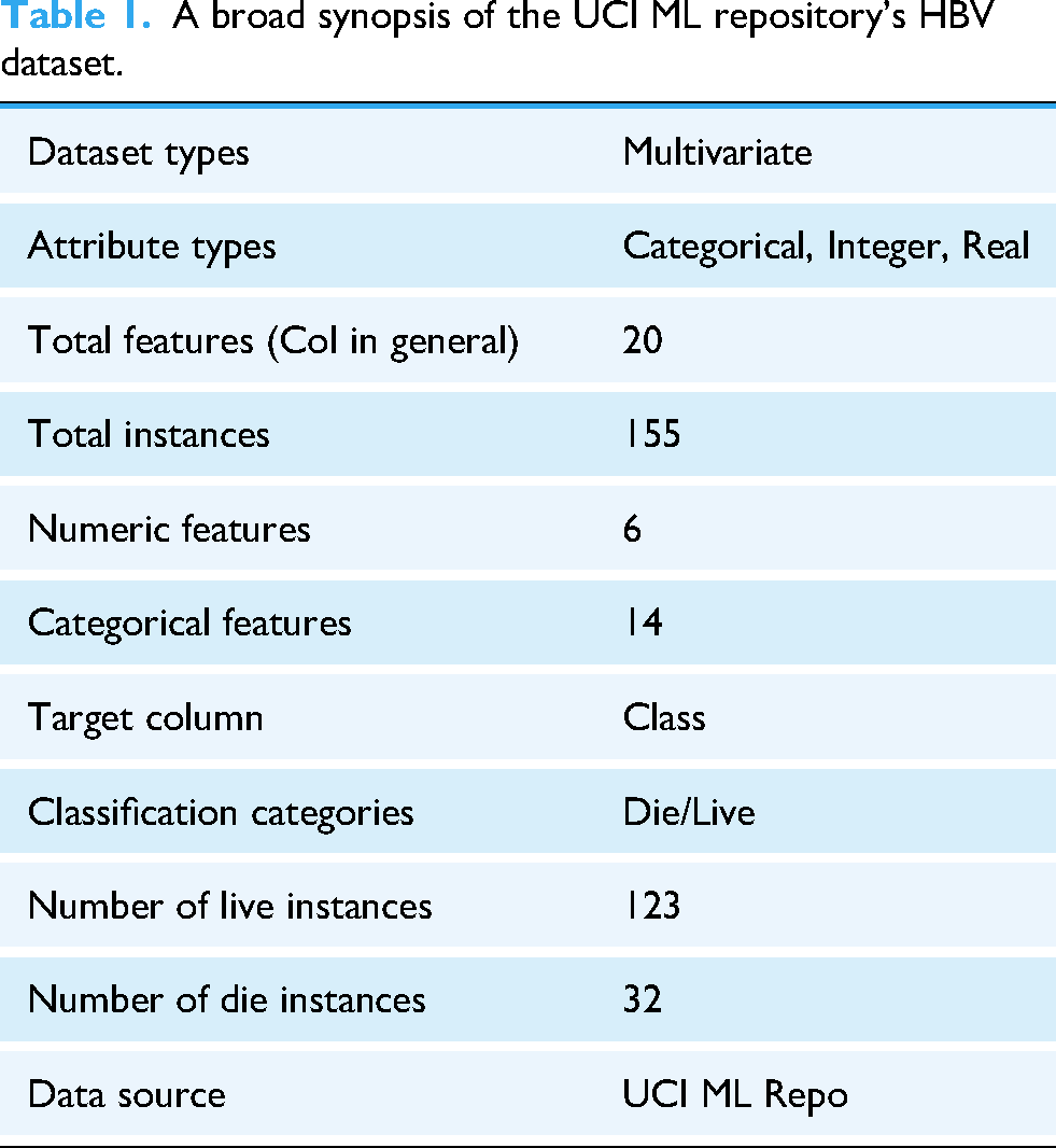
The dataset used in this study was sourced from the University of California Irvine (UCI) Machine Learning Repository,¹¹ selected due to its established role in providing curated datasets for the ML community. Table 1 provides a summary of the dataset's features. The choice to use hepatitis datasets from this repository was made deliberately, given the limited availability of relevant data in this area of research. The dataset includes demographic and clinical information for 155 Hepatitis B patients, encompassing 20 distinct features.

Table 1.

A broad synopsis of the UCI ML repository's HBV dataset.

Dataset types	Multivariate
Attribute types	Categorical, Integer, Real
Total features (Col in general)	20
Total instances	155
Numeric features	6
Categorical features	14
Target column	Class
Classification categories	Die/Live
Number of live instances	123
Number of die instances	32
Data source	UCI ML Repo

To prevent data leakage, the dataset was first checked for duplicate samples, but none were found. Missing data were addressed using the fillna method, which handled 167 missing values across 20 features in a dataset of 155 records. The missing values were imputed with the median using the fillna technique, replacing the NULL values with specified values. After feature selection, the top 80% of the most important features were selected for further analysis. The dataset had an issue of imbalance, where one class had significantly fewer instances compared to the other, which could negatively impact the performance of ML models. To tackle this issue, SMOTE¹² was used to create synthetic samples for the minority class, which helped balance the dataset. Additionally, the dataset was scaled using a standardization scaling method, which transformed the features to have a mean of zero and a standard deviation of one. This ensured that all features remained on the same scale, preventing any feature from dominating the model due to larger values, and improving the overall model performance. Table 2 summarizes the dataset, outlining each variable along with its type, and small description. The features were further standardized using the Z-score scaling method.¹³ In Eq. (1), X represents the original values, while $μ$ and $σ$ denote the mean and standard deviation of the feature $f_{i}$ , respectively. The standardized values are denoted as Z, with the following equation:

Z = \frac{X - μ}{σ}

(1)

where

X, μ, σ \in f_{i}

. This process ensures that all features have an equal impact on the analysis, enhancing the performance of ML algorithms. After scaling the dataset, 80% was set aside for training, and the remaining 20% was kept for testing.

Table 2.

Overall summary of the HBV dataset available in the UCI ML repository.

SL	Features	Description	Data type
1	Age	Age of the patient	Numerical
2	Sex	Patient's gender: Male or Female	Nominal
3	Steroid	Use of steroids, which may increase HBV replication	Nominal
4	Antivirals	Antiviral drugs to inhibit HBV replication	Nominal
5	Fatigue	Fatigue due to impaired functional capacity from HBV	Nominal
6	Malaise	General discomfort and unease	Nominal
7	Anorexia	Loss of appetite	Nominal
8	Liver Big	Presence of liver enlargement	Nominal
9	Liver Firm	Firmness of the liver	Nominal
10	Spleen Palpable	Palpable enlargement of the spleen	Nominal
11	Spiders	Unusual grouping of blood vessels closes to the skin's surface.	Nominal
12	Ascites	Build-up of fluid in the abdomen	Nominal
13	Varices	Swollen veins, commonly found in the esophagus or stomach	Nominal
14	Bilirubin	Yellowish pigment formed by red blood cell breakdown	Numerical
15	Alk Phosphate	Enzyme used to assess liver fibrosis levels	Numerical
16	Sgot	Liver enzyme indicating liver function	Numerical
17	Albumin	Protein produced by the liver	Numerical
18	Protime	Blood clotting protein produced by the liver	Numerical
19	Histology	Microscopic examination of liver tissue	Nominal
20	Class	Patient outcome: “Died” or “Lived"	Nominal

In the dataset, the number of patients with missing age data is with percentage of 0%. Also, the percentage of missing values for Bilirubin is 3.87%. The missing data percentage for Alk Phosphate is shown to be 18.71%. Then, the missing value percentage for SGOT is 2.58%. Additionally, the missing count for Albumin is 10.32%, while Protime has the highest missing value percentage at 43.23%. Figure 3 illustrates the distribution of the nominal features, along with the numeric of each attribute present in the dataset. The visualization reveals a class imbalance, which was addressed using SMOTE.

Figure 3.

provides a visual representation of the distribution of nominal features in the dataset.

Figure 3 presents the distribution of the nominal features in the dataset. The first figure shows the distribution of gender, with 139 males and 16 females. For steroids, 76 patients have “No,” 78 have “Yes,” and 1 value is missing. The antivirals count indicates 131 “Yes” and 24 “No.” Fatigue shows 54 “Yes,” 100 “No,” and 1 missing value. Malaise has 93 “Yes” and 61 “No,” with 1 missing entry. For Anorexia, 122 are “Yes,” 32 are “No,” and 1 is missing. Liver Big shows 120 “Yes,” 25 “No,” and 10 missing values. Liver Firm has 84 “Yes,” 60 “No,” and 11 missing values. Spleen Palpable counts 120 “Yes,” 30 “No,” and 5 missing values. For Spiders, 99 are “Yes,” 51 are “No,” and 5 are missing. Ascites has 130 “Yes” and 20 “No,” with 5 missing values. Varices show 132 “Yes,” 18 “No,” and 5 missing values. Histology counts 70 “Yes” and 85 “No,” with no missing data. Finally, the Class attribute has 123 “Live” and 32 “Die” cases, with no missing values.

Features selection

As highlighted by Qin et al. (2020),¹⁴ identifying the most critical risk factors in healthcare informatics can reduce the time required for ML algorithm training. Which improves data consistency, removes redundant features and increases prediction performance. In recent years, researchers have adopted multiple approaches for selecting relevant features, including the Chi2 test, Principal Component Analysis (PCA), Recursive Feature Elimination (RFE), and Mutual Information (MI). Among these methods, the Chi2 Test has emerged as a key approach for feature selection.

In this study, the Chi2 test was applied to identify the most important features of the dataset. The Chi2 test examines the statistical independence of each feature from the target variable, helping to identify those with the strongest association.¹⁵ Following the Chi2 test, the features were ranked by importance and the top 80% of the most important features were selected for further analysis. Eq. (2) defines $\in_{ω}$ , which represents the set of important features identified through the Chi2 test. This set contains features that have been deemed statistically significant based on their Chi2 values and their relevance to the target variable. x represents a feature from the dataset. After chi2 test, $\in_{ω}$ becomes $\in_{ω} = {P r o t i m e, B i l i r u b i n, A g e, A l k P h o s p a t e,$ $S p i d e r s, A l b u m i n, H i s t o l o g y, A s c i t e s,$ $F a t i g u e, M a l a i s e, V a r i c e s, S p l e e n P a l p a b l e,$ $S g o t, S e x, A n o r e x i a, A n t i v i r a l s}$

\in_{ω} = {x | x \in χ^{2}}

(2)

A Pearson correlation check was performed to identify highly correlated features, particularly those with a correlation coefficient exceeding 80%. However, no strongly correlated features were found. The Pearson correlation matrix, illustrated in Figure 4, visualizes the relationships between features.¹⁶

Figure 4.

Pearson correlation matrix of selected features.

Figure 4 represents the correlation matrix of the selected features identified after the feature selection process. The correlation values can vary from −1 to +1. A correlation value of 0 means there is no linear relationship between the two features. As the value gets closer to +1, it indicates a strong positive correlation, which means the features increase together. On the other hand, values near −1 suggest a strong negative correlation, where an increase in one feature corresponds with a decrease in the other, indicating an inverse relationship.

Machine learning models

With the use of data structures, ML models enable prediction systems to produce precise forecasts in a variety of fields, improving efficiency and decision-making. Regression and classification in clinical and health diagnosis involve the development of models based on historical analysis in both supervised and unsupervised learning methodologies. Ten classifiers—Decision Tree, Random Forest, Logistic Regression, Gaussian Naïve Bayes, Support Vector Machines, K-Nearest Neighbor, Light-GBM classifier, Ada Boost, Cat-Boost, and Voting—are used to evaluate the performance; these are all covered in this section. The best accurate model among these classifiers is then evaluated, indicating its superior performance.

Logistic regression

Logistic Regression, developed by David Cox in 1958, is a widely used statistical classification technique in biological and medical research.¹⁷ It models binary-dependent variables by estimating probabilities using the logistic function, making it useful for predicting outcomes like disease presence or absence.^18,19 LR establishes the relationship between predictor and dependent variables through regression coefficients, determining the probability of an event occurring, such as HBV presence.²⁰

Support vector machine

Support Vector Machine is a supervised learning algorithm widely used for classification and regression due to its ability to maximize the separation between data clusters.^21,22 It utilizes support vectors to define decision boundaries and employs kernel functions (e.g., linear, polynomial, and radial basis function) to map non-linearly separable data into a higher-dimensional space for better classification. By optimizing the margin between positive and negative instances, SVM ensures robust decision boundary computation, making it effective for complex data analysis.²³

Voting classifier

The Ensemble Voting Classifier is a meta-classifier that combines multiple ML classifiers to improve recognition and classification performance.²⁴ It utilizes both hard voting, where the majority class label is selected, and soft voting, which averages predicted probabilities for classification. Hard and soft voting methods are both applied in this study to enhance model robustness and accuracy.

Other used ML models

In this study, multiple other ML algorithms were explored to predict patient outcomes in HBV infection, with a focus on classification accuracy and interpretability. Decision Tree classifiers provided a transparent framework for identifying key decision rules from clinical features, though they were prone to overfitting in small datasets.^25–28 Random Forest addressed this limitation by aggregating multiple decision trees, improving generalization and stability in predicting survival outcomes.^29–31 Gaussian Naïve Bayes was applied for its simplicity and speed, offering rapid predictions from clinical inputs, though its assumptions led to reduced performance in the presence of correlated features.^32,33 K-Nearest Neighbor, which classifies patients based on similarity to others, offered intuitive predictions but showed sensitivity to noise and imbalanced classes.³⁴ Light Gradient Boosting Machine (LGBM) effectively handled high-dimensional data and delivered fast, accurate predictions by growing tree's leaf-wise and directly managing categorical inputs.³⁵ AdaBoost enhanced weak learners by iteratively focusing on misclassified instances, yielding a robust model that demonstrated strong performance despite limited data.^36–41 CatBoost further improved upon boosting techniques by handling categorical clinical features without one-hot encoding, making it particularly suitable for this medical dataset where feature preprocessing was minimal.

Model explainability techniques

Model explainability is essential in ML, especially in fields like healthcare and finance, where understanding decisions is critical. As models grow more complex, techniques like SHAP and LIME enhance transparency by explaining predictions. SHAP, based on game theory, assigns values to features, showing their impact on predictions, while LIME simplifies models by analyzing feature influence through input modifications. These methods improve debugging, bias reduction, and user trust, making ML models more reliable and fairer. As AI advances, SHAP and LIME will remain crucial for developing interpretable and trustworthy systems.

SHapley Additive exPlanations (SHAP)

SHAP is a state-of-the-art ML explainability tool based on cooperative game theory, used to analyze model performance across various ML architectures, including decision trees, gradient-boosted models (e.g., XGBoost, CatBoost), and random forests.^42,43 Different SHAP versions, such as Tree-based SHAP, Deep SHAP, and Kernel SHAP, are tailored for specific model types. SHAP values quantify each feature's contribution to a prediction, ensuring interpretability and consistency while distinguishing between positive and negative feature influences.^44,45 This method is applicable to both classification and regression problems, making it a versatile tool for model transparency.

Local Interpretable Model-agnostic Explanations (LIME)

LIME is a widely used ML explainability technique that provides local interpretability by approximating complex models with simpler, interpretable models around specific instances.⁴⁶ It is model-agnostic, meaning it can be applied to various ML algorithms, including classifiers and regressors, making it a versatile tool for transparency. LIME works by generating perturbed datasets around an instance and training a local surrogate model, which mimics the behavior of the original model within a limited region. The coefficients of the surrogate model highlight feature importance, offering insights into how individual predictions are made. This approach is particularly useful in high-stakes fields like healthcare and finance, where understanding model behavior is essential for trust and decision-making.

Environmental setup

The experiments were conducted under several conditions to obtain the results and the experimental setup is detailed in Table 3. All methods were implemented locally using Python, with tools such as Python notebooks and libraries like Matplotlib, NumPy, Pandas, Seaborn, and Scikit-Learn. The project code was implemented in Google Colab. The research was conducted at Dhaka International University, Bangladesh. The duration of the research was almost 6 months.

Table 3.

Specifications of the system for developing the ML model

CPU	1 × 11TH Gen Intel^®Core™i5- 1135G7 @ 2.40 GHz
RAM	8 GB
Cache	46 MB
GPU	Intel iRISX^e
GPU Memory	8 GB
Session Limit	10 h
Disk Space	256 GB

Performance matrix

A confusion matrix is a crucial tool for evaluating the performance of an ML model in classification tasks. It provides a summary of how well the model predicts categorical labels by comparing the actual and predicted values. The matrix consists of true positives (TP), false positives (FP), false negatives (FN), and true negatives (TN), which help assess the model's effectiveness. Several key evaluation metrics can be derived from the confusion matrix to measure performance. Accuracy represents the proportion of correctly classified instances, indicating the overall reliability of the model. Precision measures the percentage of correctly predicted positive cases, reflecting how well the model minimizes false positives. Recall, also known as sensitivity or the true positive rate, evaluates the model's ability to correctly identify actual positive cases. The F1 score combines precision and recall into a single metric, balancing the trade-off between them to provide a comprehensive assessment of model performance. A higher F1 score indicates a well-balanced model with strong predictive capabilities.⁴⁷

Additionally, various assessment criteria were employed to evaluate the effectiveness of the available ML classifiers. Here, TP, TN, FP, and FN represent true positive, true negative, false positive, and false negative, respectively. Test samples labeled as positive are considered true positives, while those classified as negative are termed false positives. A positive test sample is labeled as a false negative if it is a true negative, and a negative test sample is classified as a true negative if it is indeed negative. Furthermore, two key metrics used to demonstrate the success of ML algorithms are the receiver operating characteristic curve (ROC) and the area under the ROC curve (AUC). To better illustrate the performance of the ML models, we utilized both measures in this study. The AUC indicates the algorithm's ability to differentiate between healthy (positive) and sick (negative) individuals, as it represents the ROC curve, which graphs the true positive rate (TPR) against the false positive rate (FPR) at different threshold levels. A higher AUC value indicates better discrimination between the two classes.

Results

This section presents a thorough overview of the results of the study. The dataset was randomized and separated into training and testing sets. Several data preparation methods were applied initially to the dataset to prevent data leakage and overfitting before it was utilized.

Performance analysis

Figure 5 shows the confusion matrices of different ML classifiers that are involved in the highest accuracy, and Figure 6 shows the AUC curves of different ML classifiers.

Figure 5.

Confusion matrix of different ML models.

Figure 6.

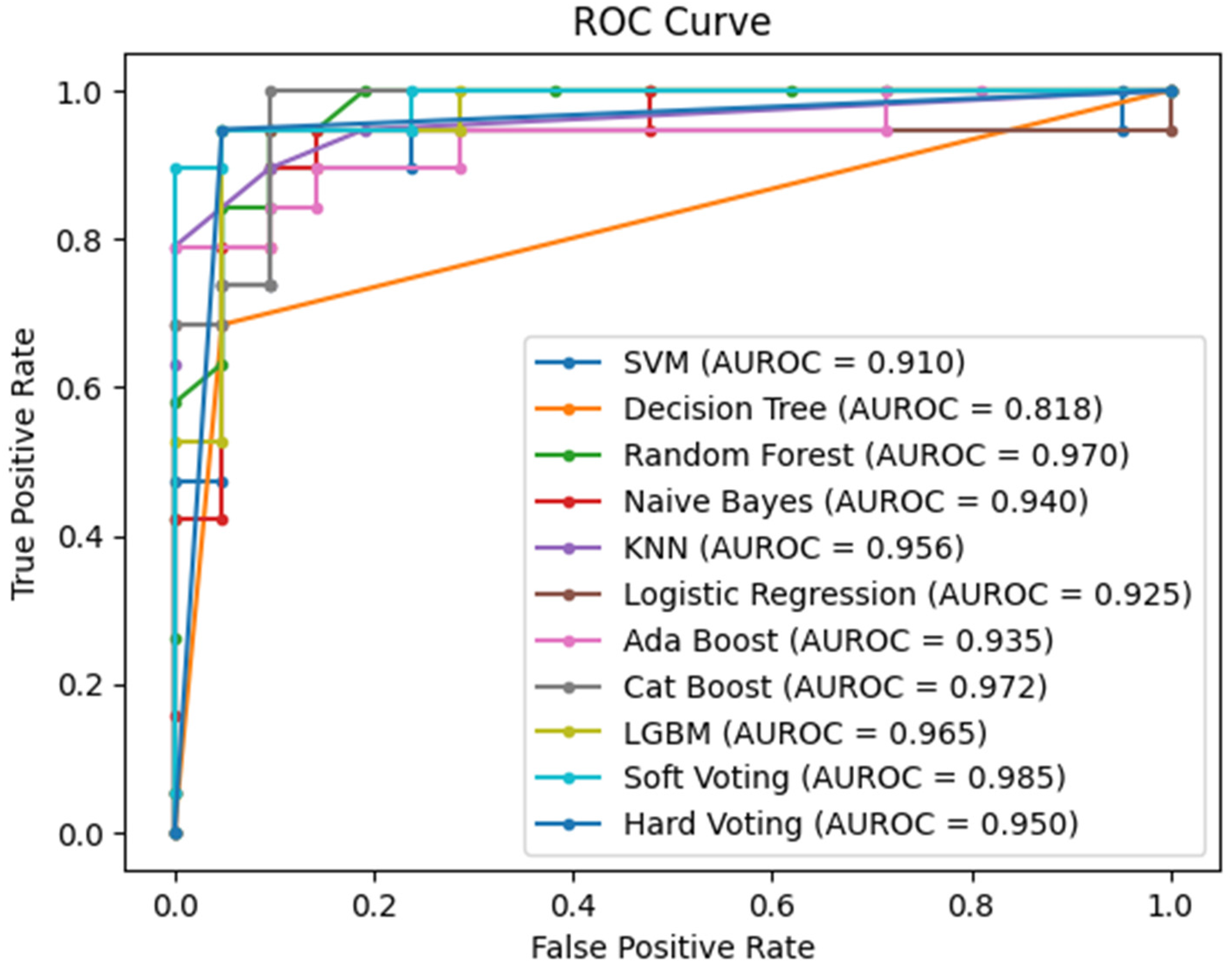
ROC curve of different classifiers.

Overall, 20% dataset was allocated for testing and 80% for training. Table 4 presents the calculations for accuracy, precision, recall, and F1-score. Among the 9 ML classifiers, the SVM classifier and LR performed the best, achieving a maximum accuracy of 92.5%, with 90% precision, 95% recall, and a 92% F1-score for both. Subsequently, a voting classifier was implemented, combining the most accurate classifiers SVM and LR. Using soft voting, the classifier achieved a maximum accuracy of 92.5%, with a precision of 90%, recall of 95%, and an F1-score of 92%.

Table 4.

Measures of the ML model's performance throughout the whole dataset.

ML Algorithms	Accuracy	Precision	Recall	F1-score
Support Vector Machines	92.50%	90%	95%	92%
Decision Tree Classifier	90.00%	94%	84%	89%
Random Forest Classifier	87.50%	89%	84%	86%
Naïve Bayes Classifier	72.50%	90%	47%	62%
KNN Classifier	90.00%	89%	89%	89%
Logistic Regression	92.50%	90%	95%	92%
Ada Boost Classifier	90.00%	100%	79%	88%
Cat Boost Classifier	85.00%	88%	79%	83%
LGBM Classifier	90.00%	88%	79%	83%
Soft Voting Classifier	92.50%	90%	95%	92%
Hard Voting Classifier	95.00%	95%	95%	95%

However, the highest performance was observed with hard voting, where the classifier attained an accuracy of 95%, with 95% precision, 95% recall, and a 95% F1-score. Overall, the hard voting classifier showed the highest performance in terms of accuracy and other metrics, while the Gaussian Naïve Bayes classifier had the lowest accuracy at 72.50%. Figure 7 illustrates the accuracy comparison across different classifiers, including both soft and hard voting classifiers.

Figure 7.

Overall classification accuracy percentages.

Table 4 presents a comparative analysis of the performance of several ML algorithms using four key metrics: F1-score, recall, precision, and accuracy. Among the algorithms, the Hard Voting Classifier stood out, achieving the highest accuracy of 95%, along with balanced performance across precision, recall, and F1-score, each at 95%. This demonstrates its greater capacity to accurately identify both positive and negative cases. The SVM and LR models followed closely with 92.5% accuracy, 90% precision, 95% recall, and an F1-score of 92%, showing strong performance with minimal errors in both false positives and false negatives.

The DT Classifier achieved 90% accuracy with high precision (94%) but lower recall (84%), indicating it missed some true positives. Similarly, the Random Forest Classifier had 87.5% accuracy with a slight imbalance between precision (89%) and recall (84%). The Naïve Bayes Classifier performed the worst, with 72.5% accuracy and low recall (47%) despite high precision (90%). KNN showed a balanced performance with 90% accuracy and 89% across all metrics. The AdaBoost Classifier achieved 90% accuracy and perfect precision (100%), though its recall was lower (79%). Both CatBoost and LGBM classifiers had 85% accuracy, with slightly higher precision (88%) and lower recall (79%). The Soft Voting Classifier matched SVM and Logistic Regression with 92.5% accuracy, 90% precision, and 95% recall, while the Hard Voting Classifier outperformed all with 95% accuracy and balanced metrics across the board.

Interpretability

Figure 8 shows how certain features influence the model's prediction, shifting it from the “base” value (1.437) to the final predicted value (2.00) for a particular instance. The base value represents the average prediction of the model across the entire training set. The higher value of 2.00 suggests that the model predicts the patient is dead from HBV, influenced by the contribution of multiple features. Features in red, such as Varices (0.5517), Protime (0.1789), Spleen Palpable (0.6643), and Ascites (0.6783), push the prediction higher, indicating that they contribute positively to the likelihood of the outcome. Bilirubin (−0.9481) contributes negatively but still raises the overall prediction because it's part of the features pushing the value higher. Albumin (0.9385) is another important feature that raises the prediction. On the other hand, features in blue, such as Spiders (−1.033) and Sgot (−0.7751), decrease the model's prediction, suggesting these features lower the likelihood of the condition.

Figure 8.

SHAP predictions generated using hard voting.

The color red indicates features that push the prediction higher, whereas blue shows features that lower the prediction. This breakdown shows how each feature contributes to the final prediction, explaining the model's decision-making process for this specific instance.

In Figure 9, the SHAP summary plot provides a clear interpretation of how different clinical and demographic features influenced the hard-voting classifier, which combined SVM and LR, in diagnosing HBV. In this case, the SHAP plot reveals that certain features, such as “Albumin,” “Bilirubin,” “Sgot,” and “Age,” played a particularly significant role in determining the final prediction. These features had the highest SHAP values, indicating that they had a strong influence on the model's output. The plot also provides information about the interactions between features. By examining the clustering of dots on the x-axis, it is possible to see how different features interacted with each other to influence the prediction. For example, when two features have dots clustered together to the right of the plot, it suggests that they had a positive interaction, meaning that the combined effect of these features on the prediction was greater than their individual effects.

Figure 9.

Summary plot of the predictions.

Furthermore, the SHAP plot allowed the assessment of the global importance of each feature. By observing the overall position of the dots for a particular feature on the y-axis, one could determine whether it was consistently important across different predictions. Features with dots that were consistently high or low across the plot were considered globally important.

The LIME explanation plot offers a detailed view of how different features influence the hard-voting classifier for a specific prediction of diagnosis for HBV. In Figure 10, Ascites with values between −0.84 and 0.68 has the strongest positive influence on the model's prediction. This means that higher levels of ascites significantly increase the likelihood of a positive HBV diagnosis, reflecting the clinical relevance of fluid accumulation in the abdomen. Albumin, when greater than 0.61, also contributes positively to the prediction, suggesting that elevated albumin levels play a role in supporting a positive diagnosis in this particular case.

Figure 10.

Summary plot of the predictions.

In contrast, Sex with values less than or equal to −0.25, negatively impacts the prediction, indicating that for this instance, the patient's sex decreases the probability of HBV being diagnosed. Bilirubin, which is less than or equal to −0.81, surprisingly has a negative influence, where lower bilirubin levels reduce the likelihood of a positive diagnosis, even though bilirubin is generally a marker of liver dysfunction. Spiders (spider nevi), with values less than or equal to −1.03, also decrease the likelihood of an HBV diagnosis, suggesting that in this local interpretation, the presence of spider nevi steers the model toward a negative result.

On the other hand, the feature Spleen Palpable, with values less than or equal to −0.98, strongly contributes to a positive HBV diagnosis, likely due to its association with advanced liver disease. Anorexia, with a range of −0.61 to 0.66, slightly increases the likelihood of a positive diagnosis, while Malaise, ranging from −0.31 to 1.10, negatively influences the prediction, particularly at higher values. Other features such as Varices (0.21 to 0.55), Sgot (−0.62), and Fatigue (−0.60) have smaller impacts, either positively or negatively, influencing the prediction to a lesser extent.

This LIME explanation provides a transparent, instance-based understanding of how specific features and their values contribute to the classifier's decision, offering clear insights into the factors driving each individual prediction in the outcome of HBV infection.

Discussion

This study demonstrates that ML models can effectively predict mortality risk in HBV-infected patients, with the ensemble Voting Classifier (SVM + LR) achieving the highest accuracy of 95%. Feature selection using the Chi-squared test improved model efficiency, while SMOTE balancing addressed class imbalance, ensuring fairer predictions. Unlike prior studies, this approach integrates both feature selection and data balancing techniques, resulting in a more reliable and interpretable model. The validity of the results is supported by robust performance metrics, including high precision, recall, and F1-score, demonstrating the model's ability to generalize effectively. Model interpretability techniques, including SHAP and LIME, provided insights into the most influential clinical features, such as bilirubin levels and liver enzyme activity. These explainability methods confirmed the importance of key features, reinforcing the clinical relevance of the findings. The superior performance of the approach, compared to previous ML models, highlights its potential as an accurate and interpretable framework for HBV infection. By leveraging advanced ML techniques, this study provides a valuable tool for early HBV prognosis, potentially aiding clinicians in making informed treatment decisions and improving patient outcomes.

Table 5 represents the proposed model's clear superiority when compared to previous studies in terms of accuracy, applied feature selection, and model explainability. With an accuracy of 95.00%, it ranks among the top-performing models, closely matching Fahad R. Albogamy et al. (95.08%)⁸ and V. K. Yarasuri et al. (96.15%).⁵ Although the proposed model slightly trails Fahad R. Albogamy et al. and V. K. Yarasuri et al. in terms of accuracy, it is superior due to its use of feature selection and model explainability, which their models lack. These aspects make the model more efficient, reduce the risk of overfitting, and provide transparency, allowing healthcare professionals to better understand and trust the predictions. The proposed model surpasses others like Shipeng Chen et al. (90.00%)⁹ and V. M. Putri et al. (82.19%).⁶ Many of these models, while achieving high accuracy, such as A. Alamsyah et al. (93.55%)⁷ and Junfeng Peng et al. (91.90%),¹⁰ do not include feature selection or model explainability. In contrast, the proposed model incorporates feature selection, optimizing its focus on the most relevant attributes and improving its overall efficiency and accuracy by reducing potential noise or irrelevant data. Moreover, the proposed model provides model explainability, which is a key differentiator. Most other models, such as Tian et al. (89.1% AUC)³ and V. K. Yarasuri et al., did not offer any explainability, operating more like “black boxes.” Only G. Obaido et al. (92.00%)⁴ included model explainability, but it lacked the feature selection component, which is a crucial factor in refining predictive models. By combining both feature selection and explainability, the proposed model achieves not only high predictive power but also transparency in how decisions are made—an essential attribute in healthcare contexts where understanding model outputs is critical for patient trust and decision-making. This makes the proposed model more robust, interpretable, and ultimately more practical for real-world applications compared to others.

Table 5.

Comparison of the proposed model's performance with previous studies.

Reference	Accuracy	Applied feature selection	Model explainability
Tian et al.³	89.1% (AUC)	No	No
G. Obaido et al.⁴	92.00%	No	Yes
V. K. Yarasuri et al.⁵	96.15%	No	No
V. M. Putri et al.⁶	82.19%	No	No
A. Alamsyah et al.⁷	93.55%	No	No
Fahad R. Albogamy et al.⁸	95.08%	No	No
Shipeng Chen et al.⁹	90.00%	No	No
Junfeng Peng et al.¹⁰	91.90%	No	No
Proposed model	95.00%	Yes	Yes

Strengths

This study has several strengths, including the use of an ensemble Voting Classifier (SVM + LR), which achieved 95% accuracy, surpassing previous models for HBV prognosis. The integration of Chi-squared feature selection enhanced model efficiency by eliminating irrelevant features, while SMOTE balancing effectively addressed class imbalance, ensuring fairer predictions. Additionally, SHAP and LIME provided model interpretability, allowing for clinically relevant insights into the most influential features, making the model more transparent and trustworthy. This holistic approach, balancing high predictive accuracy with model interpretability, makes the study particularly valuable for real-world healthcare applications. Unlike traditional black-box models, our approach ensures that decision-making is explainable, a crucial factor in clinical settings where trust and understanding of predictions are essential.

Limitations

However, this study has some limitations. The dataset used is relatively small (155 patients from the UCI repository), which may impact the model's generalizability to larger and more diverse populations. Despite the application of SMOTE for data balancing, the limited sample size could influence the robustness of the results in real-world settings. Additionally, the dataset lacks certain clinical parameters that might be present in hospital-grade medical records. Future work will involve validating the model on larger, real-world datasets across different demographics and regions to enhance its applicability. Furthermore, exploring additional ML techniques and deep learning approaches could further improve predictive performance while maintaining interpretability.

Moreover, the inclusion of specific clinical features such as splenomegaly and varices, which are well-established indicators of cirrhosis, may introduce inherent clinical bias into the model. These features often signify a more advanced stage of chronic Hepatitis B infection and are strongly correlated with increased mortality due to complications like portal hypertension and liver failure. As a result, the model may place disproportionate weight on these late-stage features when learning predictive patterns, potentially leading to an overestimation of mortality risk in patients presenting with such conditions. This bias could compromise the model's ability to generalize across the full clinical spectrum, particularly in identifying early-stage patients who may not exhibit these severe symptoms. Furthermore, given the relatively small and imbalanced nature of the dataset, such influential features might dominate the learning process, resulting in reduced sensitivity to more subtle, early-stage indicators. To address this limitation, future work will involve a more granular analysis of feature contributions across disease stages. Specifically, we plan to stratify the patient cohort based on clinical severity (e.g., cirrhotic vs. non-cirrhotic) and evaluate model performance within each subgroup to assess differential predictive behavior. We also intend to explore ablation studies by removing high-risk cirrhosis-related features (e.g., varices, splenomegaly) to evaluate the model's reliance on them and its ability to generalize without such markers. Additionally, incorporating larger and more diverse clinical datasets—including early-stage and asymptomatic HBV cases—will be a priority to enhance the robustness and applicability of the model. By doing so, we aim to build a more balanced and clinically comprehensive predictive framework that supports risk assessment across the full continuum of Hepatitis B disease progression.

Conclusions

This study integrates sophisticated classifiers and feature selection techniques to apply machine learning (ML) techniques to the detection of Hepatitis B virus (HBV). A voting classifier that combined logistic regression (LR) and support vector machines (SVM) outperformed standalone models, achieving 95% accuracy. By correcting for class imbalance, chi-squared feature selection and the Synthetic Minority Over-sampling Technique (SMOTE) enhanced performance. SHAP and LIME were used to improve interpretability, offering important insights into noteworthy characteristics such as high bilirubin levels. This guarantees clear and reliable forecasts, which makes the model helpful for medical practitioners. The tiny dataset (155 patients) is a significant restriction that could limit generalizability. Testing on bigger, more varied datasets are required to confirm efficacy across various populations, even when SMOTE is used for balancing. This research provides a dependable and interpretable approach for HBV diagnosis by striking a balance between high predictive accuracy and model explainability. Integrating SHAP and LIME guarantees transparent decision-making, which is essential in the healthcare industry and is not possible with black-box models. Testing with bigger datasets should be the main goal of future research in order to improve the model's clinical usefulness and resilience.

Footnotes

ORCID iD

Khandaker Mohammad Mohi Uddin

Ethical considerations

Not required

Consent to participate

Not required

Author contributions

Abid Bin Ahosan: conceptualization, methodology, and software; Forhadul Islam: resources, formal analysis, and writing—original draft; Mr Nahid Hasan: validation and visualization; Khandaker Mohammad Mohi Uddin: supervision, validation, methodology, and writing—original draft, Md Ashraf Uddin: writing—review and editing and supervision.

Funding

The authors received no financial support for the research, authorship, and/or publication of this article.

Declaration of conflicting interests

The authors declared no potential conflicts of interest with respect to the research, authorship, and/or publication of this article.

Data availability statement

The data supporting this study's findings are available from the corresponding author upon reasonable request.

References

Tan

Bhadoria

. Estimating the proportion of people with chronic hepatitis B virus infection eligible for hepatitis B antiviral treatment worldwide: a systematic review and meta-analysis. Lancet Gastroenterol Hepatol 2021; 6: 106–119.

Breakwell

Marke

. Assessing the impact of the routine childhood hepatitis B immunization program and the need for hepatitis B vaccine birth dose in Sierra Leone. Vaccine 2022; 40: 2741–2748.

Tian

Chong

Huang

, et al. Using machine learning algorithms to predict hepatitis B surface antigen seroclearance. Comput Math Methods Med 2019; 2019: 6915850.

Obaido

Ogbuokiri

Swart

, et al. An interpretable machine learning approach for hepatitis B diagnosis. Appl Sci 2022; 12: 11127.

Yarasuri

Indukuri

Nair

. Prediction of hepatitis disease using machine learning technique. In: 2019 Third International conference on I-SMAC (IoT in Social, Mobile, Analytics and Cloud) (I-SMAC), Palladam, India, 2019, pp.265–269.

Putri

Masjkur

Suhaeni

. Performance of SMOTEinarandomforestandnaiveBayesclassifierforimbalanced Hepatitis-B vaccination status. J Physics: Conf Ser 2021; 1863: 012073.

Alamsyah

. Increased accuracy of prediction hepatitis disease using the application of principal component analysis on a support vector machine. J Phys: Conf Ser 2021; 1968: 012016.

Albogamy

Asghar

Subhan

. Decision Support System for Predicting Survivability of Hepatitis Patients. Front Public Health 2022; 10: 1–15.

Chen

. Using Quasispecies Patterns of Hepatitis B Virus to Predict Hepatocellular Carcinoma With Deep Sequencing and Machine Learning. J Infect Dis 2021; 223: 1887–1896.

10.

Peng

. An Explainable Artificial Intelligence Framework for the Deterioration Risk Prediction of Hepatitis Patients. J Med Syst 2021; 45: 61.

11.

University of California Irvine (UCI) Machine Learning Repository | Hepatitis B dataset.

12.

Chawla

. SMOTE: Synthetic Minority Over-sampling Technique. J Artif Intell Res 2002; 16: 321–357.

13.

Ali

PJM

. Data Normalization and Standardization: A Technical Report, January 2014.

14.

Qin

Chen

Liu

, et al. A machine learning methodology for diagnosing chronic kidney disease. IEEE Access 2020; 8: 20991–21002.

15.

Mindrila

Balentyne

. The Chi Square Test, Based on Chapter 23 of The Basic Practice of Statistics (6th ed.).

16.

Ana

Morelato

Roux

, et al. Review of the most common chemometric techniques in illicit drug profiling. Forensic Sci Int 2019; 302: 109911.

17.

Walker

Duncan

. Estimation of the probability of an event as a function of several independent variables. Biometrika 1967; 54: 167–179.

18.

Zhang

, et al. Novel binary logistic regression model based on feature transformation of XGBoost for type 2 diabetes Mellitus prediction in healthcare systems. Future Gener Comput Syst 2022; 129: 1–12.

19.

Ogbuokiri

Ahmadi

Nia

, et al. Vaccine Hesitancy Hotspots in Africa: An Insight from Geotagged Twitter Posts. IEEE Trans Comput Soc Syst 2023; 11: 1325–1338.

20.

Mienye

Obaido

Aruleba

, et al. Enhanced prediction of chronic kidney disease using feature selection and boosted classifiers. In: International Conference on Intelligent Systems Design and Applications, 2022, pp.527–537. Cham, Switzerland: Springer.

21.

Schlkopf

Smola

. Learning with Kernels: Support Vector Machines, Regularization, Optimization, and Beyond (Adaptive Computation and Machine Learning. Cambridge: MIT Press, 2001.

22.

Huang

Chen

Lin

, et al. SVM And SVM ensembles in breast cancer prediction. PLoS ONE 2017; 12: e0161501.

23.

Ghosh

Sanyal

. An ensemble approach to stabilize the features for multi-domain sentiment analysis using supervised machine learning. J Big Data 2018; 5: 1–25.

24.

Mahabub

Mahmud

Hossain

. A robust system for message filtering using an ensemble machine learning supervised approach. ICIC Expr Lett Part B Appl 2019; 10: 805–811.

25.

Zhao

Lee

Jeong

S-P

. Decision tree application to classification problems with boosting algorithm. Electronics (Basel) 2021; 10: 1903.

26.

Breiman

Friedman

Olshen

, et al. Classification and Regression Trees. London, UK: Routledge, 2017.

27.

Quinlan

. Induction of decision trees. Mach Learn 1986; 1: 81–106.

28.

Quinlan

. C4. 5: Programs for Machine Learning. Amsterdam, The Netherlands: Elsevier, 2014.

29.

Mienye

Sun

Wang

. An improved ensemble learning approach for the prediction of heart disease risk. Inform. Med Unlocked 2020; 20: 100402.

30.

Schonlau

Zou

. The random forest algorithm for statistical learning. Stata J 2020; 20: 3–29.

31.

Lin

, et al. An ensemble random forest algorithm for insurance big data analysis. IEEE Access 2017; 5: 16568–16575.

32.

Tomar

Verma

Jha

. Web page classification using modified naïve baysian approach. In: IEEE TENCON-2006, 14-17 Nov 2006, pp.1–4.

33.

Linero

Antonelli

. The how and why of Bayesian nonparametric causal inference. Wiley Interdisciplinary Reviews: Comput Stat 2023; 15: e1583.

34.

Sameer

Gupta

. CNN based framework for detection of epileptic seizures. Multimed Tools Appl 2022; 81: 17057–17070.

35.

Meng

Finley

, et al. LightGBM: A Highly Efficient Gradient Boosting Decision Tree.

36.

Caruana

Niculescu-Mizil

. An empirical comparison of supervised learning algorithms. In: Proceedings of the 23rd International Conference on Machine Learning, Pittsburgh, PA, USA, 25–29 June 2006, pp.161–168.

37.

Sevinç

. An empowered AdaBoost algorithm implementation: a COVID-19 dataset study. Comput Ind Eng 2022; 165: 107912.

38.

Lee

Tseng

Yang

, et al. Random RotBoost: an ensemble classification method based on rotation forest and AdaBoost in random subsets and its application to clinical decision support. Entropy 2022; 24: 617.

39.

Zheng

Xiao

Sun

, et al. Brillouin frequency shift extraction based on AdaBoost algorithm. Sensors 2022; 22: 3354.

40.

Huang

Jin

, et al. Fair-AdaBoost: extending AdaBoost method to achieve fair classification. Expert Syst Appl 2022; 202: 117240.

41.

Ding

Zhu

Chen

, et al. An efficient AdaBoost algorithm with the multiple thresholds classification. Appl Sci|3192 2022; 12: 5872.

42.

Mangalathu

Hwang

Jeon

. Failure mode and effects analysis of RC members based on machine-learning-based SHapley additive exPlanations (SHAP) approach. Eng Struct 2020; 219: 110927.

43.

García

Aznarte

. Shapley additive explanations for NO2 forecasting. Ecol Inform 2020; 56: 101039.

44.

Santos

Yamouni

Albiero

, et al. Gradient boosting and shapley additive explanations for fraud detection in electricity distribution grids. Int Trans Electr Energy Syst 2021; 31: e13046.

45.

Meddage

Ekanayake

Perera

, et al. Interpretation of machine-LearningBased (black-box) wind pressure predictions for low-rise gable-roofed buildings using shapley additive explanations (SHAP). Buildings 2022,; 12: 34.

46.

Rao

Mehta

. A Study of LIME and SHAP Model Explainers for Autonomous Disease Predictions, 2022.

47.

Rainio

Teuho

Klén

. Evaluation metrics and statistical tests for machine learning. Sci Rep 2024; 14: 6086.

Improving Hepatitis B outcome prediction with ensemble machine learning: A study on predictive models and interpretability

Abstract

Objective

Methods

Results

Conclusion

Keywords

Introduction

Materials and methods

Dataset preparation

Features selection

Machine learning models

Logistic regression

Support vector machine

Voting classifier

Other used ML models

Model explainability techniques

SHapley Additive exPlanations (SHAP)

Local Interpretable Model-agnostic Explanations (LIME)

Environmental setup

Performance matrix

Results

Performance analysis

Interpretability

Discussion

Strengths

Limitations

Conclusions

Footnotes

ORCID iD

Ethical considerations

Consent to participate

Author contributions

Funding

Declaration of conflicting interests

Data availability statement

References