
Abstract
Objective
To improve the accuracy and explainability of skin lesion detection and classification, particularly for several types of skin cancers, through a novel approach based on the convolutional neural networks with attention-integrated customized ResNet variants (CRVs) and an optimized ensemble learning (EL) strategy.
Methods
Our approach utilizes all ResNet variants combined with three attention mechanisms: channel attention, soft attention, and squeeze-excitation attention. These attention-integrated ResNet variants are aggregated through a unique multi-level EL strategy. We propose an innovative weight optimization method, inverse Gini indexed averaging (IGIA), which is further extended to multi-leveled IGIA (ML-IGIA) to determine the optimal weights for each model within multiple ensemble levels. For interpretability, we employ gradient class activation map to highlight the regions responsible for classification dominance, enhancing the model’s transparency.
Results
Our method was evaluated on the Human Against Machines 10000 dataset, achieving a superior accuracy of 94.52% with the ML-IGIA approach, outperforming existing methods.
Conclusions
The proposed CRV-based ensemble model with ML-IGIA demonstrates robust performance in skin lesion classification, offering both high accuracy and enhanced interpretability. This approach addresses the current research gap in effective weight optimization in EL and supports timely, automated skin disease detection.
Keywords
Introduction
Skin lesions denote irregular alterations in the skin’s appearance, while skin ailments encompass a wide array of issues affecting the skin’s well-being, structure, and operation. These ailments vary widely, spanning from common conditions like acne to more serious concerns such as skin cancer. Skin diseases may present diverse symptoms and are not solely characterized by the presence of lesions. Skin lesions can arise from infections, inflammatory disorders, allergic responses, skin malignancies, insect stings, injuries, autoimmune conditions, hereditary factors, environmental influences, vascular irregularities, warts, and cysts, each with its distinct causes and attributes. Skin lesions can broadly be classified into two categories based on their potential harm: “Non-cancerous skin lesions” are benign and typically pose no threat. Instances include moles, skin tags, warts, seborrheic keratoses, and hemangiomas, while “Cancerous skin lesions” are malignant lesions with the capacity to metastasize to other body parts. The most prevalent types of malignant skin lesions encompass basal cell carcinoma, squamous cell carcinoma, and melanoma.
The combination of clinical evaluations and diagnostic tests is typically essential for effective diagnosis and treatment. Neglecting symptoms can lead to serious consequences, including the development of skin cancer, which is the most prevalent form of cancer globally.
1
A recent study claims, skin diseases and cancers have been reported in children as young as under even 5 months old.
2
Melanoma, though relatively rare, is responsible for the majority of skin cancer-related deaths.
3
There were
The early detection of skin abnormalities holds immense importance. However, many individuals might lack awareness due to the extensive range of medical assessments needed, along with the accompanying financial burdens. A study provides some massive data about skin lesion education among lowa family physicians. 6 Dermatoscopy, also known as dermoscopy or epiluminescence microscopy, is a non-invasive diagnostic method in dermatology that utilizes a specialized handheld device with magnification and lighting to examine skin lesions. 2 This aids in the early identification of skin cancer and other dermatological conditions compared to traditional detection methods. However, this technique heavily relies on expert interpretation, leaving room for human errors.
On the other hand, an artificial intelligence (AI) powered automated system, especially utilizing machine learning (ML), and deep learning (DL) techniques, has the potential to identify skin abnormalities by analyzing a limited dataset of images. Such a system could significantly accelerate early diagnosis, raising awareness about the condition and potentially leading to more effective medical interventions. Numerous researchers are exploring the application of ML and DL techniques. However, there remains ample scope for improvement in this area. One crucial aspect is the effective training of models to reduce reliance on classes with abundant data. Directly applying models based on transfer learning (TL), pre-trained on the ImageNet dataset, may struggle to extract superficial features, making them unsuitable for specific datasets unless carefully adjusted. While some approaches involve integrating different models, determining the optimal contribution of each model can pose challenges and influence overall performance. Furthermore, the current state of models does not prioritize ensuring the interpretability of results. Moreover, utilizing the same data for both validation and testing purposes can introduce bias and impact the accuracy of model assessment.
Previously, numerous researchers have employed convolutional neural networks (CNNs) and ensemble learning (EL) methodologies to mitigate the inherent limitations of individual models. However, their endeavors were hindered by the absence of an optimal weight selection mechanism for each model, thereby impeding the attainment of the most accurate results. Conventional ensemble techniques such as majority voting, softmax averaging (assigning equal weights to each prediction), weighted prediction (utilizing arbitrarily chosen weights), and so on were commonly utilized. Nonetheless, these methods failed to account for the varying significance of individual predictions, as certain models might have gleaned more valuable insights during training. This inherent oversight underscores the limitations of prior research in this domain.
In this study, we address class imbalance by systematically augmenting the training dataset, ensuring each class is represented proportionally. This balanced distribution minimizes bias, enhancing the model’s reliability across test and validation phases. We further enhance feature focus by implementing three tailored attention mechanisms—channel attention (CA), soft attention (SA), and squeeze-excitation attention (SEA)—across ResNet variants. This strategic use of attention layers improves the model’s sensitivity to critical features in the input data. Our novel EL approach, termed inverse Gini indexed averaging (IGIA), introduces a more efficient and precise method for weighting the ResNet variants within the ensemble. Unlike conventional brute-force approaches, IGIA assigns optimal model weights based on the inverse Gini index, boosting the architecture’s overall accuracy and stability. Additionally, we prioritize model interpretability by integrating gradient class activation maps (GradCAMs) visualization, enabling the model to highlight specific areas relevant to diagnosing skin conditions and thereby providing deeper insights into its decision-making process.
In this research, our approach is carefully crafted to directly tackle these constraints. Additionally, the primary aim revolves around addressing the core research queries outlined below, with the development of a sturdy architectural framework based on furnishing appropriate responses to them. These research questions are essential, requiring thorough responses.
RQ1: What measures can be taken to attain an even distribution of classes in the multi-class dataset?
Since there can be discrepancies in the number of samples across classes, there’s a risk of overrepresentation from majority classes, which could impede the precise prediction of minority classes. Therefore, ensuring a balanced distribution of classes is imperative.
RQ2: How can we employ a method to emphasize the most crucial attributes, particularly focusing on vital areas or zones?
Certain parts of an image might not contribute significantly to feature extraction in a classification scenario because of redundant or irrelevant data that could have adverse effects, while others may play a more substantial role in indicating the target class.
RQ3: Does relying solely on one model suffice, or is there a necessity for supplementary EL techniques, and if yes, which one should be utilized?
It is known that not every model can proficiently classify all types of data, so it’s crucial to reduce dependence on a single model. Therefore, an EL technique could be the most appropriate resolution.
RQ4: What are the constraints of conventional EL methods that justify the introduction of a novel EL approach?
Since no method can guarantee the precise allocation of the optimal ratio for each model’s prediction, it’s essential to introduce a novel approach capable of computing the optimal ratio of predictions for ensemble models. We effectively address the challenge of class imbalance by rigorously augmenting the training dataset. This strategic augmentation is carried out while ensuring a balanced distribution across classes, thereby preventing any bias towards dominant classes in the model. Consequently, our architecture demonstrates reliability and impartiality in the evaluation of test and validation data. To ensure adequate focus on crucial features, we ingeniously incorporate three attention mechanisms, CA, SA, and SEA, within individually tailored ResNets architectures. This innovative approach enables models to concentrate on the most significant aspects of the input data. We present a novel EL approach termed IGIA, which aims to determine optimal weights for each ResNet variant involved in the ensemble. Unlike traditional brute-force methods for assigning weights to multiple models, IGIA offers a more efficient and effective solution. This innovative technique operates across multiple levels, strategically enhancing the performance of the architecture. To prioritize the interpretability of the model, we GradCAM visualization. This advanced visualization technique allows the model to pinpoint specific regions relevant to diagnosed skin conditions, thereby enhancing the transparency and insightfulness of the architecture.
In response to the aforementioned inquiries, we formulate our research methodology to not only mitigate the constraints observed in prior studies but also to provide comprehensive insights into the specified research questions. This approach is aimed at offering the following contributions:
The arrangement of the article is meticulously structured to ensure clarity and coherence. It begins with an extensive exploration of the existing literature in the “Literature review”sec section, followed by a detailed presentation of the materials and methods in the “Dataset description”sec and “Research methodology”sec sections. The subsequent section, the “Experimental results analysis”sec section, offers a succinct yet comprehensive analysis of the achieved performances. Expanding on these findings, the “Discussion and extended comparison”sec section delves into a thorough discussion, evaluating the model’s practical implications. The limitations of the study are carefully delineated in the “Threats to validity”sec section, providing a comprehensive perspective. Ultimately, the “Conclusion and Future Work”sec section wraps up the article, summarizing the key insights and contributions of the study.
Literature review
The realm of skin lesion classification has been thoroughly explored by numerous researchers, who have dedicated their efforts to unraveling the intricate complexities within this field. In this section, we embark on a journey to illuminate the diverse contributions as well as limitations of these studies. Studies from Shafin et al., 7 Efat et al., 8 and Nivedha and Shankar 9 demonstrated different types of lesions with novel classification strategies while from Ren, 10 Maqsood et al., 11 and Hussain et al. 12 provided several customized models to classify skin lesion properly. From the endeavors Khan et al., 13 Bibi et al., 14 and Shetty et al., 15 a custom CNN architecture was utilized, while Sevli, 16 Saarela and Geogieva, 17 and Nie et al. 18 incorporated various transformation processes. In contrast, the studies of Hoang et al., 19 Sun et al., 20 Mahbod et al., 21 Rahman et al., 22 Wang et al., 23 Harangi et al., 24 Khan et al., 25 and Popescu et al. 26 concentrated on feature extraction through TL, while Gouda et al. 27 and Nigar et al. 28 employed soft attention in conjunction with TL.
Nivedha and Shankar 9 proposed a melanoma diagnosis framework combining faster region CNNs (Faster R-CNNs) with the African Gorilla Troops Optimizer (AGTO) algorithm for feature selection. The methodology reduces analytic complexity by optimizing feature selection with AGTO and employs Faster R-CNN for classification, achieving 98.55% accuracy on the ISIC-2020 dataset. While the framework outperforms four existing models, it lacks a dedicated method to identify optimal image regions. Ren 10 proposed a monkeypox detection approach utilizing twelve pretrained CNN models, including DenseNet201, efficientNet variants, and InceptionV3, to address limited sample availability. The study achieved the highest performance with DenseNet201, reporting 98.89% accuracy for binary classification, 100% for four-class classification, and 99.94% for six-class classification. Despite these results, the direct use of pretrained models without fine-tuning limits their adaptability to specific skin dataset. Maqsood and Damaševičius 11 proposed a deep learning-based framework for skin lesion localization and classification, incorporating bio-inspired contrast enhancement and a custom 26-layer CNN for lesion segmentation. Pre-trained models (Xception, ResNet-50, ResNet-101, and VGG16) were fine-tuned, and their feature vectors were fused using convolutional sparse image decomposition, followed by feature selection via a Poisson distribution method and classification with a multi-class SVM. The model achieved notable accuracies of 98.57% on HAM10000, 98.62% on ISIC2018, 93.47% on ISIC2019, and 98.98% on PH2 datasets, surpassing state-of-the-art methods, though it lacked specific region selection and dataset balancing.
Hussain et al. 12 introduced a deep learning-based framework for multiclass skin lesion classification, incorporating contrast enhancement using dark channel haze and top-bottom filtering. The methodology involved fine-tuning pre-trained models through genetic algorithm-based hyperparameter optimization, feature fusion using a serial correlation approach, and feature selection via an improved anti-Lion optimization algorithm. The framework achieved remarkable accuracy of 96.1% on ISIC2018 and 99.9% on ISIC2019 datasets, outperforming existing techniques. Their limitation existed in specifying the most important region with better explainability. Khan et al. 13 proposed an innovative architecture combining deep learning with entropy-NDOELM for multiclass classification of skin lesions, overcoming challenges related to accuracy and computational cost. The approach incorporates contrast enhancement, optimization of EfficientNetB0 and DarkNet19 models, feature extraction and selection using entropy-NDOELM, feature fusion, and classification through an extreme learning machine, achieving over 90% accuracy across all datasets. Bibi et al. 14 developed MSRNet, a deep learning-based framework for multiclass skin lesion recognition, incorporating contrast enhancement using image luminance information. The methodology involved fine-tuning DarkNet-53 and DenseNet-201 with additional residual blocks, hyperparameter optimization via a genetic algorithm, feature fusion using a serial-harmonic mean approach, and feature selection through marine predator optimization controlled by Rényi entropy. The framework achieved accuracies of 85.4% on ISIC2018 and 98.80% on ISIC2019 datasets, outperforming recent techniques, though the dataset imbalance was noted as a limitation.
In a study by Shetty et al., 15 a CNN was utilized for skin cancer detection, achieving an accuracy rate of 94%. However, their method was limited by using only a subset of the dataset (200 images per class), which was then augmented, raising concerns about the applicability of the results to the entire dataset. Sevli 16 developed a CNN model for skin lesion classification, integrating it with a web application via a REST API. The model underwent evaluation by dermatologists in two phases, achieving an accuracy of 91.51%. Notably, their customized CNN design was unable to focus on critical features. In a different approach, Saarela and Geogieva 17 introduced a novel method based on the Bayesian inference to improve model interpretability, demonstrating its effectiveness. However, their achieved accuracy of 80% on the test data falls short of being particularly promising.
Nie et al. 18 proposed a hybrid CNN transformer model enhanced with focal loss for skin lesion classification, achieving an accuracy of 89.48%. Their approach combined a CNN for extracting low-level features and a vision transformer, although there is a limitation in extracting deep features. Hoang et al. 19 introduced an innovative segmentation technique and utilized the lightweight neural network architecture, wide-ShuffleNet, for skin lesion classification, resulting in comparatively lower accuracy. Their achieved accuracies were 84.80% and 86.33% on different sizes of test data. In another study by Sun et al., 20 a model was proposed that incorporated additional metadata and integrated supplementary information during the data augmentation process. The approach yielded an accuracy of 88.7% with a single model and 89.5% for the embedding solution. The augmentation process was not described in a well-interpretable manner.
Mahbod et al. 21 examined the influence of image size on skin lesion classification. Their investigation utilized TL techniques and underscored the efficacy of a multi-CNN fusion approach, achieving a balanced multi-class accuracy of 86.2%, albeit with a comparatively heavy model. Rahman et al. 22 formulated a weighted average EL model that leveraged five deep neural network models via TL. This ensemble method notably improved the outcomes, resulting in an impressive accuracy of 88%. However, the direct utilization of pre-trained models hindered the adaptation of the model to the specific dataset.
Wang et al. 23 introduced a novel two-stream network called the feature fusion module, which intelligently merged DenseNet-121 and VGG-16. This fusion aimed to extract multiscale pathological information using multi-receptive fields and GeM pooling to reduce the spatial dimensionality of lesion features. Despite achieving an elevated test accuracy of 91.24%, there was a deficiency in fine-tuning the pre-trained model. Harangi et al. 24 proposed a TL-based CNN framework for multiclass classification utilizing binary classification outcomes. Their study demonstrated that incorporating binary classification results significantly improved the accuracy, with an average of 93.46% for the multi-class problem, representing a notable increase of 7%. However, their approach of combining binary classification with multi-class lacked justification.
Khan et al. 25 utilized Resnet50 alongside a feature pyramid network for skin lesion segmentation, followed by a 24-layered CNN for classification, resulting in an accuracy of 86.5%. However, their approach omitted the integration of mask information from the classification dataset (Human Against Machines 10000 (HAM10000)) during the segmentation phase. Popescu et al. 26 devised a system for skin lesion classification, employing various TL techniques alongside collective intelligence. Their methodology achieved a validation accuracy of 86.71% through a decision fusion module. Notably, no results were provided for an independent test dataset. Gouda et al. 27 improved the quality of skin lesion images using ESRGAN before applying a CNN, resulting in an accuracy of 83.2%. Despite experimenting with multiple TL models, their study did not address the issue of imbalanced data. Nigar et al. 28 introduced an explainable AI-based skin lesion classification system, leveraging the LIME framework and ResNet-18. This approach achieved notable accuracy (94.47%) and interpretability, aiding in the early-stage skin cancer diagnosis. Limitations include reliance on a single pre-trained model, a small dataset, and potential downsizing effects on image pre-processing.
Nguyen et al. 29 proposed an innovative method that combined DL with SA, obtaining a 90% accuracy using InceptionResNetV2 and an 86% accuracy using MobileNetV3Large. They did not clarify the rationale behind using SA instead of other modules. Datta et al. 30 investigated the impact of the SA mechanism in skin cancer classification, aiming to enhance model performance. Their work surpassed state-of-the-art precision and AUC scores on two datasets, achieving an impressive accuracy of 93.4%. This model holds the potential for assisting dermatologists in dermoscopy systems, although it could not identify appropriate color channel weights for attention.
Taking cues from the insights provided in the previously discussed literature, our research identifies and tackles certain limitations. Primarily, we employ the entire dataset for our investigation, with a specific emphasis on augmenting the training set to address the issue of data imbalance. This guarantees the independence of the test set, enabling a more precise evaluation of the model on unseen data. We pinpoint the crucial regions of interest by utilizing the AT method and integrating it seamlessly with TL models. Moreover, after extracting intricate features, we fine-tune the TL models and customized ResNet variants (CRV) architecture, thereby reducing the dependence on the ImageNet dataset.
Dataset description
This study utilized the publicly available HAM10000 dataset, which was obtained from the Harvard Dataverse repository and is made available under the Attribution-NonCommercial 4.0 International license. The dataset was carefully curated by Tschandl et al. (2018) 31 to provide a comprehensive collection of diverse skin lesion samples. It includes 10,015 dermatoscopic images in jpg format, categorized into seven classes: melanoma (MEL), nevus (NV), vascular lesions (VASC), actinic keratosis (AK), basal cell carcinoma (BCC), benign keratosis (BKL), and dermatofibroma (DF). MEL, AK, and BCC represent the cancerous lesions, whereas NV, BKL, and DF are the non-cancerous lesions. It is important to note that some VASC lesions can also be cancerous. The use of this dataset in this study complies with the terms of the license, which allows for non-commercial use with appropriate attribution. A summary of the dataset’s details is provided in Table 1.
Detailed description of the dataset.

Figure 1 illustrates the examples of images, showcasing one sample per class within the dataset. Additionally, Figure 2 highlights the significant class representation imbalance evident in the dataset’s class distribution.
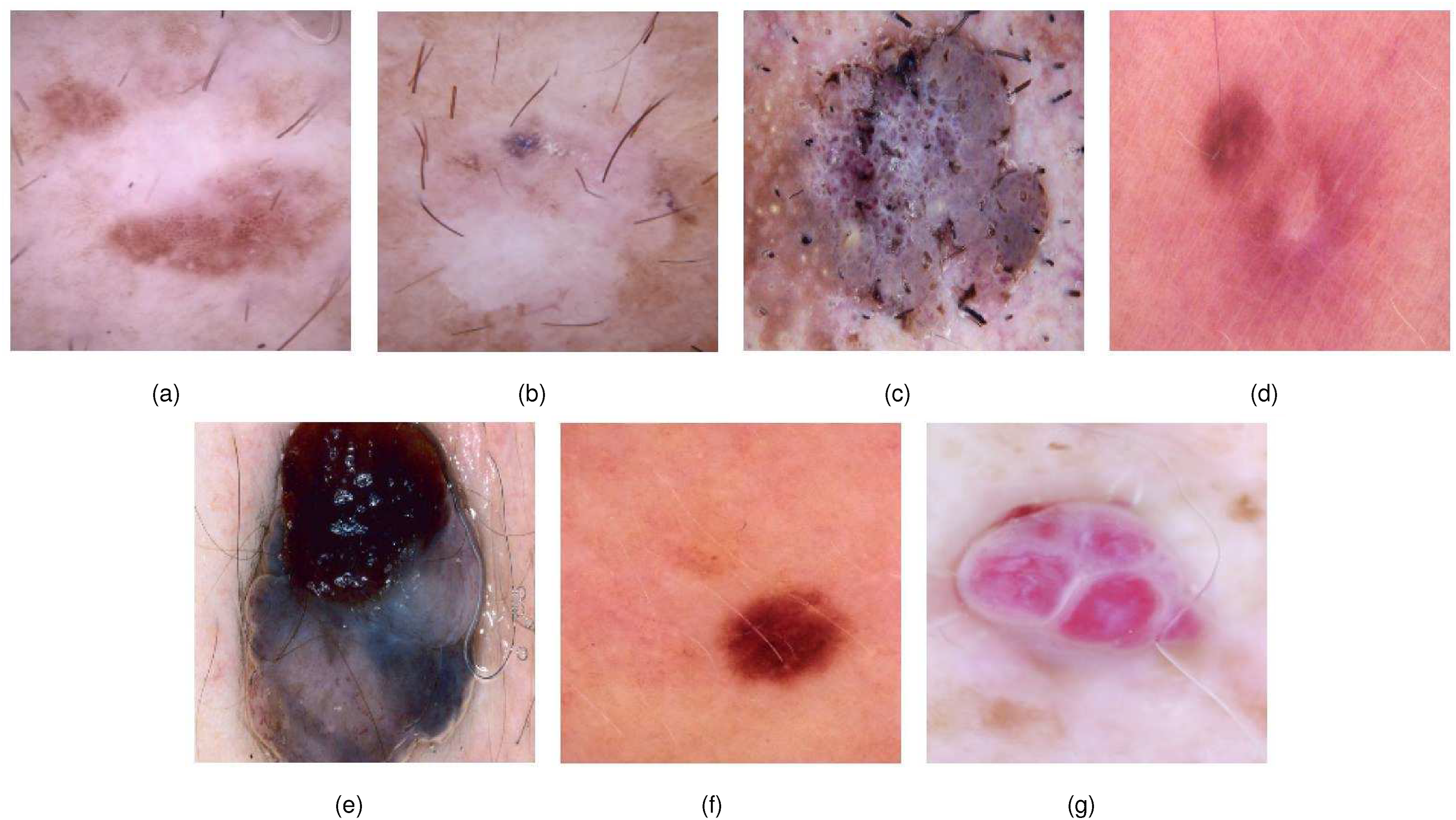
Sample images of each class: (a) actinic keratosis (AK), (b) basal cell carcinoma (BCC), (c) benign keratosis (BKL), (d) dermatofibroma (DF), (e) melanoma (MEL), (f) nevus (NV), and (g) vascular lesions (VASC).

Imbalanced class sample distribution.
Research methodology
Our methodology began with dataset collection, followed by crucial data preprocessing steps. Subsequently, the dataset was partitioned into training, testing, and validation subsets. To address class imbalances, augmentation processes were exclusively applied to the training data, ensuring independent validation on unseen testing and validation data. CRV architectures were deployed and fitted using the training data, with validation conducted on the validation subset. The performance of these fitted models was evaluated using the testing data. Predictions generated by each architecture were aggregated through IGIA to enhance overall performance. The evaluation of IGIA was conducted at multiple levels to validate our approach. In conclusion, the GradCAM visualization technique was utilized to offer visual representations of the crucial regions responsible for predictions. The sequential workflow of this investigation is illustrated in Figure 3.
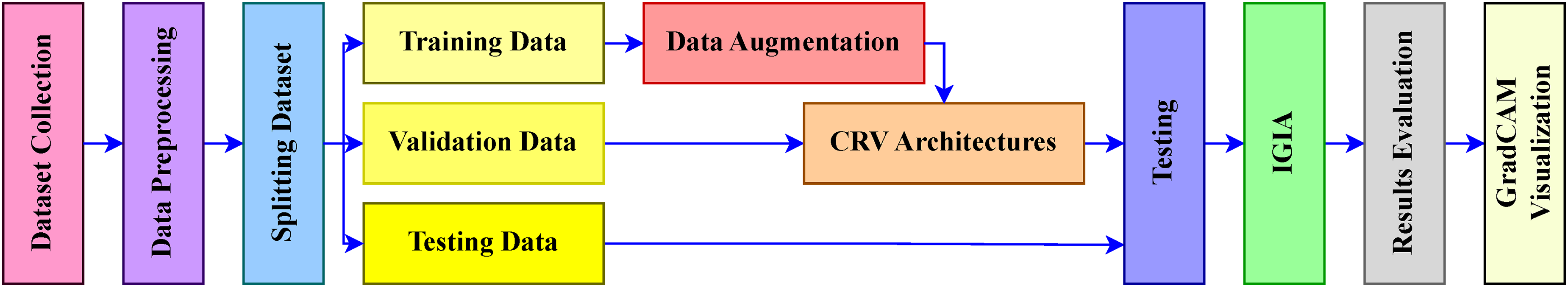
Schematic depiction of methodology.
Data preprocessing and training set augmentation
During this phase, the categorization of images based on their lesion ID was initiated, followed by the specific selection of distinct samples for division into training, testing, and validation sets. To enhance the credibility and resilience of our approach, additional redundant images were introduced to the training dataset, enabling testing with previously unencountered samples. The dataset was partitioned, with 15% reserved for validation and an additional 15% for testing, while the remaining images were designated for training purposes. Augmentation procedures were strictly applied only to the training data to ensure the independence of the test and validation sets. If augmentation had been applied to the test or validation data as well, it might have resulted in duplicate samples appearing in the training, validation, and test sets. Such overlap could compromise the reliability of the model’s evaluation. By limiting augmentation to the training data, the class imbalance problem was addressed while keeping the test and validation sets completely unseen by the model during training. This approach resulted in
In our research, we implemented an advanced image augmentation strategy using TensorFlow’s “ImageDataGenerator,” starting with enhancing the contrast of the original images. This preprocessing step ensured that the images were optimally contrasted before augmentation. Our augmentation process encompassed a variety of transformations to significantly diversify the training data and bolster the model’s robustness. We applied random rotations up to

Sample images of the samples after augmentation: (a) original sample, (b) rotated sample, (c) width_shifted sample, (d) height_shifted sample, (e) zoomed sample, (f) horizontal_flipped sample, and (g) vertical_flipped sample.
Creation of CRV architectures in association with attention mechanisms
Our primary focus centered on utilizing TL-based ResNet variants to effectively harness the principles of pre-trained architectures. This process initiated with the utilization of saved weights from pre-trained models, ensuring precision in our study. To achieve this, we leveraged various variants of pre-trained ResNet models, including ResNet50, ResNet101, ResNet152, ResNetv2 variants such as ResNet50v2, ResNet101v2, and ResNet152v2, and ResNetRS variants like ResNetRS50, ResNetRS101, ResNetRS152, ResNetRS200, ResNetRS270, ResNetRS350, and ResNetRS420. These variants were designed to accept input images of size 224
Given that these weights were not originally trained for our dataset, we undertook the process of fine-tuning them. This fine-tuning was conducted using four newly created customized CNN structures: customized CNN (C_CNN), CA-based CNN (CA_CNN), SEA-based CNN (SEA_CNN), and SA-based CNN (SA_CNN). A graphical representation of the complete architecture can be seen in Figure 5. Detailed explanations of the models within the architecture are meticulously provided in the subsequent paragraphs.
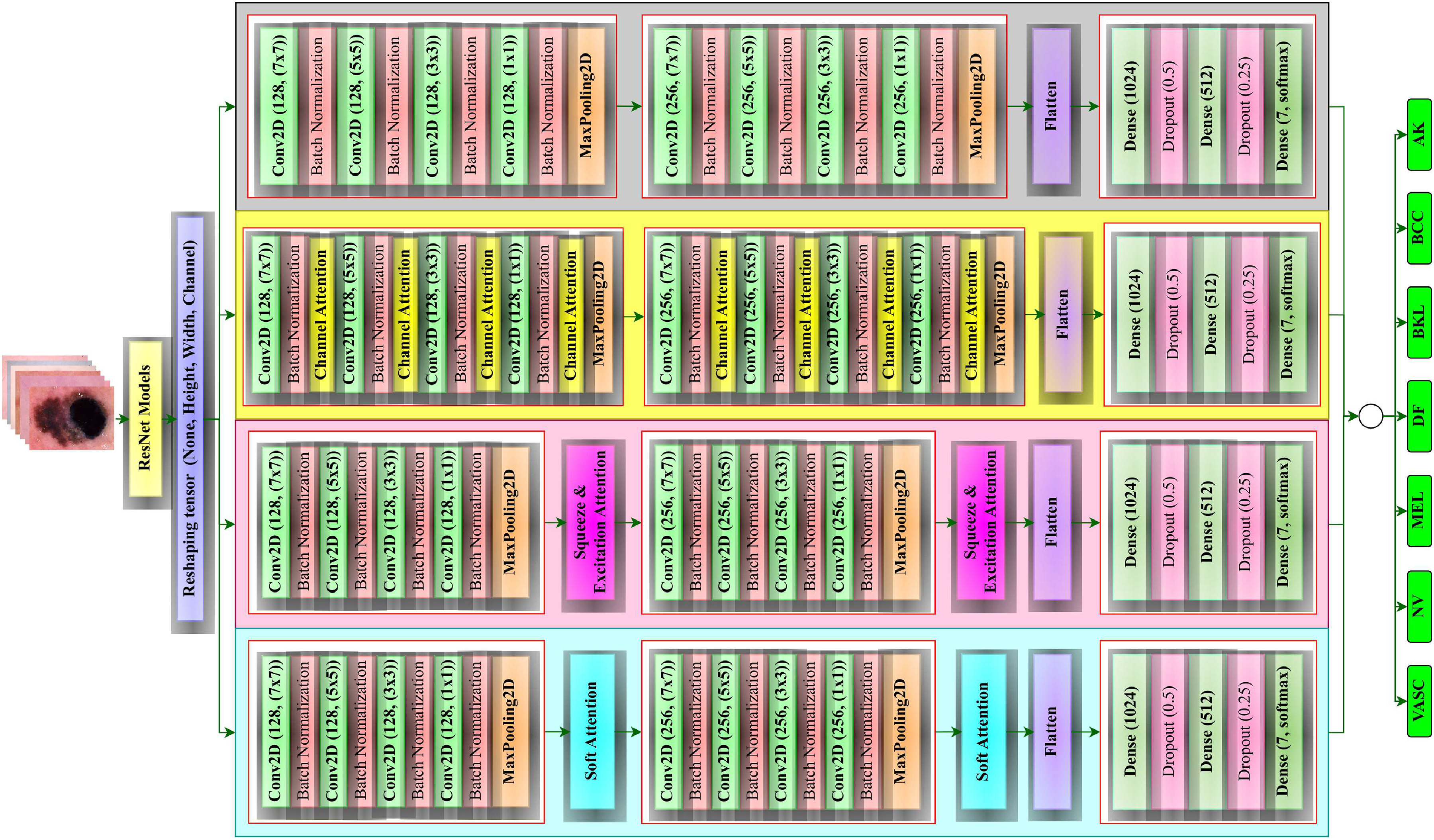
Customized ResNet variants (CRV) architecture for each variant of ResNet.
CRVs with fundamental fine tuning blocks
The process of integrating pre-trained models with our C_CNN, CA_CNN, SEA_CNN, or SA_CNN began by importing the pre-trained model from the ’keras’ library. Subsequently, the model was instantiated with our unique input shape and its output was transformed into a four-dimensional structure: none, height, width, and the number of channels. This adjustment was necessary to align our model with the pre-trained one, as our model required a four-dimensional input while the pre-trained model’s output tensor contained only two dimensions.
Following this, the fine-tuning process was initiated and carried out in a step-by-step manner. The culmination of this process involved recording predictions from each individualized model for subsequent analysis.
Conception of fundamental fine tuning blocks by customized CNN with attention triad
Our C_CNN architecture was structured with two sets of convolution blocks, each containing varying number of filters. Within each block, four “Conv2D” layers were incorporated with different kernel sizes: (7
To incorporate the CA module into CA_CNN, the process involved integrating this CA Layer within each convolution block, as described in the preceding paragraph. This integration entailed adding the CA layer after each “Conv2D” layer, alongside its corresponding “Batch Normalization” layer. The placement of the CA Layer between successive “Conv2D” layers served to refine features at an intermediate stage of convolutional processing. This arrangement facilitated the selective emphasis on significant channel-wise information and the suppression of less relevant details before proceeding with further processing.
When incorporating the SEA module to construct SEA_CNN, the process entailed embedding the SEA layer after each convolution block, following the organizational approach outlined in C_CNN. The SEA layer, incorporated after each convolution block, was tasked with recalibrating the feature responses across all channels. Its placement at this juncture facilitated the high-level adjustment of channel-wise importance following multiple convolutional operations, thereby augmenting the model’s ability to capture intricate and hierarchical features.
In integrating the SA module to configure SA_CNN, the inclusion of the SA layer followed a methodology akin to that of SEA_CNN, positioned after each convolution block. By situating SA layers after each block, the model was enabled to capture intricate patterns within the feature maps. However, owing to the heightened number of parameters within the internal organization upon the addition of SA, this layer was not deployed after every “Conv2D” layer.
The output obtained from the final max-pooling layer of each architecture was flattened and fed into a sequence comprising three fully connected layers. In this arrangement, a single fully connected block was introduced, incorporating three “Dense” layers with tensor dimensions of 1024, 512, and seven (corresponding to the number of classes). The first two fully connected layers utilized the “ReLU” activation function, while the final layer employed the “softmax” activation function to predict class probabilities. Furthermore, an additional layer of complexity was introduced to the initial two dense layers by incorporating “Dropout” mechanisms, aimed at preventing overfitting and regularization. This process commenced with a dropout rate of 50% in the first layer, followed by a 25% rate in the subsequent one.
Justification of attention triad integration for fine-tuning
Our methodology uses all ResNet variants as foundational feature extractors. These models are chosen due to their proven capability in handling complex image data, specifically in terms of hierarchical feature extraction across varying network depths. Using different ResNet architectures provides a comprehensive feature set by leveraging layers that progressively capture low-level textures, mid-level shapes, and high-level object representations. This multi-scale feature capture is essential for the nuanced task of skin lesion classification, where subtle texture and shape variations play a crucial role in diagnosis.
Data reshaping and model input preprocessing
To enhance the effectiveness of feature extraction, the input images are reshaped to a fixed dimension compatible with the ResNet input requirements. Reshaping not only standardizes image sizes, ensuring uniformity across the dataset, but also allows the models to optimally process spatial information. This standardization step is critical because skin lesion images may vary in resolution and scale, which can hinder model performance if not appropriately normalized.
When an image is passed through a pretrained ResNet model, the output tensor typically has the shape (none, C), where C denotes the number of channels or feature dimensions extracted by the model. This output shape, which is a flattened tensor, is suitable for passing directly into fully connected (dense) layers if the goal is straightforward classification. However, for our approach, which includes further fine-tuning and additional convolutions, this output needs to be reshaped to be compatible with 2D convolutional layers. Specifically, to enable the application of further convolutional operations on the output, the tensor must be reshaped into the format (none, height, width, and channels).
Here is a breakdown of the necessary steps to enable this:
Extracting feature maps with spatial dimensions: To apply fine-tuning via additional convolutional layers, we modify the ResNet models by not fully flattening the final convolutional layer’s output. Instead, we extract feature maps from an intermediate layer in the ResNet model, preserving the spatial dimensions (height and width) of the feature maps. This layer typically outputs a tensor shape, such as (none, 7, 7, and 2048) for ResNet50, where 2048 represents the number of channels. Reshaping the output for convolutional layers: Once we obtain the spatial feature maps, we reshape them as needed to maintain (none, height, width, and channels) format. This reshaping is essential because 2D convolutional layers expect a four-dimensional input with batch size, height, width, and channel dimensions. With this format, we can now apply additional convolutional layers to further process and refine features in a spatial context, which helps capture finer details relevant for skin lesion classification.
Channel attention
The CA mechanism selectively emphasizes the most informative channels within feature maps. In each ResNet layer, CA processes feature maps to assign higher weights to channels that contribute significantly to classification accuracy while suppressing less informative ones.
In our model, CA modules are added after the convolutional layers in the ResNet blocks. The channel importance is derived using global average pooling to aggregate spatial information, followed by a fully connected layer that outputs weights for each channel. By recalibrating channels, CA enables the model to focus more on discriminative skin lesion features, leading to more robust feature maps.
Squeeze-excitation attention
The squeeze-excitation mechanism enhances the representational power of a network by dynamically recalibrating channel-wise feature responses. SEA captures global information by first “squeezing” spatial dimensions through global average pooling, then “exciting” channels by learning non-linear relationships through a fully connected layer.
In our ResNet architecture, SEA modules are inserted after each residual block. The recalibration provides a refined weighting that allows the network to prioritize lesion features over background noise. This global channel-wise adaptation improves the sensitivity of the model to fine-grained lesion details, enhancing the model’s ability to differentiate between subtle variations in skin lesion patterns.
Soft attention
Unlike CA and SEA, which operate on channels, SA works on spatial features. It allows the model to selectively focus on specific regions within an image, particularly those with high diagnostic importance, such as lesion boundaries.
SA is applied following each ResNet block by generating attention maps that highlight important spatial areas. This spatial attention mechanism assigns higher weights to pixels or regions critical for skin lesion classification, enabling the model to concentrate on areas of interest while ignoring irrelevant parts of the image. This focus on essential spatial regions further improves feature discrimination.
Finally, after feature extraction and classification by each attention-integrated ResNet variant, we combine their predictions using IGIA. IGIA weights each model’s predictions inversely to its Gini index, prioritizing models with more even distribution in prediction confidence across classes. This ensemble technique reduces overfitting and enhances the generalization ability of our model, yielding a balanced and accurate classification output. The details of IGIA integration is described in the “IGIA” section.
Feature extraction process
We employed a TL model ResNet, which was pretrained on ImageNet for feature extraction, excluding the top fully connected layers (include_top = False) and using global average pooling (pooling = ‘‘avg’’). The output was reshaped to (16, 16, 8) before being processed through a series of convolutional layers with filter sizes of 7
Figure 6 illustrates the feature map activations at different layers of a TL model, specifically an example of a customized ResNet152 architecture. Each row corresponded to activations from a distinct layer in the model.
Input layer (input_1): The initial input image after preprocessing, showing the raw pixel data. Zero padding (zero_padding2d): Feature maps after applying zero padding to the input tensor, preparing it for convolution operations. Convolution (conv2d): Activation maps after passing through a convolutional layer with 64 filters, highlighting learned patterns and edges. Batch normalization (batch_normalization): Normalized feature maps following batch normalization, enhancing training stability, and convergence. ReLU activation (activation): Output after applying rectified linear unit (ReLU) activation function, introducing non-linearity to the network. Max-pooling (max_pooling2d): Downsampled feature maps post max-pooling, reducing spatial dimensions while retaining important features. Concatenation (concatenate): Activation maps after concatenating feature maps from previous layers, integrating information from multiple paths. Dense layer (dense): Feature maps transformed into a vector representation before entering the fully connected dense layer. Output layer (dense_1): Final layer activations depicting class probabilities through a softmax activation function.
Each subplot displayed up to seven filters per layer, visualized using the “viridis” colormap for clarity. The figure provided insights into how the model processed and transformed input images through successive layers, capturing hierarchical features crucial for classification tasks.
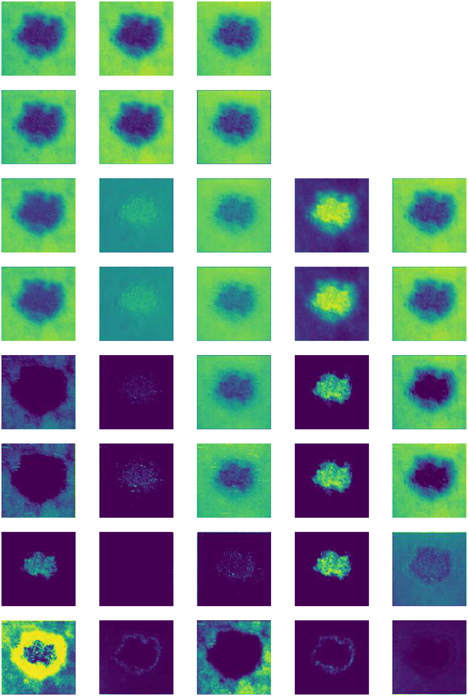
Feature extraction after activation of each layer (one image as example).
This exemplified a single sample and a subset of layers. Through this approach, we extracted thousands of feature images that significantly enhanced algorithm performance.
Attention triad (AT)
Our study employed three attention mechanisms to emphasize the most crucial input features as well as discard irrelevant ones.
Channel attention
The CA mechanism enhances feature maps by computing attention weights specific to each channel using mean and standard deviation calculations. These weights are then utilized to highlight crucial features within input feature maps.
33


Squeeze and excitation attention
The SEA module integrates both spatial dimension reduction and channel-wise attention learning operations. 34
Let 


Soft attention
SA allocates weights to input elements, concentrating on specific regions based on their relative significance.
30

Inverse Gini indexed averaging
We introduced a novel ensemble learning technique named inverse Gini indexed averaging (IGIA). This method computed optimal weights for predictions from individual classifiers and aggregated them through averaging, taking into account these weights. To accomplish this, we utilized the concept of the Gini index (GI), which was inverted afterward.
The theoretical justification of the IGIA method lies in its innovative adaptation of the GI to quantify prediction impurity and the introduction of the inverse GI (IGI) as a certainty-based metric. By inverting impurity through
The step-by-step process for implementing IGIA was delineated as follows:
This method initiated by evaluating the GI of predictions generated by individual classifiers. To achieve this, correctly classified samples were labeled as the class “1,” while incorrectly classified ones were marked as “0.” The GI was a measure of impurity or purity in a distribution. A lower GI indicated better separation and purity of the results. The approach calculated the GI for a set of predicted labels and then derived the IGI using a level of ensemble exponent ( The GI was calculated using the function In our method, the parameter This approach provided a measure of the predictive performance, with a lower GI indicating better prediction quality, and the IGI offering an alternative perspective on the predictive power of the model. Upon obtaining the IGI values for each classifier, we proceeded to compute the ensemble weights. These weights were derived by evaluating the ratio of each classifier’s information gain to the overall information gain. This method of weighting guaranteed that classifiers exhibiting greater information gains exerted a more pronounced influence on the ensemble. Ultimately, the predictions were averaged using the respective weights, resulting in a fused outcome that leveraged the strengths of each classifier within the ensemble. This process can be outlined as follows: let In summary, the IGIA ensemble method merges the predictions of individual architectures through weighted averaging, with weights assigned according to their respective performance or significance, as determined by the notion of information gain. The overall procedure of the IGIA technique is depicted in Figure 7.


Level wise inverse Gini indexed averaging (IGIA) (n = current level).
Multi-leveled IGIA
We structured our implementation of the IGIA technique across multiple tiers, a choice made to address the challenge of allocating sufficient emphasis to a particular superior model within a single tier due to the low individual classifier weights. As a solution, we adopted a sequential level-by-level ensembling strategy. This approach allowed us to highlight different models that exhibited superior performance compared to others at each tier. Consequently, this emphasis was further amplified through subsequent ensembling of these optimized models in later tiers. We provided a detailed explanation of our level-by-level approach in the following sections, while the overall visual representation of ML-IGIA is illustrated in Figure 8.
In this stage, the predictions obtained from the four base models (C_CNN, CA_CNN, SEA_CNN, and SA_CNN) were combined through ensembling for each classifier. This resulted in a total of 13 predictions derived from the initial tier across each of the CRV architectures, including RN50, RN101, RN152, RN50v2, RN101v2, RN152v2, RNRS50, RNRS101, RNRS152, RNRS200, RNRS270, RNRS350, and RNRS420. The 13 predictions produced in Level 1 were combined, resulting in six predictions at Level 2. These predictions stemmed from different versions of ResNet: RN from RN50, RN101, and RN152; RNv2 from RN50v2, RN101v2, and RN152v2; and RNRS from RNRS50, RNRS101, RNRS152, RNRS200, RNRS270, RNRS350, and RNRS420. Furthermore, composite predictions were formed by integrating all versions of RN50 (RN50, RN50v2, and RNRS50), resulting in RN50av (ResNet50_all_versions). Likewise, predictions were consolidated from all versions of RN101 (RN101, RN101v2, and RNRS101) to produce RN101av (ResNet101_all_versions), and from all versions of RN152 (RN152, RN152v2, and RNRS152) to yield RN152av (ResNet152_all_versions). From Level 2, the six predictions were further amalgamated to produce two additional runner-up predictions, which played a crucial role in determining the outcome in the subsequent level. Precisely, an ensemble was formed by merging RN, RNv2, and RNRS to create e_RN (ensembled_RN), while RN50av, RN101av, and RN152av were combined to form RN_av. The final prediction at the ultimate level, denoted as u_RN, was derived by combining the ensembled predictions e_RN and RN_av, which consistently yielded superior results compared to any other predictions.

Organization of multi-leveled inverse Gini indexed averaging (ML-IGIA).
Performance evaluation measures
To assess the performance and effectiveness of our models, a range of metrics such as accuracy, precision, recall (sensitivity), F1-score, specificity, and the ROC-AUC (receiver operating characteristic area under curve) were utilized, providing valuable insights into their predictive capabilities. These metrics were derived from the confusion matrix, a summary table outlining the model’s predictions relative to true positives, false positives, true negatives, and false negatives. The mathematical formulas for these metrics are detailed below:


Experimental setup
Our complete architecture was implemented on a Kaggle notebook, utilizing a GPU P100 for accelerated processing along with a 2-core Intel Xeon CPU, achieving an efficient runtime of 690 ms/step. For data preparation, we resized each lesion image to (224, 224, 3), ensuring compatibility with ResNet input requirements. The dataset was partitioned rigorously: 70% of images were used for training, 15% for validation, and the remaining 15% for testing. This fixed split enables us to evaluate the model’s generalizability effectively, and we did not apply cross-validation due to resource constraints and the stability of our dataset in this configuration.
To optimize model performance, we trained each ResNet variant for 50 epochs with a batch size of 16. We utilized the Adam optimizer, which provides adaptive learning rates for efficient convergence, initialized with a learning rate of 0.001. This rate was chosen after manual hyperparameter tuning to balance convergence speed and stability. We applied categorical cross-entropy for loss computation, appropriate for our multiclass classification task. To further improve robustness and prevent overfitting, we used early stopping with a Reduce on Plateau mechanism, which reduces the learning rate after 25 epochs without improvement. This strategy stabilizes training and preserves computational efficiency.
Trainable parameters
The IGIA ensemble functions exclusively during the prediction phase, ensuring that the total number of trainable parameters remains unchanged across different configurations, regardless of ensemble integration. Table 2 presents these parameters for each model variant and attention mechanism. Additionally, all algorithms required 3424 steps per epoch, with their respective training times also detailed in the table.
Trainable parameters and average training time (ATT) per step for each epoch for different algorithms.

C_CNN: customized convolutional neural network; CA_CNN: channel attention-based convolutional neural network; SEA_CNN: squeeze and excitation attention-based convolutional neural network; SA_CNN: soft attention-based convolutional neural network.
Among these, RNRS420 has the highest parameter count,
Hyperparameter selection
Hyperparameters, including learning rate, batch size, and early stopping criteria, were carefully selected through manual tuning based on established DL practices. Our chosen learning rate of 0.001 with the Adam optimizer provided reliable weight updates across our models, while batch normalization stabilized the training process and reduced overfitting risks. A “he_normal” initializer was employed for effective weight initialization, facilitating smooth gradient flow and accelerating model convergence. Additionally, the ReLU activation function enabled efficient capture of intricate data patterns, crucial for high classification accuracy in medical image analysis. This manual tuning approach, grounded in empirical observations, ensured a balance between computational efficiency and model performance, enhancing robustness and generalizability for the complex task of skin lesion classification.
Experimental results analysis
This section provides an in-depth exploration of both theoretical concepts and visual presentations to analyze the classification performances. The primary objective of these findings is to confirm the efficacy of employing IGIA to improve performance. By presenting experimental results, including a wide range of evaluation metrics and visual representations such as ROC-AUCs and confusion matrices, a thorough comparison of different approaches discussed in earlier sections is enabled.
The application of IGIA with all classifiers at each level (
CRV architectures in Level 1
A total of 13 models mentioned earlier were employed, which were paired with C_CNN, CA_CNN, SEA_CNN, and SA_CNN for each model variant. The outcomes obtained from these diverse combinations, along with the results from Level-1 IGIA, are presented in Tables 3 to 5.
Performances of ResNet architectures (Level 1).

Acc: accuracy; Pre: precision; Re: recall; F1: F1-score; Spe: specificity; C_CNN: customized convolutional neural network; CA_CNN: channel attention-based convolutional neural network; SEA_CNN: squeeze and excitation attention-based convolutional neural network; SA_CNN: soft attention-based convolutional neural network; IGIA: inverse Gini indexed averaging.
Performances of ResNetv2 architectures (Level 1).

Acc: accuracy; Pre: precision; Re: recall; F1: F1-score; Spe: specificity; C_CNN: customized convolutional neural network; CA_CNN: channel attention-based convolutional neural network; SEA_CNN: squeeze and excitation attention-based convolutional neural network; SA_CNN: soft attention-based convolutional neural network; IGIA: inverse Gini indexed averaging.
Performances of ResNetRS architectures (Level 1).

Acc: accuracy; Pre: precision; Re: recall; F1: F1-score; Spe: specificity; C_CNN: customized convolutional neural network; CA_CNN: channel attention-based convolutional neural network; SEA_CNN: squeeze and excitation attention-based convolutional neural network; SA_CNN: soft attention-based convolutional neural network; IGIA: inverse Gini indexed averaging.
Table 3 presents the classification performance of various attention mechanisms integrated into all ResNet version-1 architectures (RN50, RN101, and RN152).
Analyzing the results for RN50, it is observed that ResNet50 with C_CNN blocks delivered better performance than the attention mechanism integrated C_CNN blocks. ResNet50 with C_CNN blocks achieved the highest 91.91% accuracy, whereas the SA_CNN integrated ResNet50 delivered the lowest 89.61% accuracy. In terms of precision, ResNet50 with C_CNN blocks achieved the highest precision of 91.51%, indicating that out of all the items identified or predicted as positive by this model, 91.51% were true positives. Regarding recall values, ResNet50 with C_CNN blocks achieved the highest recall of 91.91%, indicating that out of all the actual positive items in the dataset, 91.91% were correctly identified by the model. In terms of the F1-score, C_CNN-integrated ResNet50 performed better with a score of 91.47%, reflecting a high level of performance in both precision and recall. For specificity, ResNet50 integrated with C_CNN provided the highest value of 84.23%, referring to the proportion of true negatives correctly identified by the model. However, after integrating Level-1 IGIA into all these architectures, we observed a significant improvement in all measures except specificity: 92.27% accuracy and recall, 91.81% precision, 91.78% F1-score, and 83.77% specificity.
For RN101, a different scenario was observed where CA_CNN and SA_CNN integrated architectures outperformed C_CNN, while SEA_CNN did not. Specifically, C_CNN obtained 91.18% accuracy, whereas CA_CNN and SA_CNN achieved 91.67%, with SEA_CNN having the least at 89.61%. In terms of precision, recall, F1-score, and specificity, CA_CNN and SA_CNN consistently outperformed C_CNN, with SEA_CNN lagging. However, after integrating Level-1 IGIA into all these architectures, we observed the same trend as with RN50, showing significant improvements in all metrics except specificity. The Level-1 IGIA integration resulted in 93.24% accuracy and recall, 93.17% precision, 92.87% F1-score, and 84.74% specificity.
For RN152, the integration of attention mechanisms led to performance improvements over C_CNN blocks. Specifically, RN152 with CA_CNN and SA_CNN blocks showed better performance compared to C_CNN. After integrating Level-1 IGIA into RN152, we found enhanced performance across all metrics. RN152 achieved 93.00% accuracy, 92.58% precision, 93.00% recall, 92.66% F1-score, and 85.71% specificity. This demonstrates that RN152 with attention mechanisms and Level-1 IGIA integration outperformed the C_CNN blocks in all performance measures.
Analyzing the results for RN50v2, it was observed that ResNet50v2 with SEA_CNN blocks delivered the best performance among the various attention mechanism integrated C_CNN blocks. Specifically, SEA_CNN achieved the highest accuracy of 90.46%, whereas SA_CNN had the lowest accuracy at 89.13%. In terms of precision, SEA_CNN also led with 89.70%, meaning that 89.70% of the items identified as positive by this model were true positives. SEA_CNN maintained its lead in recall as well, with 90.46%, indicating that 90.46% of the actual positive items in the dataset were correctly identified. SEA_CNN’s F1-score was the highest at 89.92%, showing a strong balance between precision and recall. However, SA_CNN demonstrated the highest specificity at 83.55%, referring to the proportion of true negatives correctly identified. After integrating Level-1 IGIA into RN50v2, there were substantial improvements across all metrics except specificity. Specifically, RN50v2 with Level-1 IGIA achieved 92.15% accuracy, 91.47% precision, 92.15% recall, 91.51% F1-score, and 82.81% specificity.
For RN101v2, CA_CNN and SA_CNN integrated architectures outperformed C_CNN and SEA_CNN blocks. CA_CNN achieved the highest accuracy of 91.30%, while C_CNN had 90.10%, and SEA_CNN and SA_CNN achieved 90.82% and 90.46%, respectively. In terms of precision, CA_CNN again led with 90.99%, indicating a higher proportion of true positives among those identified as positive. CA_CNN also achieved the highest recall of 91.30%, suggesting better identification of actual positive items. The F1-score for CA_CNN was 91.06%, reflecting strong overall performance. Specificity was highest for CA_CNN as well at 87.06%, indicating accurate identification of true negatives. After integrating Level-1 IGIA, RN101v2 showed notable improvements, achieving 92.75% accuracy, 92.42% precision, 92.75% recall, 92.41% F1-score, and 85.70% specificity.
For RN152v2, the use of CA_CNN and SA_CNN blocks led to better performance compared to C_CNN. CA_CNN and SA_CNN both achieved higher accuracy (90.94%) compared to C_CNN (89.73%) and SEA_CNN (90.58%). CA_CNN also led in precision (90.28%) and recall (90.94%), indicating better identification of true positives and actual positive items. The F1-score for CA_CNN was the highest at 90.40%, reflecting a balance between precision and recall. Specificity was highest for C_CNN at 85.99%, showing a good rate of true negative identification. After integrating Level-1 IGIA, RN152v2 showed improved performance across all metrics: 92.15% accuracy, 91.63% precision, 92.15% recall, 91.65% F1-score, and 85.68% specificity.
Similarly, when describing the RenNetRS architectures and their Level-1 IGIA performance, we observed a mixed scenario with the use of AT. However, utilizing IGIA provided a perfect scenario.
RNRS50 with SA_CNN blocks achieved the highest accuracy at 91.30%, and also excelled in precision (90.89%) and recall (91.30%). However, integrating Level-1 IGIA into RNRS50 resulted in the best performance overall, with an accuracy of 93.48%, precision of 93.12%, recall of 93.48%, F1-score of 93.00%, and specificity of 85.30%.
For RNRS101, SA_CNN delivered the highest accuracy at 91.43%, while SEA_CNN followed closely with 91.06%. Precision, recall, and F1-score were highest for SEA_CNN (90.96%, 91.06%, and 90.93%, respectively). With Level-1 IGIA, RNRS101 improved further to 92.27% accuracy, 91.90% precision, 92.27% recall, 91.99% F1-score, and 85.22% specificity.
RNRS152 with SEA_CNN blocks performed the best in accuracy (92.51%), precision (92.04%), recall (92.51%), and F1-score (92.04%). Level-1 IGIA integration enhanced these metrics further, achieving 93.12% accuracy, 92.69% precision, 93.12% recall, 92.57% F1-score, and 84.77% specificity.
For RNRS200, the highest accuracy was observed with Level-1 IGIA integration, achieving 93.60%, along with 93.19% precision, 93.60% recall, 93.16% F1-score, and 84.80% specificity. SEA_CNN also performed well, with 91.91% accuracy and 91.60% precision.
RNRS270 with Level-1 IGIA outperformed other blocks, reaching 93.24% accuracy, 92.93% precision, 93.24% recall, 92.77% F1-score, and 83.81% specificity. CA_CNN showed strong specificity at 86.10%.
The highest accuracy for RNRS350 was with Level-1 IGIA, achieving 92.63%. SEA_CNN delivered high performance in recall (90.58%) and precision (90.32%). SA_CNN had notable specificity at 87.11%.
Level-1 IGIA integration provided the best results for RNRS420 with 92.15% accuracy, 91.61% precision, 92.15% recall, 91.43% F1-score, and 83.75% specificity. CA_CNN showed the highest specificity at 88.97%.
CRV architectures in Level 2
At Level 2, our methodology entailed utilizing distinct combinations derived from the Level-1 predictions. To elaborate, the initial fusion involved the three ResNet models from the previous level IGIA: RN50, RN101, and RN152, appropriately denoted as “RN.” Moving forward, the “RNv2” configuration synchronized the predictive capabilities of RN50v2, RN101v2, and RN152v2. Finally, the composite ’RNRS’ amalgamation consolidated the predictive abilities of all versions of RNRS architectures, including RNRS50, RNRS101, RNRS152, RNRS200, RNRS270, RNRS350, and RNRS420 models. The results of these combinations are outlined in Table 6.
Performance metrics of Level-2 IGIA.

Acc: accuracy; Pre: precision; Re: recall; F1: F1-score; Spe: specificity; C_CNN: customized convolutional neural network; CA_CNN: channel attention-based convolutional neural network; SEA_CNN: squeeze and excitation attention-based convolutional neural network; SA_CNN: soft attention-based convolutional neural network; IGIA: inverse Gini indexed averaging.
Each of these models from the initial fusion individually showcased notable performance, as depicted by their respective accuracy, precision, recall, F1-score, and specificity metrics. However, when amalgamated into the composite “RN” configuration, their predictive capabilities were synchronized, resulting in enhanced performance. The composite “RN” configuration achieved an accuracy of 93.24%, precision of 92.90%, recall of 93.24%, F1-score of 92.76%, and specificity of 83.80%.
The “RNv2” configuration synchronized the predictive capabilities of the updated ResNet models (RN50v2, RN101v2, and RN152v2). Each of these models demonstrated improved performance over their predecessors, as evidenced by their Level-1 metrics. Upon synchronization into the “RNv2” configuration, their predictive power was further amplified. The composite “RNv2” configuration achieved an accuracy of 92.75%, precision of 92.23%, recall of 92.75%, F1-score of 92.28%, and specificity of 83.79%.
The “RNRS” amalgamation consolidated the predictive abilities of all versions of RNRS architectures (RNRS50, RNRS101, RNRS152, RNRS200, RNRS270, RNRS350, and RNRS420). These architectures were specifically designed to adapt and excel in varied scenarios. Individually, they exhibited commendable performance across different metrics. When integrated into the composite “RNRS” configuration, their combined predictive power was unleashed, resulting in impressive performance. The composite “RNRS” configuration achieved an accuracy of 93.48%, precision of 93.20%, recall of 93.48%, F1-score of 93.03%, and specificity of 84.78%.
This detailed description highlighted the synergistic effect of combining different ResNet architectures at Level 2 of the IGIA methodology, showcasing how each configuration leveraged the strengths of its constituent models to achieve superior predictive performance.
In contrast, our approach also involved incorporating the three iterations of RN50 architectures, namely RN50, RN50v2, and RNRS50. This amalgamated model was aptly labeled as “RN50av.” Similarly, the “RN101av” setup harmonized the predictive capacities of RN101, RN101v2, and RNRS101. Furthermore, the comprehensive “RN152av” integration consolidated the predictive capabilities of all iterations of RN152 architectures, encompassing RN152, RN152v2, and RNRS152. The outcomes of these amalgamations are detailed in Table 7.
Performance metrics of Level-2 IGIA.

IGIA: inverse Gini indexed averaging; Acc: accuracy; Pre: precision; Re: recall; F1: F1-score; Spe: specificity; C_CNN: customized convolutional neural network; CA_CNN: channel attention-based convolutional neural network; SEA_CNN: squeeze and excitation attention-based convolutional neural network; SA_CNN: soft attention-based convolutional neural network.
To be more specific, the “RN50av” setup amalgamated the predictive capacities of RN50, RN50v2, and RNRS50 architectures. Individually, these architectures demonstrated commendable performance across various metrics. Upon integration, their predictive capabilities were harmonized, resulting in enhanced performance. The composite ’RN50av’ configuration achieved an accuracy of 92.87%, precision of 92.40%, recall of 92.87%, F1-score of 92.38%, and specificity of 83.81%.
Similarly, the “RN101av” setup harmonized the predictive capacities of RN101, RN101v2, and RNRS101 architectures. These architectures showcased notable performance individually. When amalgamated into the “RN101av” configuration, their predictive capabilities were synchronized, resulting in improved performance. The composite “RN101av” configuration achieved an accuracy of 93.60%, precision of 93.32%, recall of 93.60%, F1-score of 93.28%, and specificity of 85.26%.
The “RN152av” integration consolidated the predictive capabilities of all iterations of RN152 architectures, encompassing RN152, RN152v2, and RNRS152. Each of these architectures demonstrated strong performance across various metrics. Upon integration, their predictive power was unleashed, resulting in enhanced overall performance. The composite “RN152av” configuration achieved an accuracy of 93.36%, precision of 92.92%, recall of 93.36%, F1-score of 92.85%, and specificity of 84.78%.
This detailed description elucidated how amalgamating different iterations of RN architectures at Level 2 of the IGIA methodology enhanced their predictive capabilities, resulting in improved overall performance across various metrics.
Notably, throughout this level, it is apparent that almost all the performance metrics’ values were increased than those of the former level.
CRV architectures in Level 3
In this tier, we encountered two ensemble predictions: “e_RN” derived from the previous level’s RN, RNv2, and RNRS, and “RN_all_versions” (RN_av) stemming from the preceding level’s RN50av, RN101av, and RN152av. The performance metrics for “e_RN” are illustrated in Table 8, while the results for “RN_av” are presented in Table 9.
Performance metrics of Level-3 IGIA (e_RN).
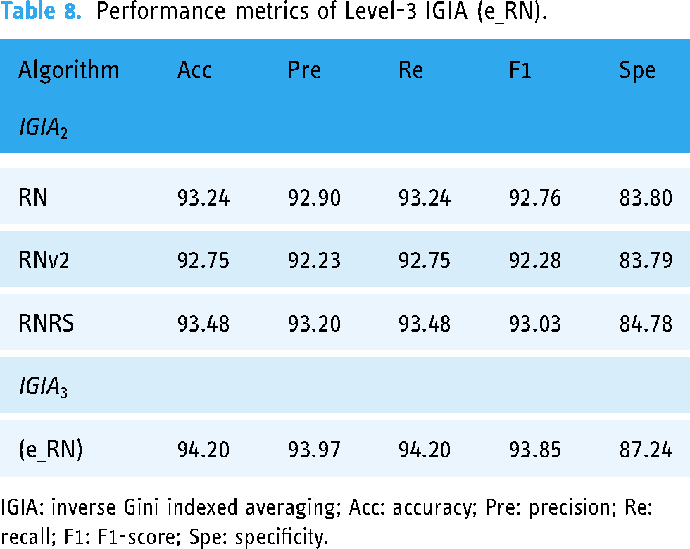
IGIA: inverse Gini indexed averaging; Acc: accuracy; Pre: precision; Re: recall; F1: F1-score; Spe: specificity.
Performance metrics of Level-3 IGIA (RN_av).
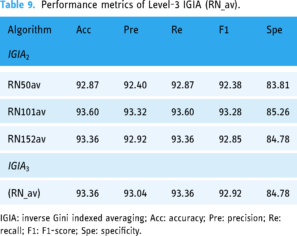
IGIA: inverse Gini indexed averaging; Acc: accuracy; Pre: precision; Re: recall; F1: F1-score; Spe: specificity.
The “e_RN” ensemble prediction was derived from the amalgamation of predictions from the previous level’s RN, RNv2, and RNRS architectures. Each of these architectures had demonstrated strong performance individually, as evidenced by their accuracy, precision, recall, F1-score, and specificity metrics. When combined into the “e_RN” ensemble, their predictive capabilities were synchronized, resulting in enhanced performance. The “e_RN” ensemble achieved an accuracy of 94.20%, precision of 93.97%, recall of 94.20%, F1-score of 93.85%, and specificity of 87.24%.
The “RN_av” ensemble prediction stemmed from the amalgamation of predictions from the preceding level’s RN50av, RN101av, and RN152av architectures. These architectures, representing different versions of RN architectures, exhibited commendable performance across various metrics. Upon integration into the “RN_av” ensemble, their predictive capabilities were harmonized, resulting in improved overall performance. The “RN_av” ensemble achieved an accuracy of 93.36%, precision of 93.04%, recall of 93.36%, F1-score of 92.92%, and specificity of 84.78%.
In summary, the ensemble predictions by IGIA at Level 3 of our methodology leveraged the strengths of individual architectures and synchronize their predictive capabilities to achieve superior performance.
CRV architectures in Level 4
In the final phase, we leveraged the predictive power of two selections obtained from Level 3. The meticulous examination of these three refined selections was undertaken, and the results obtained from this ultimate stage are presented in Table 10. Significantly, it became glaringly evident in this context that this ultimate level prediction surpassed all previous predictions across nearly all performance evaluation metrics.
Performance metrics of Level-4 IGIA (u_RN).

IGIA: inverse Gini indexed averaging; Acc: accuracy; Pre: precision; Re: recall; F1: F1-score; Spe: specificity.
Notably, this ultimate level prediction surpassed all previous predictions across nearly all performance evaluation metrics, underscoring the effectiveness of our iterative refinement process. The “u_RN” ensemble achieved an accuracy of 94.52%, precision of 94.16%, recall of 94.52%, F1-score of 93.96%, and specificity of 85.32%.
In summary, the CRV architectures at Level 4 represented the culmination of our iterative refinement process, where the predictive capabilities of the ensemble predictions from Level 3 were further optimized to achieve superior performance.
Statistical analysis by confidence intervals (CIs)
Table 11 presents the performance metrics of the proposed architecture, including accuracy, precision, recall, F1-score, and specificity, along with their 95% and 99% CIs. The model achieves an accuracy of 94.52%, with a CI range of 92.97%–96.07% (95%) and 92.48%–96.56% (99%), reflecting consistent performance. Precision and recall are similarly robust at 94.16% and 94.52%, respectively, with narrow CI ranges, highlighting the model’s reliability in predicting positive cases. The F1-score, a harmonic mean of precision and recall, stands at 93.96%, with CIs of 92.34%–95.58% (95%) and 91.83%–96.09% (99%). Specificity, although lower at 85.32%, also demonstrates reliability with a CI range of 82.91%–87.73% (95%) and 82.15%–88.49% (99%). These results emphasize the robustness of the proposed architecture under varying statistical confidence levels, ensuring its reliability in practical applications.
Performance metrics of the proposed architecture with 95% and 99% confidence intervals (CIs).

This representation ensures that the statistical reliability of the reported results is clearly communicated, strengthening the evaluation of the proposed approach.
Performance analysis by visualization
Confusion matrix
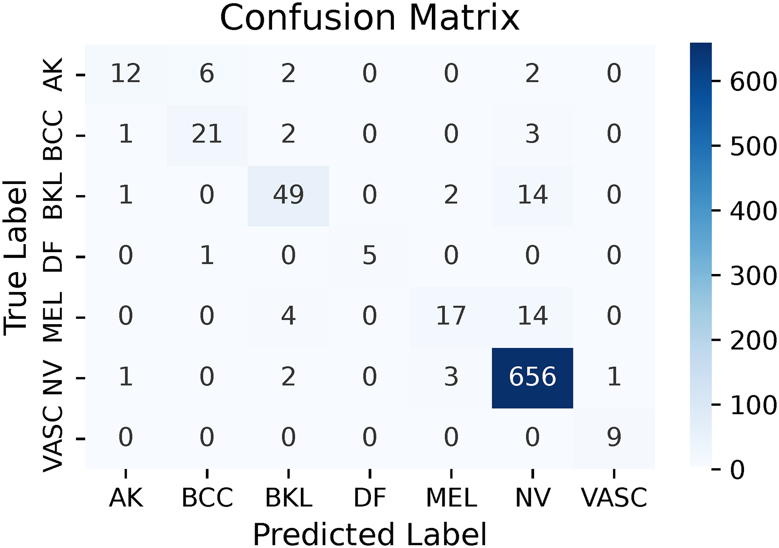
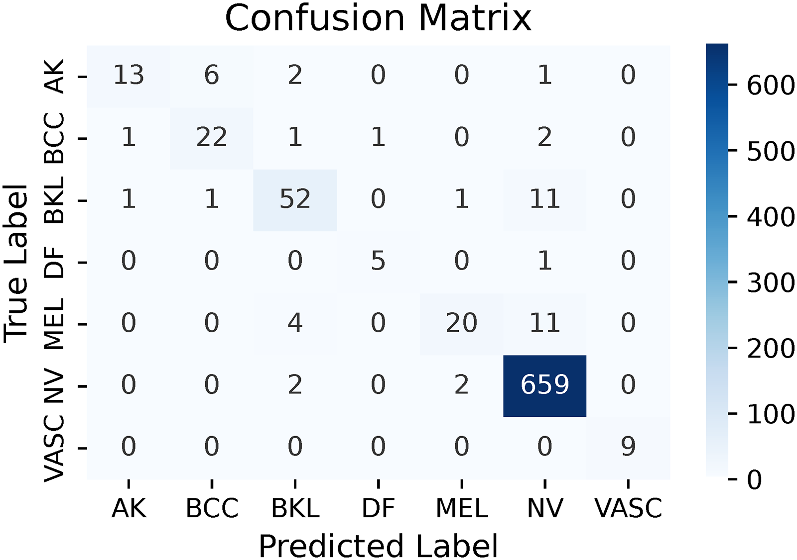
Due to the incorporation of a diverse number of classifiers, each with its unique variations, it was decided not to provide the confusion matrices for all individual classifiers from all levels of IGIA. Instead, emphasis was placed on displaying the confusion matrices resulting from the ML-IGIA approach from the second level to the final level. These visual representations, depicted from Figure 9 to 17, provided a concise illustration of the accuracy and error rates for each category. Furthermore, they confirmed the high performance of ML-IGIA in classifying samples across all categories.

Confusion matrix of RN (multi-leveled inverse Gini indexed averaging (ML-IGIA) Level 2).

Confusion matrix of RNv2 (multi-leveled inverse Gini indexed averaging (ML-IGIA) Level 2).

Confusion matrix of RNRS (multi-leveled inverse Gini indexed averaging (ML-IGIA) Level 2).
Confusion matrix of RN50av (multi-leveled inverse Gini indexed averaging (ML-IGIA) Level 2).

Confusion matrix of RN101av (multi-leveled inverse Gini indexed averaging (ML-IGIA) Level 2).

Confusion matrix of RN152av (multi-leveled inverse Gini indexed averaging (ML-IGIA) Level 2).
Confusion matrix of e_RN (multi-leveled inverse Gini indexed averaging (ML-IGIA) Level 3).

Confusion matrix of RN_av (multi-leveled inverse Gini indexed averaging (ML-IGIA) Level 3).

Confusion matrix of u_RN (multi-leveled inverse Gini indexed averaging (ML-IGIA) Level 4).
In Level 2, the RN architecture demonstrated good performance, as shown in Figure 9. For AK, the model correctly classified 12 samples and misclassified 10. BCC had 21 accurate identifications with six misclassifications. BKL achieved 50 correct classifications against 16 misclassifications. DF was correctly identified in five instances with just one misclassification. MEL had 18 correct predictions and 17 misclassifications, indicating some overlap with other categories. NV showed strong performance with 657 true positives and six misclassifications. VASC had perfect classification with all nine samples correctly identified. This performance highlighted the model’s effectiveness, with generally high true positive rates and areas for potential improvement.
Again, in Level 2, the RNv2 architecture showcased the following performance metrics as revealed in Figure 10. For AK, the model correctly classified 11 samples and misclassified the same number of samples. BCC had 21 accurate identifications with six misclassifications. BKL achieved 47 correct classifications against 19 misclassifications. DF was correctly identified in five instances with just one misclassification. MEL had 19 correct predictions and 16 misclassifications, reflecting some challenges in distinguishing this category. NV exhibited strong performance with 656 true positives and seven misclassifications. VASC had perfect classification with all nine samples correctly identified. These results indicated robust performance with high true positive rates, though some categories exhibited notable misclassification rates.
Another architecture named RNRS performed the best at this level, as depicted in Figure 11. AK was accurately classified in 13 instances, with nine samples misclassified. For BCC, 22 samples were correctly identified, while five were not, indicating solid performance. In the case of BKL, there were 50 correct classifications and 16 misclassifications. DF saw five correct identifications with just one misclassification. MEL, on the other hand, presented a challenge with 18 correct predictions and 17 misclassifications. NV stood out with 657 true positives against six misclassifications, showcasing excellent performance. VASC was perfectly classified, with all nine samples correctly identified, demonstrating high precision in this category.
As illustrated in Figure 12, the RN50av architecture showed strong performance as well. For AK, 12 samples were correctly classified, while 10 were misclassified, indicating a need for improvement in this category. BCC had 21 accurate predictions and six misclassifications, showing solid recognition. The BKL class had 49 correct identifications and 17 errors, suggesting reliable performance with some room for improvement. DF was well-identified with five correct classifications and only one misclassification. MEL had 17 true positives but 18 misclassifications, highlighting challenges in distinguishing it from other classes. NV was strongly predicted with 656 correct identifications and seven errors, showcasing the model’s proficiency. VASC achieved perfect classification with all nine samples correctly identified, indicating high precision.
In Level 2, another architecture (RN101av) exhibited the performance shown in Figure 13. For AK, there were 14 correct classifications and eight misclassifications, indicating moderate accuracy. BCC had 22 samples accurately identified and five misclassifications, showcasing solid recognition capabilities. The BKL class had 50 correct predictions and 16 errors, suggesting robust performance with a minor margin for error. DF was identified accurately in five instances with just one misclassification. MEL had 20 true positives but 15 misclassifications, highlighting challenges in distinguishing it from other classes. NV demonstrated strong prediction with 655 correct identifications and eight errors, reflecting the model’s proficiency. VASC achieved perfect classification with all nine samples correctly identified, demonstrating high precision.
The last architecture of Level 2, RN152av, showcased a mixed performance across different classes. It accurately identified 12 instances of AK but misclassified 10 cases, suggesting room for improvement. Conversely, BCC exhibited strong recognition capabilities with 22 correct identifications and only five misclassifications. Similarly, BKL demonstrated robust performance, correctly predicting 51 samples and misclassifying 15. DF showed flawless performance with all six instances correctly classified. However, MEL presented a challenge with 16 correct predictions but 19 misclassifications, indicating difficulty in distinguishing MEL from other classes. NV stood out with 657 correct identifications and only six errors, showcasing the model’s proficiency. Finally, VASC achieved perfect classification, correctly identifying all nine samples, highlighting high precision in VASC recognition.
In Level 3, the ensembled e_RN architecture significantly enhanced performance compared to Level 2, as evidenced by a notable reduction in misclassification rates. The confusion matrix revealed that for AK, the model correctly classified 13 samples while misclassifying nine, indicating some room for improvement. For BCC, 22 samples were accurately identified with only five misclassifications, showcasing robust recognition capabilities. The model achieved 52 correct classifications against 14 misclassifications for BKL, demonstrating strong performance with a minor margin for error. DF was correctly identified in five instances with just one misclassification, suggesting reliable identification despite the lower number of true positives. MEL presented a challenge with 20 correct predictions and 15 misclassifications, highlighting the need for further refinement due to overlapping features with other categories. NV stood out with an impressive 659 true positives and only four misclassifications, underscoring the model’s exceptional capability in identifying this class. Notably, VASC had perfect classification with all nine samples correctly identified, indicating high precision possibly due to its distinct feature set. The dominance of true positives across the confusion matrix signified the model’s effectiveness, with relatively low misclassifications highlighting its strong overall performance and potential for further enhancement. The pictorial representation is demonstrated in Figure 15.
In Level 3, the RN_av architecture showed a solid performance, though with slightly more room for improvement compared to the e_RN architecture. For AK, the model correctly classified 12 samples while misclassifying 10, indicating the need for better differentiation of this category. BCC saw 22 accurate identifications with five misclassifications, demonstrating strong, albeit slightly less robust, and recognition capabilities. BKL had 51 correct classifications against 15 misclassifications, showing good performance with some margin for error. DF was reliably identified with five true positives and just one misclassification. MEL presented a challenge, with 18 correct predictions and 17 misclassifications, suggesting significant overlap with other categories and a need for further refinement. NV continued to be the best-predicted class with 656 true positives and only seven misclassifications, highlighting the model’s exceptional ability to identify NV accurately. Lastly, VASC had a perfect classification with all nine samples correctly identified, indicating high precision likely due to its distinct features. This overall performance reflected a strong model, with effective true positive rates and some areas for enhancement, as illustrated in Figure 16.
The ultimate confusion matrix revealed insightful details about the model’s performance across different classes. Specifically, it highlighted 13 instances of true positives, indicating accurate classifications, whereas it also shed light on nine cases where AK was misclassified as other classes, suggesting potential areas for enhancement in accurately categorizing this class. BCC exhibited 23 true positives with relatively few misclassifications, indicating decent accuracy in identification, albeit more flawless than AK. The BKL class boasted 53 true positives, showcasing the model’s strong capability in identifying this class with minimal misclassifications. Conversely, the DF class recorded only five true positives, possibly due to fewer DF samples in the dataset, though there existed only a single misclassification. MEL demonstrated 20 true positives, suggesting satisfactory predictive performance, albeit with 13 misclassifications, likely owing to feature similarities with other classes. NV emerged as the most successfully predicted class, with an impressive 658 true positives and merely five misclassifications, underscoring the model’s proficiency in identifying NV. Intriguingly, the VASC class registered no misclassifications, although the exact count of true positives remained only six. This anomaly could have stemmed from either a limited VASC sample size in the dataset or distinct features that the model could easily distinguish. Overall, the predominance of diagonal values in the confusion matrix signified a substantial number of true positives, indicative of the model’s efficacy in making accurate predictions. The sparse off-diagonal values denoted misclassifications, which were relatively minimal for most classes, implying a well-performing model. However, the varying sample sizes across classes may have influenced precision and recall metrics, necessitating careful consideration in evaluating the model’s effectiveness.
Receiver operating characteristic area under curve (ROC-AUC)
The ROC-AUC served as a powerful visualization tool for assessing the model’s performance. Hence, an evaluation of this metric was carried out. Graphical representations of the ROC-AUC for the ML-IGIA approach at the ultimate level (Level 4) is presented in Figure 18. This curve revealed a notable observation: minimal fluctuation was observed across each class, indicating a consistently strong performance by the model.

ROC-AUC curve obtained by ML-IGIA (Level 4). ROC-AUC: receiver operating characteristic area under curve; ML-IGIA: multi-leveled inverse Gini indexed averaging.
Gradient class activation map (GradCAM)
GradCAM was implemented as a visualization technique to enhance the interpretability of the proposed model by highlighting the regions of input images that contributed most to the predictions. The final convolutional layer of the model was selected as the target for generating activation maps, as this layer was expected to capture high-level spatial features.
Figure 19 demonstrates the stepwise flow of implementaion of GradCAM visualization where the methodology began with the construction of a gradient model that mapped input images to both the output of the last convolutional layer and the model’s final predictions. The gradient of the class-specific output score with respect to the activations of the selected convolutional layer was calculated using TensorFlow’s GradientTape. These gradients were pooled spatially by computing the mean intensity for each feature map channel, signifying the importance of each channel for the target class.

Step-by-step implementation of gradient class activation map (GradCAM) visualization.
The activation maps of the final convolutional layer were then weighted by the pooled gradients and aggregated to produce a class activation heatmap. The heatmap was normalized to a range between 0 and 1 for visualization purposes. The original input image and the heatmap were overlaid using a colormap to illustrate the regions that influenced the model’s decision.
This approach was extended to multiple classes by iterating through the test dataset, selecting images from each class, and visualizing their GradCAM outputs. The generated heatmaps revealed that the model effectively focused on salient regions associated with the target classes, such as lesions in medical images, indicating its ability to identify optimal regions of interest.
The interpretability provided by GradCAM facilitated an in-depth understanding of the model’s decision-making process. By visually confirming the regions of interest, the technique demonstrated that the model made predictions based on relevant features, thereby increasing its reliability and transparency for end-users.
The visualization for each class is depicted in Figure 20, where instances from seven different classes were selected, and their corresponding GradCAM view was juxtaposed with the original image. This illustration showcased the model’s proficiency in pinpointing precise regions within each image that held greater significance, thus enhancing its classification accuracy.

GradCAM generation by the model for each class. (a) AK, (b) GradCAM, (c) BCC, (d) GradCAM, (e) BKL, (f) GradCAM, (g) DF, (h) GradCAM, (i) MEL, (j) GradCAM, (k) NV, (l) GradCAM, (m) VASC and (n) GradCAM. GradCAM: gradient class activation map; AK: actinic keratosis; BCC: basal cell carcinoma; BKL: benign keratosis; DF: dermatofibroma; MEL: melanoma; NV: nevus; VASC: vascular lesions.
However, Grad-CAM has limitations. It relies heavily on model predictions, meaning any misclassification by the model can lead to incorrect or misleading heatmaps. Additionally, for complex or subtle skin lesions, Grad-CAM may sometimes highlight irrelevant regions, reducing its reliability in ambiguous cases.
To enhance comprehension, it was crucial to note that an accurate heatmap generated by a model, which effectively covered the relevant region, signified the model’s capability to make correct classifications. Conversely, an incorrect heatmap suggested potential inaccuracies in the model’s classifications. To illustrate this concept further, an example is depicted in Figure 21.

GradCAM visualization for architecture explainability (example by RN50 model): (a) original, (b) CA_CNN, (c) SEA_CNN, (d) SA_CNN. GradCAM: gradient class activation map; C_CNN: customized convolutional neural network; CA_CNN: channel attention-based convolutional neural network; SEA_CNN: squeeze and excitation attention-based convolutional neural network; SA_CNN: soft attention-based convolutional neural network.
In Figure 21, an exemplary image representing the NV class is presented. Notably, the attention-based architectures, as executed by RN50, effectively identified the relevant region of interest. Furthermore, the involvement of additional models served to reinforce this claim. By integrating multiple models, the final prediction consistently proved to be accurate. This fact became apparent upon examining the GradCAM visualizations of these supplementary models, providing further validation. However, a notable innovation came into play with the IGIA ensemble, enabling precise class predictions. This observation underscored the effectiveness of the advanced ML-IGIA technique, demonstrating its ability to surpass individual classifier limitations and affirm its superiority in delivering accurate predictions.
Ablation study
To demonstrate the superiority of our novel approach compared to state-of-the-art methods, we conducted a comprehensive ablation study focusing on two key innovations: AT and IGIA. We evaluated the performance impact of these components by analyzing the results with and without their utilization.
Utilization of IGIA without TA
We applied IGIA across all variants of ResNet models, including ResNet, ResNetv2, and ResNetRS, at different levels as previously mentioned. Each model was tested in four configurations: three with AT and one without attention modules. To highlight the efficacy of AT, we presented the results in Table 12, showcasing the performance of IGIA excluding the TA-integrated models and compared them with our proposed architecture.
Performance metrics of IGIA without AT.

IGIA: inverse Gini indexed averaging; AT: attention triad; Acc: accuracy; Pre: precision; Re: recall; F1: F1-score; Spe: specificity.
Our proposed IGIA demonstrated superior performance when enhanced with AT compared to traditional IGIA and other ensembling methods. By incorporating AT into IGIA, our approach, presented as “Ours” in the table, achieved the highest accuracy of 94.52%, surpassing the performance of all other configurations. This significant improvement underscored the efficacy of AT in refining IGIA’s ability to aggregate model predictions, leading to more accurate and reliable outcomes.
Without AT, various levels of IGIA implementations yielded commendable results. Among them,
Utilization of conventional ensemble methods instead of IGIA
As previously mentioned, we applied IGIA at multiple levels using a distinct approach. Predictions from C_CNN, CA_CNN, SEA_CNN, and SA_CNN models were ensembled by determining the optimal weights for all models as well as for the top three models. Specifically, IGIA utilizing all classifiers at level
Softmax averaging
As shown in Table 13, SA using all classifiers at level
Performance metrics of softmax averaging of all classifiers.

SA: softmax averaging; Acc: accuracy; Pre: precision; Re: recall; F1: F1-score; Spe: specificity.
Table 13 showcases the performance metrics of different classifiers using the SA technique at various levels, comparing them with our IGIA approach. The results clearly demonstrated that IGIA consistently surpassed SA across all levels and metrics, underscoring the superior efficacy of our method. Boldface results denote the highest performance.
In terms of accuracy, the best result achieved by the SA methods was 94.20%, observed with
Precision, which measured the correctness of positive predictions, followed a similar pattern. The highest precision among the SA methods was 93.99%, again by
Recall, which evaluated the method’s ability to identify positive instances, was another area where IGIA excelled. The best recall for SA methods was 94.20% by
The F1-score, balancing precision and recall, further underscored IGIA’s superiority. The highest F1-score among the SA methods was 93.86%, recorded by
In conclusion, our IGIA approach demonstrated superior performance across all evaluated metrics compared to the SA technique. By addressing the limitations inherent in SA, IGIA offered a more robust and effective ensemble method for classifier performance enhancement. This comprehensive improvement highlighted IGIA’s potential as a preferred method for classifier ensemble techniques.
Majority voting
As shown in Table 14, MV using all classifiers at level
Performance metrics of majority voting of all classifiers.

MV: majority voting; Acc: accuracy; Pre: precision; Re: recall; F1: F1-score; Spe: specificity.
Table 14 highlights the performance metrics of several classifiers utilizing the MV technique at various levels, compared with our IGIA approach. The findings distinctly indicated that IGIA surpassed MV across all evaluated levels and metrics, confirming the superior efficacy of our method. Boldface results denote the highest performance.
When considering accuracy, the best result achieved by the MV methods was 93.96%, noted with
The precision metric revealed a similar pattern. The highest precision among the MV methods was 93.74%, again by
Recall was another area where IGIA excelled. The best recall for MV methods was 93.96% by
The F1-score further emphasized IGIA’s superiority. The highest F1-score among the MV methods was 93.65%, recorded by
In summary, our IGIA approach demonstrated superior performance across all evaluated metrics compared to the Majority Voting technique. By overcoming the limitations inherent in MV, IGIA offered a more robust and effective ensemble method for improving classifier performance. This comprehensive advancement underscored the potential of IGIA as a preferred method for classifier ensemble techniques.
Weighted averaging (WA)
As depicted in Tables 15, WA with all classifiers at level
Performance metrics of weighted averaging of all classifiers.
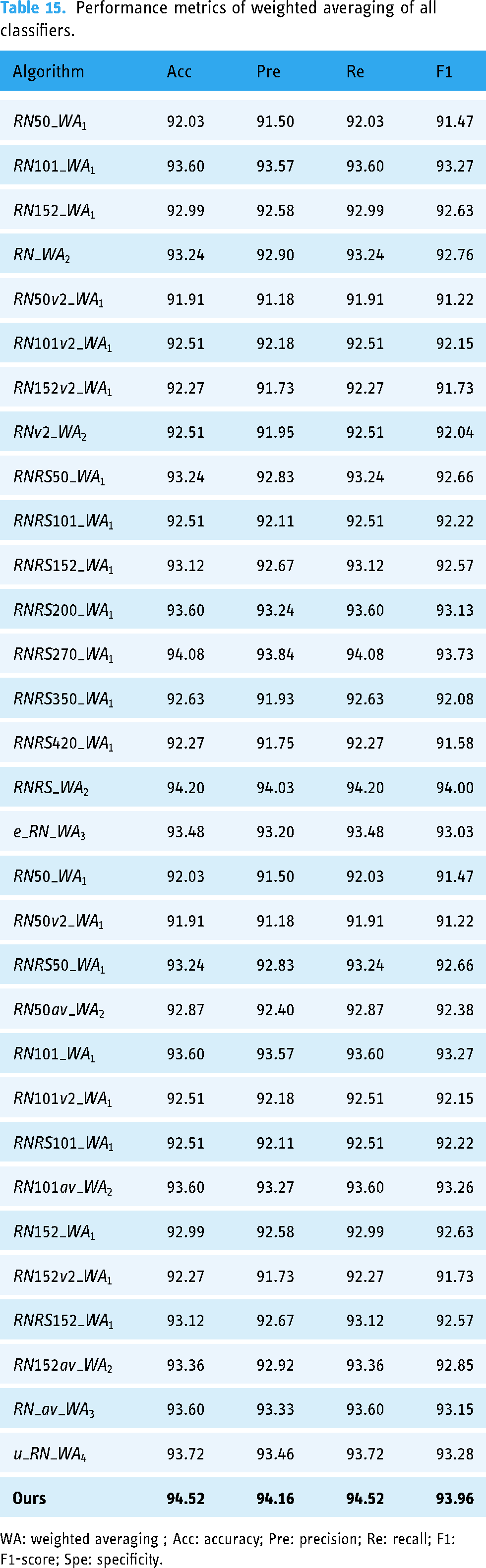
WA: weighted averaging ; Acc: accuracy; Pre: precision; Re: recall; F1: F1-score; Spe: specificity.
Table 15 compares the performance metrics of various classifiers using the WA technique at different levels with our IGIA approach. The results clearly showed that IGIA consistently outperformed WA across all levels and metrics, proving the superior effectiveness of our method. Boldface results denote the highest performance.
Regarding accuracy, the highest value achieved by the WA methods was 94.20%, observed with
Precision also favored IGIA. The highest precision among the WA methods was 94.03%, achieved by
Recall was another metric where IGIA excelled. The best recall for WA methods was 94.20% by
The F1-score further highlighted the superiority of IGIA. The highest F1-score among the WA methods was 94.00%, recorded by
In conclusion, our IGIA approach demonstrated superior performance across almost all evaluated metrics compared to the WA technique. By addressing the limitations inherent in WA, IGIA provided a more robust and effective ensemble method for classifier performance enhancement. This comprehensive improvement highlighted the potential of IGIA as a preferred method for classifier ensemble techniques.
Based on the comprehensive performance comparisons mentioned above, it is evident that our approach, integrating AT and IGIA, represented an optimal architecture compared to existing methods.
Answers to the research questions
Discussion and extended comparison
Our exploration of IGIA spanned four distinct levels, culminating in the attainment of optimal performance. Initially, we leveraged all variations of ResNet pre-trained models, including three variants of Base ResNet, three variants of ResNet version 2, and seven variants of ResNetRS. These were coupled with different CNN architectures, such as C_CNN, CA_CNN, SEA_CNN, and SA_CNN, resulting in 13 distinct classifiers. Each of these combinations underwent thorough evaluation at every level.
Similarly, as we progressed through subsequent levels of ensembling, we observed incremental improvements, yielding increasingly superior results. This progression validated the efficacy of our novel IGIA method.
Our ML-IGIA distinguished itself through its robustness, hierarchical approach, selective use of classifiers, and meticulous ensemble strategy, ultimately yielding superior outcomes. A comprehensive comparison provided in Table 16 underscores the significant advancement in results compared to previous research efforts. Despite employing a larger array of classifiers, our advanced yet user-friendly approach demonstrated clear superiority in overall performance, generalization, and evaluation metrics within this domain.
Comparison of our proposed model with other existing models (utilizing HAM10000 dataset with six classes).

HAM10000: Human Against Machines 10000; Acc: accuracy; Pre: precision; Re: recall; F1: F1-score; Spe: specificity; ML-IGIA: multi-leveled inverse Gini indexed averaging; CRV: customized ResNet variants.
Boldface results denote the highest performance.
Additionally, the comparison of our proposed architecture with existing state-of-the-art methods, demonstrated in Table 17, declares the superiority of our approach.
Comparison of our proposed model with state-of-the-art methods (utilizing HAM10000 dataset with six classes).

HAM10000: Human Against Machines 10000; Acc: accuracy; Pre: precision; Re: recall; F1: F1-score; Spe: specificity; ML-IGIA: multi-leveled inverse Gini indexed averaging; CRV: customized ResNet variants.
Boldface results denote the highest performance.
Threats to validity
Outlined below are certain aspects that could be identified as minor limitations within our study, presenting opportunities for further investigation and refinement:
The study is constrained by its reliance on a single dataset for both training and evaluation purposes. This constraint raised concerns regarding the generalizability of our model to diverse datasets with varying characteristics. Training a model solely on one dataset might have failed to encompass the full range of variations present in other sources, potentially resulting in diminished performance when applied to new and unseen data. While the inclusion of a diverse array of classifiers in the initial level could bolster the robustness of our model, it also introduced computational challenges. Employing numerous classifiers increased the computational complexity and resource demands during both the training and inference stages. This might have imposed limitations on the scalability of our approach, particularly when confronted with larger datasets or resource-constrained computing environments. These identified limitations underscored areas where our approach could benefit from further refinement and extension to effectively address potential challenges and enhance its overall performance and practical utility.
Conclusion and future work
In this study, we have developed a novel approach to skin lesion classification by leveraging CRV integrated with three attention mechanisms: CA, SA, and SEA. These attention-integrated ResNet variants are combined with a unique multi-level EL strategy, named inverse Gini indexed averaging (IGIA), and its multi-leveled variant (ML-IGIA). This innovative method addresses several challenges in the field of skin lesion classification, including class imbalance, optimal feature extraction, and the determination of optimal weights in ensemble models.
Our approach effectively balances the training dataset to ensure an unbiased evaluation of test and validation data. By incorporating attention mechanisms, we enhance the focus on crucial features within the input data, thereby improving the model’s ability to accurately classify skin lesions. The novel EL technique, IGIA, determines optimal weights for each ResNet variant, surpassing traditional methods and achieving superior performance. Specifically, our method achieved a remarkable accuracy of 94.52% on the HAM10000 dataset, demonstrating its effectiveness compared to existing approaches. Furthermore, to enhance the interpretability of our model, we have utilized Grad-CAM visualization. This technique allows the model to highlight specific regions relevant to diagnosed skin conditions, thereby improving transparency and providing valuable insights into the model’s decision-making process. For future work, we plan to extend our approach to additional skin lesion datasets, including ISIC2018, ISIC2019, ISIC2020, PH2, and PAD UFES 20. Additionally, we aim to develop a new dataset by collecting images from hospitals in Bangladesh, which we will then classify using our architecture. Furthermore, we intend to refine our methodology by experimenting with a reduced number of base classifiers and evaluating the performance of IGIA.
Footnotes
Acknowledgements
No specific acknowledgements.
Contributorship
Anwar Hossain Efat: conceptualization, data curation, formal analysis, methodology, software, and writing–original draft. SM Mahedy Hasan: conceptualization, formal analysis, supervision, and writing–review and editing. Md Palash Uddin: formal analysis, supervision, validation, and writing–review and editing. Faysal Hossain Emon: formal analysis, investigation, and writing–review and editing.
Ethical approval
This study involves the analysis of human skin disease data collected from a publicly available Harvard repository. The dataset is licensed under the Attribution-NonCommercial 4.0 International license. The data was carefully curated by Tschandl et al. (2018) and is used in accordance with the license.
Declaration of conflicting interests
The author(s) declared no potential conflicts of interest with respect to the research, authorship, and/or publication of this article.
Funding
The author(s) received no financial support for the research, authorship, and/or publication of this article.