Monkey king evolution (MKE)-GA-SVM model for subtype classification of breast cancer

Abstract

Objective

Recently, numerous research studies have concentrated on employing hybrid metaheuristic approaches for the analysis and diagnosis of breast cancer which motivated us to devise a computer-driven diagnostic tool that could aid in improving the precision of clinical decision-making.

Methods

In the present study, an integrated metaheuristic machine learning approach-based predictive model was developed that can classify breast cancer into subgroups using clinicopathological data acquired from tertiary care hospitals or oncological institutes.

Results

Monkey king evolution (MKE) was utilized to refine the hyperparameters of the support vector machine to achieve optimal settings, and genetic algorithm (GA) was used to choose the pertinent clinical and pathological attributes involved in classification before being applied to the support vector machine (SVM) classifier for prediction. A comparison was conducted between the results of the integrated MKE-GA-SVM model and those derived from conventional feature selection and hyperparameter tuning models such as GA-SVM, grid search-SVM, and SVM-recursive feature elimination (RFE). The effectiveness of the results was evaluated by applying the 10-fold cross-validation technique to the three multicentre datasets across all models. The integrated machine learning (ML) model achieved classification accuracies of 91.4%, 86.6%, and 75.5% across three clinicopathological breast cancer datasets, outperforming the existing models. The generated model performance was also assessed with notable metrics, namely F1-score, precision–recall curve, area under the ROC curve, mean square error and logarithmic loss.

Conclusion

Thus, the newly developed bio-inspired integrated metaheuristic model may be deployed as a surrogate diagnostic tool that allows clinicians to offer patients with better therapeutic outcomes.

Introduction

Breast cancer (BC), a prominently diagnosed cancer in women, originates from mutations in breast cells, causing irregular growth and the development of tissue masses referred to as tumours. According to breast cancer statistics 2022, ¹ around 287,850 cases were diagnosed with invasive breast cancer in the USA while there were 51,400 new cases that underwent treatment for ductal carcinoma in situ (DCIS) and 43,250 women lost their lives due to breast cancer. The diverse biological characteristics of breast cancer contribute to a range of histopathological features and clinical behaviours. Early detection of breast cancer and the implementation of intensive multimodal therapy have contributed to a notable decrease in the mortality rate associated with the disease. ² Prognosis in breast cancer is influenced by clinicopathological characteristics, including lymph node status and tumor size, as well as molecular biological aspects such as hormone receptors, human epidermal growth factor receptor 2 (HER2), and molecular subtype. ³ Hormone receptor testing is a well-established approach in standard clinical settings for managing breast cancer patients. ⁴

The categorization of breast cancer involves the use of immunohistochemistry staining for human epidermal growth factor receptor type 2 (HER2), progesterone receptor (PR), and oestrogen receptor (ER), which is widely known as a standard and accepted procedure.

Breast cancer is categorized into four primary subtypes – luminal A, luminal B, HER2-positive, and triple-negative breast cancer (TNBC) – determined by the expression levels of three hormone receptors. Luminal A subtype is characterized by low grade tumour, less likely to relapse, better prognosis and greater survival rate when compared with other breast cancer subtypes. It exhibits a favourable response to hormone therapy, especially tamoxifen and/or aromatase inhibitors, while offering limited advantages from chemotherapy. ⁵ Luminal B, when compared with luminal A grows more quickly, has a higher grade of tumour and a worse prognosis. Hormone therapy along with higher percentage of chemotherapy are the treatment modalities available for luminal B. ⁶ Herceptin or targeted therapy is effective in treating Her2-positive breast cancer that slows down the abnormal growth of HER2 protein and also has a greater response to chemotherapy schemes. ⁷ TNBC is an invasive subtype that possesses a high tumour grade, a poor prognosis, early recurrence development, distant metastases, and minimal therapy options. TNBCs exhibit distinctive morphological, molecular, and clinical characteristics.^8,9 Hormonal therapy and/or trastuzumab are ineffective for TNBC patients. However, the nature of these tumours makes them chemo sensitive. Surgery followed by chemotherapy is usually the treatment regimen supported for this particular kind of breast cancer. As of now, the US Food and Drug Administration (FDA) has not approved any particular therapy specifically targeting this devastating disease. ¹⁰ Thus, the clinical outcome, therapeutic responses, and patient survival rates of each of these subtypes are distinct. This entails the subgrouping of breast cancer into specific categories in order to plan effective treatments and offer accurate therapeutic options.

The support vector machine (SVM) serves as a robust machine learning (ML) method, particularly effective for categorization tasks, as it demonstrates proficiency in handling diverse medical datasets and revealing intricate relationships among them. Vapnik carried out the first research into the concept of a linear support vector machine in 1963. ¹¹ Finding the ideal hyperplane that linearly splits all the data points in two distinct areas is the primary goal of SVM, and this is done by maximizing the margin. Support vectors are points of data that are closest on both sides of the decision boundary, and the imaginary lines that run through them are referred to as margins. Margins are actually the regions where no data points lie. As a result, maximization of the margin width will produce the ideal hyperplane. When the ideal hyperplane is close to the data points, the margin will be smaller and the model will generalize well when used with training data, but not with unseen data. There are two types of margins: soft margin and hard margin. When the data can be separated into two distinct sets to avoid misclassification, SVM are trained with hard margins. When the data cannot be segregated exactly into two separate groups or when required a greater generality from the classifier, opting for a soft margin is preferred thereby allowing some misclassification. SVMs differ from other classification algorithms in that they maximize the distance between the closest points of data for all classes when selecting the decision boundary. SVMs can handle high-dimensional data and work well with small datasets, which is one of its main benefits. By employing a strategy referred to as the kernel trick, SVMs can also be utilized for non-linear classification. The input data undergo mapping through the kernel method, transitioning into a higher-dimensional space and enabling them to be linearly separated. The selection of the kernel, however, can affect SVM performance, and large datasets can make them computationally expensive. Successful application of SVM has been reported in numerous literature studies, including breast cancer prognosis, cancer genomics, developing recurrence predictive model, breast cancer classification and survival analysis. Ferroni et al. ¹² constructed a prognostic predictive model by integrating random optimization (RO) with SVM. This approach aimed to extract prognostic information from the demographic, clinical, and biochemical data routinely collected from breast cancer patients. Huang et al.’s ¹³ investigation on the categorization capability of SVMs concerning cancer genomics had led to the evolution of new biomarkers, targeted treatments, and significant understanding of cancer-driver genes. Kim et al. ¹⁴ established a unique prognostic model utilizing SVM for predicting BC recurrence rate 5 years post surgery in a cohort of Korean individuals. The predictive performance of the model was additionally assessed and compared with other pre-existing models in use. Wu et al. ¹⁵ highlight the efficacy of SVM in discriminating triple-negative breast cancer from non-TNBC. They achieved this by analysing RNA-sequence data gathered from two distinct patient datasets, showcasing SVM’s potential in this diagnostic context. Leveraging clinical factors centred on tumours, such as size, age at diagnosis, and stage, Mihaylov et al. ¹⁶ estimated the breast cancer patient's survival duration. The outcomes demonstrated the merits of linear SVM as well as other models in survival analysis. Bai et al. ¹⁷ elucidated the contribution of peripheral lymphocytes in identifying prognostic biomarkers. Furthermore, their goal is to establish SVM as a robust predictor of prognosis for patients with breast cancer. A set of SVM parameters influence the behaviour of a ML model that are not used during the model training phase. These parameters, also referred to as hyperparameters, must be changed beforehand, prior to the training phase. A learning algorithm determines the model parameters for the current data set, then keeps updating these values as it learns. These parameters are incorporated into the model once learning is complete. The hyperparameters are algorithm specific and used to calculate the model parameters. The hyperparameter tuning procedure comprises discovering a set of ideal hyperparameter values for the learning algorithm and then using this improved algorithm on each given data set. The kernel is the primary hyperparameter for the SVM. The partitioning of the classes in classification and the effectiveness of the method are significantly influenced by the kernel choice and their hyperparameters. The concept of a soft margin, which focuses on maximizing the correct classification of data points during training, delineates the decision boundary in an optimization problem by increasing the separation between the decision border and the support vectors. The C parameter manages this trade-off. The C parameter imposes a penalty to each incorrectly categorized data point. A lower value of C entails choosing a decision boundary with a broader margin, but this decision comes with the trade-off of increased misclassifications since the penalty for inaccurately classified points is kept minimal. With a large value for C, SVM generates a decision boundary featuring a narrower margin, as it endeavours to minimize the number of misclassified samples by imposing a substantial penalty. In the setting of SVM with radial basis function (RBF), the RBF's gamma value governs the scope of influence caused by a single training point. Low gamma values suggest a wide similarity radius, which causes more points to be grouped together. The points must be relatively close to one another for high gamma values for them to be included in the same class. Due to this, models with extremely high gamma values tend to be overfit. As a result, determining the hyperparameters’ optimal value remains always challenging. In this paper, MKE algorithm has been deployed to optimize the SVM hyperparameter's values for SVM classifier to be used for prediction.

The practice of selecting a subset of pertinent features (predictors and variables) to be used in the creation of a model is known as feature selection in ML. If the proper subset of features is selected, feature selection can minimize the ML model’s complexity and simultaneously increase the model’s accuracy. Further, it makes the ML algorithm's training process faster and decreases overfitting. Feature selection also decreases the dimensionality and enhances the output attribute vector's quality by deleting extraneous and inaccurate features.^18–20 Feature selection has been utilized for many applications, namely cancer classification, specifically to help with breast cancer and diabetes diagnosis, ²¹ gait analysis, ²² text mining, ²³ gene prediction, ²⁴ glaucoma prediction,^25,26 speech recognition, ²⁷ etc. From a taxonomic viewpoint, feature selection methods can be classified into filter, wrapper, and embedded approaches,^28,29 each representing distinct strategies in the selection process. Usually, filter methods are utilized as an initial preprocessing step. The filter method chooses features using statistical measures and is suitable for datasets with a smaller number of features. Additionally, it generally demands low computational skills for performance. Filtering techniques frequently fail to appropriately recognize the samples during the learning phase as the link between classifiers and characteristics is not taken into account. It is computationally more efficient to employ filter methods while working with high-dimensional data. A filtering strategy inhibits data overfitting and is devoid of any ML algorithm. Wrappers necessitate a process of exploring all conceivable feature subsets, assessing the quality of each subset through training, and the performance of the classifier is evaluated utilizing each subset. It employs a greedy search strategy by comparing every potential feature combination to the evaluation criterion. Wrappers strive to train a suitable ML algorithm using only a subset of the necessary features to gauge the effectiveness of the training model. Evaluating the accuracy achieved in each of the preceding stages, a wrapper algorithm contemplates whether to include or exclude a feature from the chosen set of features. Wrapper methods are commonly more resource intensive and computationally demanding in comparison to the majority of the filtering approaches. The drawbacks in traditional wrapper approaches ³⁰ include the recursive evaluation of the chosen feature vector, which leaves out some features from the initial assessment. Additionally, because the user specifies the arguments, some feature combinations may not be considered even with more exactness. These problems could lead to overfitting and overhead in the search process. Evolutionary wrapper methods have effectively overcome the drawbacks associated with traditional wrapper techniques, gaining prominence, particularly in situations characterized by expansive search areas. Multiple potential solutions to a problem can be solved using evolutionary optimization approaches, which are population-based metaheuristic methods described by a group of people. The feature vector is represented by each entity of the feature selection tasks. Every candidate solution is evaluated and assessed for consistency using an objective or target function. To generate new entities capable of producing the next generation, ³¹ the selected individuals are exposed to genetic operators’ involvement. In the broad field of evolutionary algorithms, genetic algorithms (GAs) exemplify evolutionary heuristic search methods, drawing inspiration from Darwin's theory of selection and genetics as their foundational principles. Gas^32–35 carry out search in complicated, vast, and multimodal settings, yielding solutions that closely approximate optimality for the objective or fitness function in optimization problems. An individual's identity is defined by a set of characteristics referred to as genes, which collectively constitute a sequence, giving rise to chromosomes. The collection of all such chromosomes forms a population. The fitness function aids in determining the population's overall level of fitness. Every individual is provided with a fitness score, which also impacts their likelihood of being selected for reproduction. The probability of being considered for reproduction increases with increasing fitness scores. During the selection phase, individuals are chosen to produce offspring through reproduction. The entire group of individuals selected is subsequently set in pairs of two to maximize reproduction. To produce new offspring, the genetic algorithm utilizes two variation operators – namely crossover and mutation – applied to the parent population. The steps of selection, crossover, and mutation endure for a predetermined number of iterations or until the termination criterion is fulfilled. This study utilizes the GA’s feature selection capabilities to the SVM model to choose potential features for model training.

This research presents a hybridized monkey king evolution (MKE)-GA-SVM model for breast cancer classification employing clinical, pathological, and demographic data gathered across three specialized cancer care hospitals/oncological centres. A more robust and improved iteration of the ebb-tide-fish algorithm, known as the monkey king evolutionary (MKE) algorithm, ³⁶ was initially introduced in 2016 for global optimization. Due to its faster convergence and accuracy along with identical time complexity as compared to PSO variations, the MKE method has been employed in this paper to identify the optimal settings of SVM hyperparameters. The values of the SVM hyperparameters kernel, C, and gamma are taken into account for optimal conditions. Various kernel functions like radial basis, sigmoid, linear, and polynomial, and an array of evenly spaced range of C and gamma values in the logarithmic scale have been presented as options in this study and implemented in Python with MKE algorithm to achieve the optimal SVM hyperparameter combination. As a result, the most suitable kernel function and optimized C, gamma values can be automatically evolved into an SVM hyperparameter combination. The concepts of natural genetics and evolution serve as the foundation for GA, which are stochastic search and optimization approaches with significant latent parallelism. Search is carried out by GAs in complicated, vast, and multimodal landscapes and they get improved over time. GAs demonstrate their ability to identify the most pertinent features for classification tasks by selecting a specific subset from the feature pool. This chosen subgroup, characterized by higher fitness scores, is then incorporated into the model training process. But before applying GA to the SVM estimator, it is crucial to figure out the number of chromosomes required for the initial population, maximum feature subset size, crossover and mutation rate, and number of generations to recur genetic selection. Thereafter, the tuned SVM estimators are used for the training phase and subsequent classification of breast cancer patients into two different classes. The results obtained from the integrated MKE-GA-SVM model underwent analysis and were compared with outcomes of traditional feature selection and hyperparameter tuning methods, such as GA-SVM, grid search-SVM, and the SVM-recursive feature elimination (RFE) model. To validate the results across three multi-centre datasets, all models underwent a 10-fold cross-validation technique. The integrated ML model produced classification results that were superior to those of the other conventional models when implemented on three clinicopathological datasets pertaining to breast cancer. The generated model performance was also assessed with notable metrics, namely mean square error (MSE), logarithmic loss (Log Loss), F1-score, area under the ROC Curve (AUROC), and the precision–recall curve (PR curve).

The rest of the sections of this article are structured as follows: The next section focuses on the datasets utilized in this analysis, along with conventional ML feature selection and hyperparameter tuning models and the proposed model. We then explore the performance of the integrated MKE-GA-SVM model, drawing comparisons with established feature selection and hyperparameter tuning techniques. It also encompasses a statistical analysis illustrating how clinicopathological factors influence the identification of TNBC/non-TNBC cases and recurrence/no-recurrence events. This is followed by an in-depth discussion, while the last section concludes the paper.

Methods

Datasets

The BioStudies database, ³⁷ developed by the European Bioinformatics Institute (EMBL-EBI), is designed to store data from a diverse array of biological studies. Researchers utilize BioStudies to deposit data associated with publications or projects, ensuring a stable and accessible repository. It serves as a valuable resource for ensuring that data are available for future reference and for use by other researchers in the scientific community. The current analysis involves three datasets: two datasets of patients with breast cancer diagnosis from African nations were retrieved from the Biostudies database, while the third breast cancer dataset was sourced from the UC Irvine Machine Learning Repository. The two African datasets collected from the biostudies were made publicly available as a CSV file since anonymous patient identities were supplied by the authors of the original research as a supplementary file, along with their respective publications in Biostudies. Thus, the freely available datasets sourced from the original research has been utilized for conducting this secondary analysis. The first study of the original research was conducted retrospectively, involved a cohort of 905 patients who had undergone treatment for breast cancer. This research initiative commenced in 2009 at the National Institute of Oncology in Rahat, Morocco, and extended its duration until 2014. ³⁸ Every patient's medical file was thoroughly examined to gain insights about their clinical, pathological, and therapeutic aspects. 405 cases in total were eliminated owing to insufficient data, foreign nationals, and male patients. Rest of the 500 malignancy cases were separated into two groups: 85 cases of TNBC and 415 cases of non-TNBC based on their molecular subtypes. ³⁹ Additionally, the clinicopathological characteristics, the pathogenic data needed for SBR grading, the prognosis, and therapy of TNBC patients were examined. Another prospective, non-interventional investigation ⁴⁰ of 251 patients histologically confirmed with tumour staging was carried out at the radiotherapy department of the Lagos University Teaching hospital in Nigeria. This original study encompassed female patients over the age of 18 who had received treatment between July 2017 and July 2019 at the outpatient clinic. The individual patients were interviewed about their socio-demographics and complications by means of a structured proforma. The patients were allocated into two groups based on their molecular subtypes: 119 individuals, that is, 47.4% were categorized with TNBC, with the rest 43.2% classified as non-TNBC. The hospital dataset is easily accessible at Biostudies. ⁴¹ The third breast cancer dataset ⁴² was accumulated from the University Medical Centre, Institute of Oncology, Ljubljana, Yugoslavia, consisting of clinicopathological factors that influence the occurrence of recurrence/non-recurrence events. The dataset bears multivariate characteristics and comprises 286 cases that are individually described by nine clinical, pathological, and demographic factors, most of which are categorical. The pertinent authors of the primary research were consulted for ethical clearance to conduct this current secondary analysis. Given that the initial research was previously completed and published, repeated ethical approval was not essential.

Traditional feature selection and hyperparameter tuning ML models

Feature selection deals with choosing a selected number of pertinent features by eliminating unnecessary, irrelevant, or noisy features from the original set. To develop a predictive model, the feature selection procedure involves minimizing the amount of input variables. In other words, the main objective is to determine which features have the greatest influence on the predictive model. Furthermore, deleting less significant features that undermine the model to anticipate the targeted variables can lower overfitting and improve the model's generalization capabilities.

Recursive feature elimination, ⁴³ often known as RFE feature selection, a wrapper approach to feature selection lowers the model complexity by selecting important features and eliminating the less important ones. Recursive feature elimination works by ranking each feature's importance using the selected RFE ML technique, eliminating the lowest relevant feature, and then creating a model with the remaining attributes until the targeted number of features is reached. The algorithm updates the model using the remaining features after removing the least significant features in each iteration. RFE can be deployed in combination with any supervised learning technique, although SVM is the most common pairing. SVM-RFE is an SVM-based feature selection technique that utilizes SVM's classification power at its core and RFE wrapped around it to offer the most desirable combination of features for the best model performance. RFE is better suited for complicated data sets than other feature selection techniques because it takes feature interactions into account. The details about GA and SVM were covered in the preceding section. In classification setting, the feature selection capabilities of GAs can be employed to identify a subset of features with the highest fitness score, which can then be utilized in model training. GA has been used to determine the potential features for the SVM model in the training phase. But before using GA on the SVM estimator, it is crucial to set the size of chromosomes for the initial population, crossover rate, mutation rate, tournament size, and iterations. To obtain a more credible performance of the suggested model, 10-fold cross-validation procedures were applied. The benefit of using GA is that it performs an exhaustive search of the feature space using different sets of solutions that can improve over time. Because of the evolutionary approach, the subsets of variables identified by GAs are often more efficient than other feature selection approaches. The prediction accuracy as well as different model performance indicators may be enhanced by using the GA-SVM hybrid model to categorize various breast cancer variants. Grid search ⁴⁴ is a popular method of hyperparameter tuning that can make it easier to create and assess models for all possible combinations of algorithmic parameters per grid. Grid search involves creating discrete grids out of the hyperparameter domain. Cross-validation metrics are used to assess each set of grid values. The grid point is the best hyperparametric value combination that maximizes the cross-validation mean value. Grid-search is used to fine-tune the SVM hyperparameter values in the Grid-search SVM model. The hyperparameter settings are used to build the model, and prediction accuracy is assessed. The set of hyperparameter values that yields the highest model accuracy is then chosen for the training phase. The fine-tuned SVM estimator is then used to classify multiple variants of breast cancer. The suggested model was compared with the hybrid Grid search-SVM model.

The proposed model

The actions of the Monkey King, a character in the well-known Chinese legendary classic Journey to the West, served as the model for the MKE algorithm. The story follows the incredible exploits of the monk Sanzang and his three disciples as they journey to the west in quest of Buddhist sutras, with the Monkey King standing out as the most adept disciple. When the king of monkeys is in crisis, he may turn to several small monkeys to handle the difficult challenge, and every small monkey can provide feedback on a solution for the monkey king to choose from. Analogous to the ebb-tide-fish algorithm, ⁴⁵ the MKE algorithm comprises only a limited number of particles designated as monkey king particles.

To ascertain the quantity of monkey king particles within the population, we utilize a population rate denoted as R. The population size is indicated by PopSize, and the monkey king identities get initialized randomly with a sum equal to R*PopSize. Every monkey king particle within the population undergoes a transformation into a small cluster of monkeys to facilitate exploitation, while the remaining particles are employed for exploration as part of the evolutionary process. The R*PopSize particles in the population are then randomly chosen to have their labels changed to represent the fresh monkey king particles once every monkey king particle has been exploited. In the MKE technique, a monkey king particle turns into C × D smaller monkeys, where C acts as a constant and D denotes dimensionality. Although it often increases computing complexity, a higher C value indicates that the monkey king particle exploits the local area more and demonstrates superior performance on multimodal functions. The i-th small monkey particle within the group of C × D small monkeys is denoted as X_sm(i) in equation (2). All of these ‘small monkey’ elements possess identical values as X_MK,G (a monkey king particle of the Gth generation). The ‘small monkey’ components follow the evolution shown in equation (1) to search the area around X_MK,G, and X_MK,G changes to X_MK,G+1, when the chosen optimal value is derived from C × D ‘small monkey’ particles. The ordinary particle evolves according to equation (3). The term ‘X_{k,p best}’ refers to the historical best of the kth particle in the population, and ‘F’ stands for the direction vector's fluctuation coefficient, that is, the vector connecting the current location to the global best position.

$$X_{sm}(i)=\{x_1,x_2,\dots .,..x_j,\dots ..,x_D\}$$

$$x_j\to x_j\pm 0.2*\mathrm{rand}()*x_j,j\in \mathrm{D}$$

(1)

$$X_{MK,G+1}=\begin{array}{c}opt\\ i\in C\times D\end{array}\{X_{sm}(1),\dots \dots \dots .,X_{sm}(i),\dots \dots .,X_{sm}(C\times D)\}$$

(2)

$$X_{k,G+1}=X_{k,pbest}+F*rand()*(X_{gbest}-X_{k,G})$$

(3)

The proportional rate R is relatively small since the monkey king population particles serves as the perturbing components to improve optimization outcomes in less time. The key advantage of the MKE algorithm lies in its ability to incorporate a large-scale optimization feature, allowing for the effective resolution of challenges associated with large-scale optimization. It is easily parallelizable on distributed computing systems, enhancing computational speed. In the population-based differential evolutionary method known as MKE, the control parameter and the single evolution strategy have an impact on convergence and the exploration–exploitation ratio. This compelled us to apply the MKE approach to identify the most appropriate SVM hyperparameter settings. The values of the SVM hyperparameters kernel, C, and gamma are taken into account for optimal conditions. Various kernel functions like radial basis, sigmoid, linear, and polynomial, and an array of evenly spaced range of C and gamma values in the logarithmic scale have been presented as options in this study and implemented in Python 3.9.12 with the MKE algorithm to achieve the optimal SVM hyperparameter combination. As a result, the most suitable kernel function and optimize C, gamma values can be automatically evolved into an SVM hyperparameter combinations. However, it is essential to set the parameter values for population size, fluctuation coefficient, population rate, the quantity of new particles generated by the monkey king particle, and the scaling factor for monkey king particles before fitting MKE for SVM hyperparameter tuning.

$$\mathrm{population}\mathrm{\_}\mathrm{size}=40$$

$$\mathrm{fluctuation}\mathrm{\_}\mathrm{coeff}=0.7$$

$$\mathrm{population}\mathrm{\_}\mathrm{rate}=0.3$$

$$\mathrm{c}=3$$

$$\mathrm{fc}=0.5$$

where population_size = the population size of the particles, fluctuation_coeff stands for the direction vector's fluctuation coefficient, population_rate = percentage of new particles that monkey king particles produce and its value lies between 0 and 1, c represents the number of new particles generated by the monkey king particle, and fc denotes the scaling factor for monkey king particles.

The capability of GA to identify the most relevant features for classification problems is performed by choosing a specific subgroup of features from the feature pool that exhibits higher fitness scores. The fitness function analyses every individual's fitness score and uses that information to determine which individuals have the best chance of being selected for the next generation. Search is carried out by GAs in complicated, vast, and multimodal landscapes, and they get improved over time. GA has been used in this study to select potential features of SVM model that can take part in the training phase. But before applying GA to SVM estimator, it is crucial to figure out the number of chromosomes required for initial population, maximum feature subset size, crossover and mutation rate, and number of generations to recur genetic selection. The entire genetic procedure was carried out using statistical packages included in the Python 3.9.12 programming language.

$$\mathrm{estimator}=\mathrm{SVC}$$

$$\mathrm{cv}=10,$$

$$\mathrm{verbose}=1,$$

$$\mathrm{scoring}=\mathrm{accuracy}.$$

$$\max \mathrm{\_}\mathrm{features}=5,$$

$$\mathrm{n}\mathrm{\_}\mathrm{population}=20,$$

$$\mathrm{crossover}\mathrm{\_}\mathrm{proba}=0.5,$$

$$\mathrm{mutation}\mathrm{\_}\mathrm{proba}=0.2,$$

$$\mathrm{n}\mathrm{\_}\mathrm{generations}=20,$$

$$\mathrm{crossover}\mathrm{\_}\mathrm{independent}\mathrm{\_}\mathrm{proba}=0.5,$$

$$\mathrm{mutation}\mathrm{\_}\mathrm{independent}\mathrm{\_}\mathrm{proba}=0.05,$$

$$\mathrm{tournament}\mathrm{\_}\mathrm{size}=3,$$

$$\mathrm{n}\mathrm{\_}\mathrm{gen}\mathrm{\_}\mathrm{no}\mathrm{\_}\mathrm{change}=10,$$

$$\mathrm{caching}=\mathrm{True},$$

$$\mathrm{n}\mathrm{\_}\mathrm{jobs}=\text{-}1$$

where SVC = SVM classifier, cv = 10 signifies 10-fold cross-validation, verbose = controls the output's verbosity, scoring = ‘accuracy’ implies that every individual of the initial population is assigned a score in accordance of the targeted metrics, max_features = maximum features chosen for the starting population, n_population = population size employed by the genetic algorithm, crossover_proba = the chance of genetic material being transferred from one generation to the next through parent–child cross-over, mutation_proba = the likelihood that a random mutation will occur within the features, n_generations = how many generations must be repeated for genetic selection, crossover_independent_proba = the possibility that an individual trait will be picked for cross-over and create a child in the next generation, mutation_independent_proba = the chance that an independent feature will be mutated for the next genetic evolution, tournament_size = the number of top-performing individuals selected based on scoring metrics for participation in the tournament, n_gen_no_change = the termination of optimization occurs after a specified number of iterations if there is no change in the value of the best individual, caching = for True value, the scores of best individual in every generation is cached, and n_jobs = number of parallel-running cores. The default value is 1, and if it is set to −1, the number of jobs equals the number of cores.

Pandas, a freely available Python toolkit, is utilized for efficiently and easily managing relational or labelled data. It provides a variety of data structures and processes for working with both numerical and time series data. Pandas’ data frame resembles a feature matrix, with rows denoting the anonymous identity of patients and columns signifying the sociodemographic, clinical, and pathological parameters of corresponding patients.

The open-source Python library, Numeric Python (NumPy), was imported to perform computations and process elements of multidimensional and linear arrays. Scikit-Learn, ⁴⁶ a built-in python toolkit for ML, has been employed to deliver a range of data analysis components like data preprocessing, model fitting, model selection, model evaluation, cross validation, and visualization. Importing libraries, loading data into Pandas, managing missing value and categorial features, feature scaling, normalizing the data set, and lastly dividing the data set into training and test sets were the steps that were carried out for data processing in Python. The SimpleImputer function was used to impute missing data using multiple imputation approaches such as mean, median, most_frequent across each column, or by assigning a constant value. A function named StandardScaler was utilized for data standardization, aiming to resize the distribution of values. This process ensures that the observed values have a mean of zero and a variance of one. The division of datasets into training and test sets was performed randomly using the train_test_split function. In this unified model, the train_test_split method randomly partitions the datasets in a 7:3 ratio, allocating 70% of the dataset for training and using the remaining 30% as a test set. The training dataset was employed to train the model, enabling it to learn from known data. Following the model's training on the training dataset, it is necessary to evaluate its performance using the test dataset. This dataset evaluates the model's performance and ensures that it can properly generalize to new or unseen data. A particular subset of the training set, denoted as the validation set, was utilized to evaluate the model's performance and fine-tune its hyperparameters. The SVM hyperparameters that has been taken into account for optimal setting are kernel, C, and gamma values. Various kernel functions like radial basis, sigmoid, linear, and polynomial, and an array of evenly spaced range of C and gamma values in the logarithmic scale have been presented as a sequence of parameter values in the form of a dictionary with parameters kernel, C, and Gamma so as to create a grid of parameters from which the MKE algorithm has to select the right combination. The hyperparameter tuned SVM model was then employed with GA to choose prospective clinicopathological features for model training. Feature selection is the process of selecting the most relevant features and eliminating the superfluous or irrelevant ones in order to improve the ML model's predicting abilities. Svclassifier is an estimator object that can fit the model with training data and perform classification from new data. Thus, the integrated model has been developed by considering two crucial steps of the model-building process – hyperparameter tuning and feature selection so as to enhance the model's interpretability and performance. A flowchart of the MKE-GA-SVM integrated model development method is delineated in Table 1.

Table 1.

Flowchart of the proposed MKE-GA-SVM integrated model.

The following are the necessary algorithm stages for the proposed MKE-GA-SVM prediction model whose actual implementation was performed in python:

Step1: Import the dataset as a data frame in pandas with rows = patient identity and the columns = the related patients’ sociodemographic, clinical and pathological parameters.

Step 2: Data standardization and missing value manipulation with SimpleImputer and StandardScaler functions.

Step 3: Class labels as (m × 1) targeted array.

Step 4: train_test_split () function for training and test datasets in the ratio of 7 : 3.

Step 5: Import MKE algorithm with set_parameters

Step 6: Choose the best kernel = : [“rbf,” “sigmoid,” “linear”, “poly”], C and gamma values using MKE algorithm.

Step 7: Print best_params_

Step 8: Genetic selection with estimator = SVC and best_params_

Step 9: Display feature selector support_.

Step 10: Calculate scoring = “accuracy.”

Research ethics and patient consent

The present analysis includes three datasets: two datasets of individuals with breast cancer from African countries namely Morocco and Nigeria were obtained from Biostudies, and a third breast cancer-related dataset sourced from the UC Irvine Machine Learning Repository. The datasets analysed in this paper comprises of retrospective data from patients treated for breast cancer. Each of these original studies obtained ethical approval from their respective institutional ethics board, and the authors have provided anonymous patient datasets as a supplementary material. The corresponding authors of the original research were informed for conducting this secondary analysis. Ethical clearance was not required since the original research had already been conducted and published in 2020. For investigations involving the same publicly accessible data, recurrent ethical consent was not necessary. Furthermore, human participants were not directly involved in this secondary study. Accordingly, the patients’ informed consent was not required to conduct the present research. The third dataset has been gathered from UCI ML repository that maintains several datasets to serve the ML community publicly. For the sake of conducting the current investigation, the datasets acquired were carefully examined and validated with the clinical partners.

Results

This study examines datasets from three tertiary care hospitals or oncological facilities that include patients who presented with breast cancer and bears certain clinicopathological characteristics. The first dataset encompassed 905 individuals who had received medical care for breast cancer at the National Institute of Oncology in Morocco. Eventually, 500 cases were taken into account for study after excluding patients with missing medical data, international and male patients. The second dataset included assessments conducted on 251 breast cancer patients who were registered at the Lagos University Teaching Hospital in Nigeria. The University Medical Centre, Institute of Oncology, Ljubljana, Yugoslavia, provided the third breast cancer dataset of 286 cases, which included clinicopathological variables influencing the likelihood of recurrence/non-recurrence events.

Performance evaluation of MKE-GA-SVM integrated model

The MKE-GA-SVM model underwent performance evaluation using noteworthy metrics, namely mean square error (MSE), logarithmic loss (Log Loss), F1-score, area under the ROC curve (AUROC), and precision–recall curve (PR curve). A tabular matrix of size N × N, known as a confusion matrix, is employed to gauge the efficacy of a predictive model, where N is the total number of classes to be classified. A confusion matrix presents the counts of correct and incorrect predictions made by a classifier. The efficiency of the integrated model is assessed by the confusion matrix, which calculates performance metrics including accuracy, precision, recall, and F1-score. For the sake of simplicity, the datasets from the Lagos University Teaching Hospital in Nigeria, National Institute of Oncology in Morocco, and the University Medical Centre in Yugoslavia were labelled as datasets 1, 2, and 3, respectively. Instances of TNBC and non-TNBC were labelled as 1 and 0, respectively. Figure 1 displays the classification report of the MKE-GA-SVM model on datasets 1, 2, and 3. This report illustrates the precision, recall, F1-score, and support metrics for the trained integrated MKE-GA-SVM model. The integrated model identifies TNBC and non-TNBC participants with higher accuracy rate, as seen by higher values of key performance criterions across the three datasets. The efficiency of the binary classification model is graphically depicted by the AUC-ROC curve, an assessment tool for classification across various threshold levels. AUC, which stands for the degree or measure of separability, is represented by ROC (receiver operator characteristic), which illustrates a probability curve. The ROC curve is visually depicted, plotting the false-positive rate (FPR) on the X-axis and the true positive rate (TPR) on the Y-axis, encompassing various threshold values ranging from 0 to 1. A higher X-axis value on a ROC curve denotes more false-positive cases as compared to true negatives. A higher value on the Y-axis, however, signifies a greater proportion of true positives relative to false negatives. The ability to strike a balance between false-positives and false-negatives will thus play a pivotal role in determining the choice of the threshold. An AUC of 1 indicates the classifier's ability to accurately distinguish all classes, while an AUC of 0 suggests that it will assign either a specific class or a random class to each instance. There is a good possibility that the classifier will separate all the instances of the two classes when 0.5 < AUC < 1. This is because the classifier can recognize a higher number of true positives and true negatives compared to false negatives and false positives. By analogy, with elevated AUC values, the model demonstrates increased effectiveness in distinguishing between patients with TNBC and those without TNBC. In the ROC curve, the point (0.5, 0.5) represents a model with no skill. A line slanting from the bottom left to the top right of the plot represents a model with no skill at each threshold and has an AUC value of 0.5. A model is considered to have perfect skill when it is plotted with a line that runs from the bottom left to the top left to the top right of the curve and lies between (0, 1). ⁴⁷ The integrated model's ROC curve on three different datasets is displayed in Figure 2. With an FPR value of 0.1, the ROC curve of dataset 1 achieved sensitivity = 1 and covers a substantial area prior to crossing the no-skill line. The ROC from dataset 2 reached the highest sensitivity value of 0.9 with a corresponding fall-out of 0.5 before touching the no-skill line. However, dataset 3's ROC curve occupies certain area above the diagonal line within a fall out value = 0.4 and then moves below the no-skill line up to FPR of 0.9 before finally moving upwards to collide with (1,1).

Figure 1.

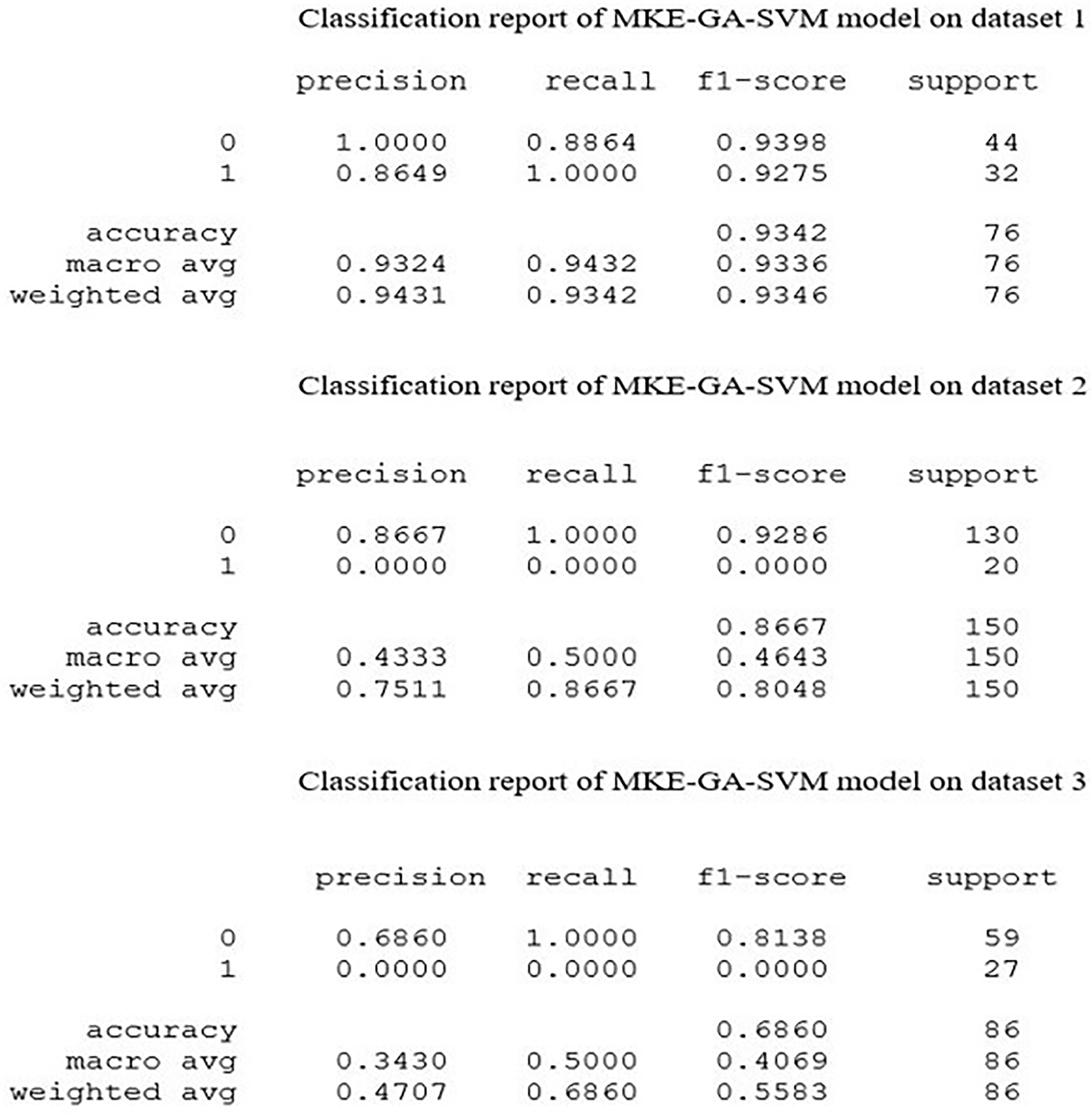
Classification report of MKE-GA-SVM integrated model on three datasets. 0 stands for non-TNBC cases and 1 represents TNBC cases.

Figure 2.

Area under the ROC curve (AUROC) of MKE-GA-SVM integrated model on three datasets. AUROC is plotted graphically with false positive rate on the X-axis and true positive rate on the Y-axis. The blue dashed line denotes the no-skill line. The orange colour line represents the model skill before reaching (1,1).

The widely used loss function, known as the MSE, computes the sum of the squares of the variations between the estimated and actual values produced by the model, divided by the overall count of patients included in the dataset as test cases.

$$MSE={\displaystyle \frac{1}{N}{\sum }_{I=1}^N(y_i-\widehat{y_i}{)}^2}$$

(4)

where y_i represents the model estimated value, $\widehat{y_i}$ denotes the actual value, and N represents the total count of patients across the three datasets utilized as test cases. The MSE is zero if the model is error free. As the model error increases, so does its value. Lower MSE values suggest that the predicted and actual values are close. The error squares prevent MSE from being negative. The MKE-GA-SVM model exhibited MSE values of 0.065, 0.133, and 0.31 for datasets 1, 2, and 3, respectively. These outcomes demonstrate decreased MSE values and a high degree of integrated model classification performance.

In assessing the efficacy of the classification model that relies on the probability concept, logarithmic loss, commonly known as Log Loss, is employed as a pertinent evaluation metric. It establishes how effective a model is by measuring the variation between the expected probability and the actual values. Log Loss quantifies the range to which the prediction probability matches with the associated actual or true value and thereby increasing the penalty value for incorrect predictions. When comparing models, Log Loss statistics can be a valuable tool even though they are hard to understand. A lower Log Loss value corresponds to better model predictions. The computation of Log Loss is performed by multiplying the negative average with the sum of the logarithmic estimated probabilities for every patient.

$$Loglos{s}_i=-[y_{i}ln{p}_i+(1-y_i)ln(1-p_i)]$$

(5)

where i refers for a specific patient, y_i represents the actual value, p_i denotes the predicted probability, and log stands for the number's logarithmic value. The Log Loss value obtained from dataset 1, 2, and 3 were 0.85, 0.38, and 0.69 respectively.

The effectiveness of a classifier at several probabilistic thresholds is depicted graphically by precision–recall curves. At varying probability thresholds, the precision–recall curve identifies the balance between the TPR (recall) and positive predictive value (precision), providing valuable insights into the model's performance. The functionality of binary classification methods is assessed using the precision–recall curve, particularly when classes are highly imbalanced and provide more information than the ROC plots. Precision–recall curves are plotted with recall and precision on the X- and Y-axes, respectively, at various threshold settings. A low FPR corresponds to high precision, and a low false negative rate implies high recall. A wide AUC indicates high recall and precision. When plotted, it frequently takes a zigzag route that moves up and down. Typically, a precision–recall curve with no overlapping output denotes a higher degree of performance than one near the baseline. Figure 3 shows the integrated model's precision–recall curve for three datasets. The precision–recall curve for dataset 1 is significantly higher than the baseline, with no overlapping regions. The dataset 2's precision–recall curve initially falls below the baseline with recall value 0.0 and then moves upward to follow zigzag route before coinciding with the baseline. Dataset 3's curve was initially high, but it eventually descended below the baseline from recall value 0.5 and finally touched it at recall value 1.

Figure 3.

Precision–recall curves of MKE-GA-SVM integrated model on three datasets. It is plotted graphically with recall on the X-axis and precision on the Y-axis. The blue dashed line denotes the no-skill line just above the base and the orange colour line represents the model skill before touching the baseline.

Convergence is the stopping criterion for an optimization ML algorithm when the algorithm reaches a stable point after which subsequent iterations fails to significantly enhance the results. Learning curves are used to quantify and empirically investigate the convergence of an optimization process. Learning curves are an often-used diagnostic tool in ML for algorithms that gain knowledge incrementally from a training dataset. To fit our model with an optimal bias-variance trade-off, the learning curve can be helpful in determining the quantity of training data to use. Learning curve plots indicate how learning performance with respect to experience changes over time. One can identify an underfit, well-fit, or overfit model employing learning curves on training and validation datasets for model performance.

Figure 4 illustrates the learning curves for datasets 1, 2, and 3 by plotting the training set size on the X-axis and the corresponding accuracy score on the Y-axis. The cross-validation score in dataset 1's learning curve began low and gradually increased as the size of the training set became larger, whereas the training score was initially high and became almost steady with a training set size above 175. For dataset 2, the cross-validation score nearly stays constant as the training sample size increases, but the training score rapidly drops between 100 and 275 training sizes before increasing above 350 training samples. When the training size is increased for dataset 3, the training score drops off quickly and eventually approaches the cross-validation score at the end. The time needed to fit an estimator using the training data determines the scalability of the model. Scalability is demonstrated by plotting the training dataset on the X-axis and the fit_times on the Y-axis. Fit_times quantifies the duration it takes for the model to fit the estimator to the training set before performing cross-validation. The training examples cause the curves of datasets 1 and 2 to progressively rise until they peak at fit_times of 0.07 and 0.10, respectively, and dataset 3's curve peaks at fit_times of 0.03. The model's performance was further examined using fit_times vs test score. Stability was achieved by the model's performance on dataset 1 with fit_times = 0.02 and test score of 0.90. The model performance of dataset 2 fluctuated around test score 0.83 and finally increased above fit_times 0.08 while in dataset 3, the test score remained almost stable around 0.7. The integrated model's scalability and performance were displayed in Figures 5 and 6 for three datasets.

Figure 4.

Learning curve of MKE-GA-SVM integrated model on three datasets. The learning curve is plotted with training set size on the X-axis and accuracy score on the Y-axis respectively.

Figure 5.

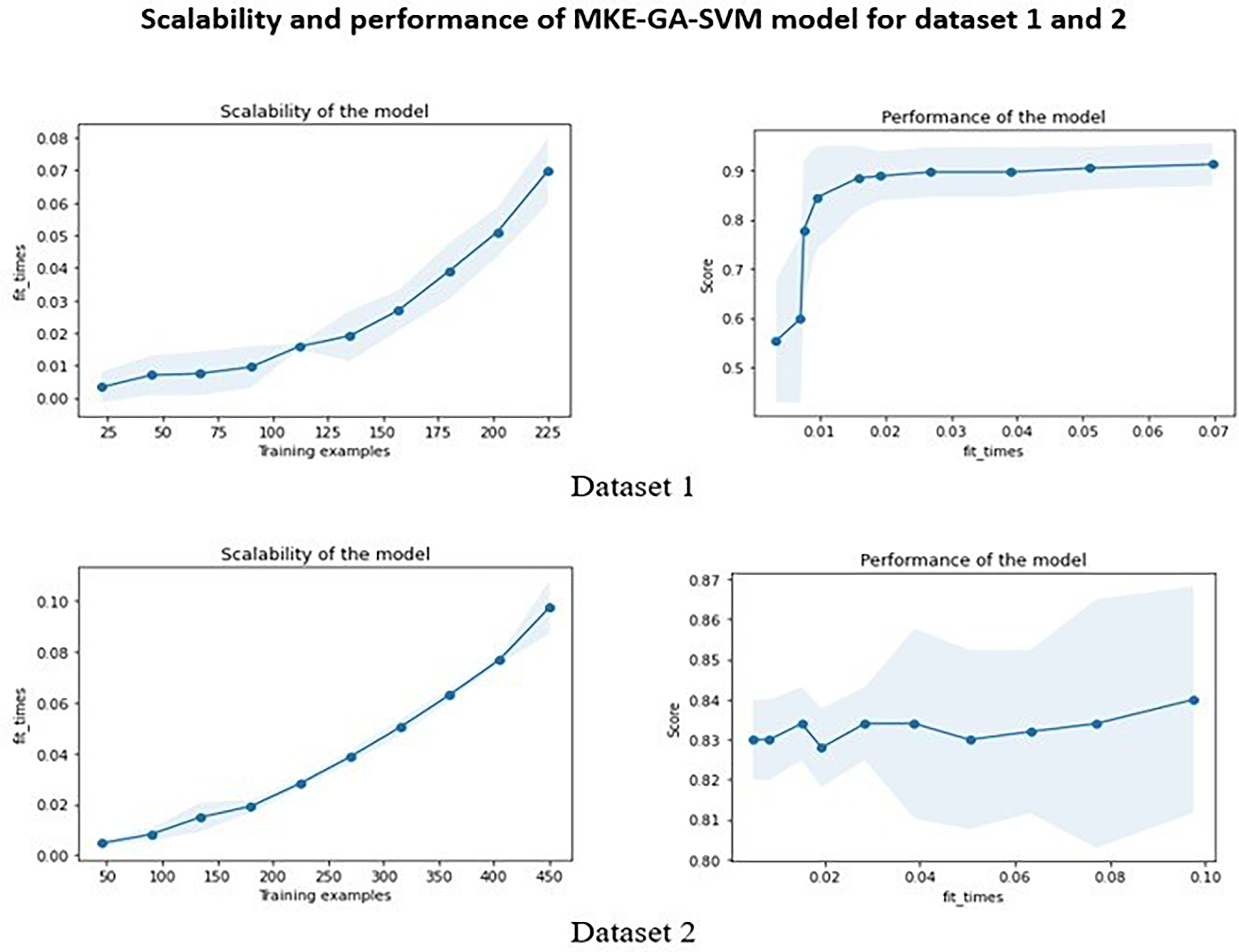
Scalability and performance of MKE-GA-SVM integrated model on dataset 1 and 2. The scalability of the model denotes the time required by the model to fit the estimator with the training dataset. The blue shaded region in the scalability graph indicates the region of fit_times mean +&− fit_times standard deviation. The performance of the model represents the test score with respect to fit_times. The blue shaded region indicates the region of test scores mean +&− test scores standard deviation.

Figure 6.

Scalability and performance of MKE-GA-SVM integrated model on dataset 3. The scalability of the model denotes the time required by the model to fit the estimator with the training dataset. The blue shaded region in the scalability graph indicates the region of fit_times mean +&− fit_times standard deviation. The performance of the model represents the test score with respect to fit_times. The blue shaded region indicates the region of test scores mean +&− test scores standard deviation.

Comparison with other standard models

The results of the newly created integrated model MKE-GA-SVM were compared to those of existing models that incorporate feature selection and hyperparameter tuning. These models include GA-SVM, Grid search-SVM, and the SVM-recursive feature elimination (RFE) model. The previous section has covered some of the fundamental information regarding these models. Table 2 displays the classification accuracy outcomes for the existing models and the MKE-GA-SVM integrated model on three datasets. The classification accuracies of the MKE-GA-SVM model on datasets 1, 2, and 3 were 91.4, 86.6, and 75.5, respectively, outperforming the outcomes of all other standard models in a convincing manner. Table 3 displays a comparison of the outcomes derived from assessing the respective models across three datasets, employing established evaluation metrics such as MSE, Log loss, AUC, and F1-score.

Table 2.

Classification accuracy MKE-GA-SVM and other compared models on three datasets.

	Classification Accuracy
Models	Dataset 1	Dataset 2	Dataset 3
MKE-GA-SVM	91.4	86.6	75.5
GA-SVM	84.2	83.3	68.6
Grid-SVM	90.3	82.3	74.5
SVM-RFE	90.4	84	71.4

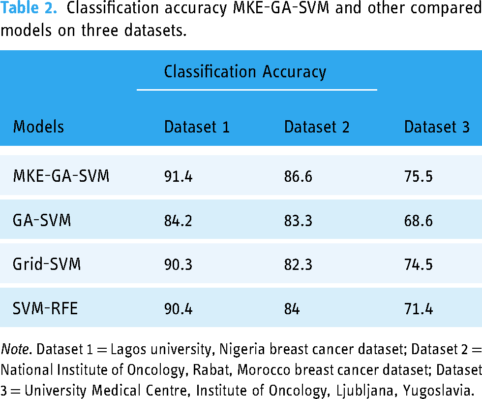
Note. Dataset 1 = Lagos university, Nigeria breast cancer dataset; Dataset 2 = National Institute of Oncology, Rabat, Morocco breast cancer dataset; Dataset 3 = University Medical Centre, Institute of Oncology, Ljubljana, Yugoslavia.

Table 3.

Several evaluation metrics comparative analyses of all models on dataset 1, 2 and 3.

	Dataset 1				Dataset 2				Dataset 3
Models	Mean square error (MSE)	Log loss	AUC score	F1-score	Mean square error (MSE)	Log loss	AUC score	F1-score	Mean square error (MSE)	Log loss	AUC score	F1-score
MKE-GA-SVM	0.06	0.85	0.94	0.93	0.13	0.38	0.73	0.80	0.31	0.69	0.44	0.55
GA-SVM	0.42	1.11	0.94	0.84	0.1	0.31	0.84	0.87	0.31	0.67	0.43	0.56
Grid-SVM	0.06	0.19	0.96	0.93	0.12	0.29	0.91	0.87	0.26	0.57	0.74	0.67
SVM-RFE	0.05	0.83	0.96	0.95	0.13	0.39	0.74	0.87	0.26	0.62	0.70	0.70

Note. Dataset 1 = Lagos university, Nigeria breast cancer dataset; Dataset 2 = National Institute of Oncology, Rabat, Morocco breast cancer dataset; Dataset 3 = University Medical Centre, Institute of Oncology, Ljubljana, Yugoslavia.

The MKE-GA-SVM model showcases substantial classification potential across all datasets, highlighted by its superior AUC and F1 scores, coupled with lower MSE and Log loss values.

The assessment of results for all models involved the application of the 10-fold cross-validation method to ensure robustness across three multi-centre datasets. Various kernel functions like radial basis, sigmoid, linear, and polynomial, and an array of evenly spaced range of C and gamma values in the logarithmic scale have been presented as options in this study and implemented in Python with the MKE algorithm to achieve the optimal SVM hyperparameter combination. As a result, the most suitable kernel function and optimize C, gamma values can be automatically evolved into an SVM hyperparameter combinations. Following the application of the MKE approach to datasets 1, 2, and 3, Table 4 presents the optimized values for SVM hyperparameters such kernel, C, and gamma. In dataset 1, a higher C parameter value shows that the MKE technique aims to minimize the misclassified samples at the expense of significant penalty value, whereas a smaller gamma value indicates significant similarity radius, enabling the inclusion of extra points to a specific class. The higher classification accuracy of dataset 1, which is 91.4%, lends more credence to this. Smaller C values for datasets 2 and 3 indicate that there is a significant margin for the SVM decision limit to accept greater misclassification. Consequently, datasets 2 and 3 have lower classification accuracy of 86.6% and 75.5% respectively. Therefore, the recently created bio-inspired integrated metaheuristic model may be used as a surrogate diagnostic tool to help the medical professionals offer patients with enhanced treatment outcomes.

Table 4.

Optimized hyperparameters values like kernel, C, and gamma of SVM generated by MKE technique on datasets 1, 2, and 3.

MKE-GA-SVM Model	Kernel	C	Gamma
Dataset 1	rbf	177.82	0.000177
Dataset 2	Rbf	3.83	0.21
Dataset 3	rbf	0.90	0.31

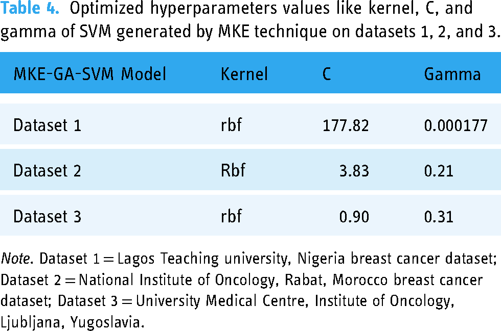
Note. Dataset 1 = Lagos Teaching university, Nigeria breast cancer dataset; Dataset 2 = National Institute of Oncology, Rabat, Morocco breast cancer dataset; Dataset 3 = University Medical Centre, Institute of Oncology, Ljubljana, Yugoslavia.

Statistical analysis

The correlation between categorical clinical and pathological attributes was determined using a heatmap in order to comprehend the relevance of clinicopathological parameters associated to breast cancer classification. Heatmaps, which are represented by colors of varied intensities, are produced to show the degree to which the clinicopathological factors are dependent on one another. Blue and red highlights were applied to the clinicopathological components in the heatmap based on the positive and negative correlations between them. Stronger shades of color are associated with larger correlation magnitudes. Dark blue shading along the diagonal of the heatmap denotes a correlation between the same variable and itself. The seaborn library in Python is used to create heatmaps. Figures 7, 8, and 9 illustrate the correlation heatmaps for datasets 1, 2, and 3, respectively. Age is positively correlated with menopausal status, nutritional status, hypertension, and comorbidity, according to the heatmap generated from dataset 1. Furthermore, correlation also exists between the histological type, disease stage, and metastasis. Age, menopause, the number of full-time pregnancies, hormone therapy, lymph nodes, tumor size with surgical type, and tumor advancement are factors in dataset 2 that have a positive correlation. Strong positive association lies between age and menopause, invading nodes and node-caps on dataset 3. Additionally, there prevails strength of association between tumor-size with invading nodes, node-caps and degenerative malignant. Irradiation and class are also positively correlated with each other.

Figure 7.

The correlation heat map of dataset 1. The higher correlation value among the clinicopathological parameters was indicated with the stronger colour shades. The dark clue colour heatmap diagonal signifies the correlation of the same variable with itself.

Figure 8.

The correlation heat map of dataset 2. The higher correlation value among the clinicopathological parameters was indicated with the stronger colour shades. The dark clue colour heatmap diagonal signifies the correlation of the same variable with itself.

Figure 9.

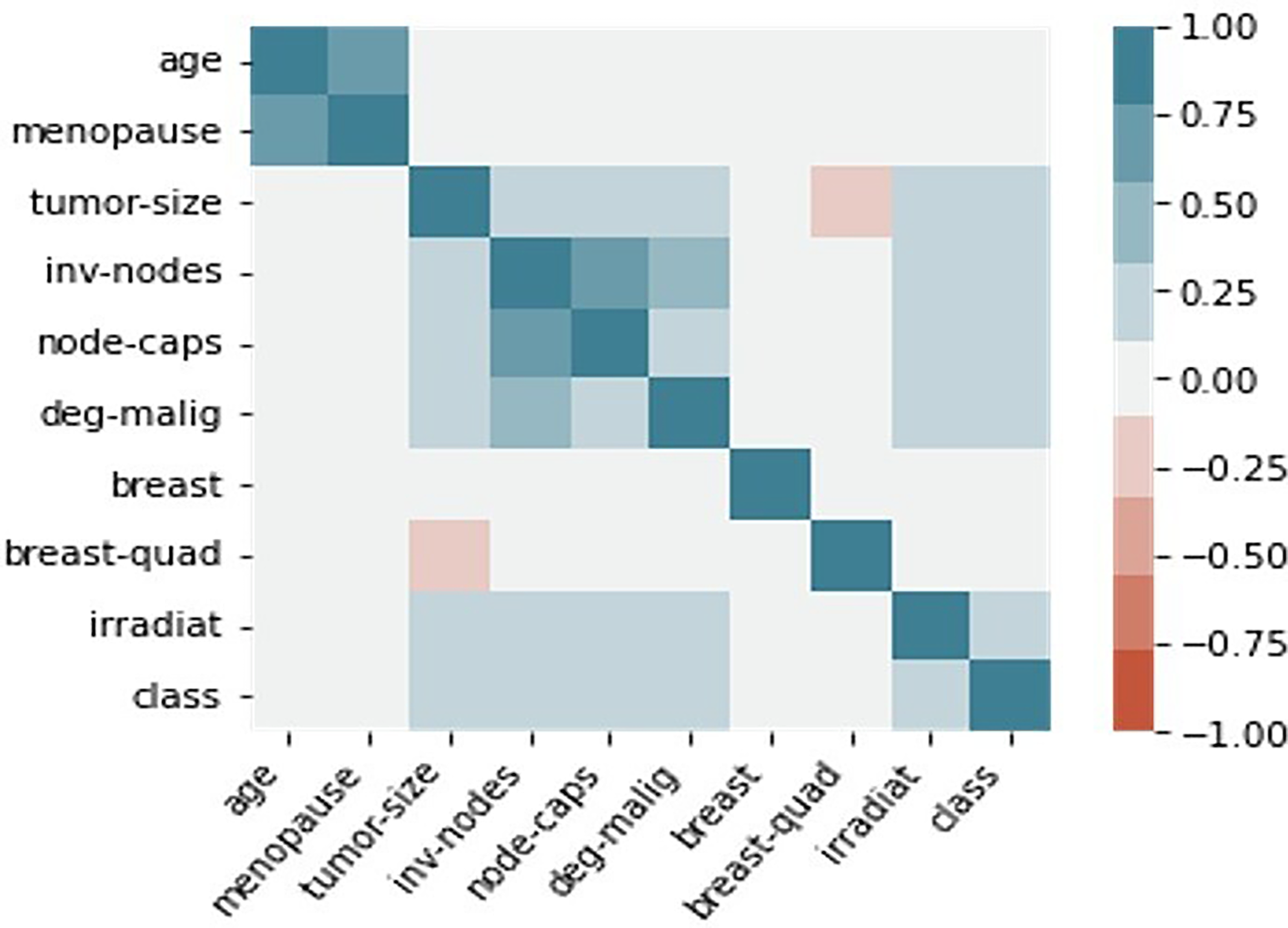
The correlation heat map of dataset 3. The higher correlation value among the clinicopathological parameters was indicated with the stronger colour shades. The dark blue colour heatmap diagonal signifies the correlation of the same variable with itself.

Pearson's chi-square test provides an alternative statistical method for examining the relationship between the clinicopathological characteristics of breast cancer patients. The chi-square statistic is calculated as the square of the difference between the actual and expected values for each categorical parameter, divided by the parameter's expected value.

$$\begin{array}{rl}{\chi }^2=& {\displaystyle \frac{{(O_{11}-E_{11})}^2}{E_{11}}+{\displaystyle \frac{{(O_{12}-E_{12})}^2}{E_{12}}+\dots }}\\ & +{\displaystyle \frac{{(O_{mn}-E_{mn})}^2}{E_{mn}}={\sum }_{i=1}^m{\sum }_{j=1}^n{\displaystyle \frac{{(O_{ij}-E_{ij})}^2}{E_{ij}}}}\end{array}$$

(6)

Here, τ stands for chi-square value, O_ij= observed value and E_ij= expected value of the categorical parameter. The aim of this test is to discern whether the difference between actual and expected values is attributable to chance or if there exists a meaningful relationship between the variables under investigation. The update of chi-square statistics takes into account the degree of freedom, which varies with the count of feature labels and class labels. The chi-square test was performed with Python version 3.11.2. The chi-square score, chi-square p-value, F-score, F-score p-value, and mutual information between the clinicopathological parameters are among the values that are produced as output. In dataset 1, clinicopathological characteristics, including patient height, BMI, family history of breast cancer, comorbidities, allergies, and hormone receptor status, were found to be statistically significant (p < .05) in distinguishing between TNBC cases and non-TNBC cases. Within dataset 2, hormone therapy and progression (metastasis/relapse) emerged as statistically significant clinicopathological variables (p < .05). In dataset 3, the clinicopathological variables that were statistically significant (p < .05) included tumor-size, invading nodes, node caps, degenerative malignant, and irradiation. These findings show that hormone therapy, metastasis/relapse, and hormone receptor status are among the risk variables associated with breast cancer's lethal effects. For more details, the original studies^38,40,42 presented a comprehensive statistical assessment of clinicopathological factors among TNBC and non-TNBC subgroups.

Discussion

Evaluation metrics, such as the area under the ROC curve (AUROC), MSE, logarithmic loss, PR curve, F1-score, and learning curves, were employed to assess and quantify the performance of the MKE-GA-SVM integrated model. Better classification accuracy was noted when comparing the outcomes with the feature selection and hyperparameter setting models of GA-SVM, Grid search-SVM, and SVM-RFE model. The major risk factors favouring the severity of breast cancer were also shown by the statistical analysis. This vindicated the overall potency of integrated model in segregating the patient groups with TNBC /non-TNBC and also its pivotal role in identifying the risk factors that influence the occurrence of recurrence/non-recurrence events. Few studies that combine MKE with other hybrid evolutionary strategies have been reported in the literature. A combination of canonical MKE technique and multi-trial vector strategy known as MMKE was suggested by Nadimi-Shahraki et al. ⁴⁸ to address a range of real-world optimization issues with diverse uncertainty. Li Zuoyong et al. ⁴⁹ employed an immune evolutionary algorithm to iteratively optimize the Monkey-king point, resulting in the Monkey-king immune evolutionary algorithm. This algorithm showcased improved searching capability and enhanced stability. In addition to these, several variants of the monkey king evolutionary algorithm have been developed and adopted in a variety of domains, including target-based wireless sensor networks (WSN), ⁵⁰ energy broadcast in WSN, ⁵¹ and vehicle navigation in a WSN environment. ⁵² However, the present study introduced a novel integrated model where the MKE method has been employed to identify the optimal settings of SVM hyperparameters, and GA was used to choose the pertinent clinical and pathological attributes involved in classification before being applied to the SVM classifier for prediction. While many studies^53,54 employ radial basis kernel functions as a baseline for SVM hyperparameter tuning, our present work in MKE explores a variety of alternative kernel functions. This approach is aimed at determining the best kernel function without being restricted to a specific choice. Our study likely represents the first reported instance of utilizing the MKE-GA-SVM integrated model for the automatic development of SVM hyperparameters in the categorization of patient groups: TNBC/non-TNBC based on clinicopathological criteria. But it is needless to mention that several models encompassing GA-SVM hybridization^55–59 are available in the literature for the diagnosis, classification, and prediction of breast cancer. The benefit of utilizing a hybrid model is that it unifies the complementing parameters of all the included models, which lessens the weaknesses that the separate classifiers experience. ⁶⁰ The study of medical datasets requires the use of ML techniques due to their extreme heterogeneity and complexity. In the literature, integrated ML models have started to appear as a remedy for this kind of complexity. In order to investigate breast cancer using an integrated ML approach (HMLA), Taghizadeh et al. ⁶¹ employed classifiers, a feature extraction strategy, and feature selection techniques in addition to comprehensive search for the best HMLAs. The medical sciences often use immunohistochemical staining, imaging, and radiomics to categorize breast cancer subtypes.^62–65 However, the application of ML integrated models, which have improved classification accuracy, provides a framework for effectively identifying tumours that are TNBC and those that are not, and it can be accepted as an addition to or replacement for medical procedures.

As per GLOBOCAN 2020, ⁶⁶ Africa has recorded 186,598 new instances of breast cancer, 85,787 instances with high mortality, and 429,220 cases per 100,000 of 5-year prevalence (across all age groups) rate. In addition, breast cancer ranks higher in Africa than cervix uteri cancer in terms of prevalence. The estimated incidence of breast cancer in females was 531,086 cases, or 74.3 cases per 100,000 women, but the number of deaths was 19.4 cases per 100,000, indicating a high breast cancer load in Africa. Researchers predict ⁶⁷ that by 2040, there would be 1.4 million cancer-related fatalities and 2.1 million new cases of cancer in Africa. The researchers observed that environmental risk factors and behavioural, in addition to food and lifestyle modifications, might be a cause of the increase. The researchers also emphasize that these increases will probably exceed the capacity of health care provider levels, postpone cancer screenings, and restrict patient treatment options unless measures are taken to raise awareness, enhance preventive, and minimize risk factors. This forces us to categorize breast cancer patients of African nations into TNBC versus non-TNBC subtypes. Destructive breast cancer TNBC, is typified by an aggressive tumour, a high occurrence in younger premenopausal women, an elevated risk of recurrence within the initial 3 years, and a diminished survival rate following metastasis. Due to their chemosensitivity, surgery combined with chemotherapy is frequently regarded as the accessible treatment methods, even though the FDA has not approved any particular targeted medications. In this study, statistical analysis reveals the relationship among the various clinicopathological traits and their degree of association. Chi-square statistic discloses the statistically significant clinicopathological traits that plays a pivotal role in identification of breast cancer patients into subtypes: TNBC and non/TNBC. These findings showcased the deadly impact of breast cancer and identified multiple risk factors, aiding clinicians in developing suitable treatment plans for both TNBC and non-TNBC categories of patients.

Artificial intelligence (AI), especially ML and deep learning, has found extensive applications in clinical cancer research in recent years. As a result, the accuracy of cancer prediction has significantly increased. Complex medical datasets may be analysed using ML approaches to find patterns and relationships, and they can also be used to accurately predict how a particular cancer subtype will progress in the future. Moreover, the prognosis of breast cancer patients can also be predicted using ML, which can be used as a resource for surgical selection technique, clinical patient evaluation, and adjuvant medication development. When medical data need to be evaluated more thoroughly and quickly, ML algorithms may be able to lessen the likelihood of human errors brought on by professionals who are drained or inexperienced. ML techniques have been used for breast cancer outcome prediction using tumour tissue imaging, ⁶⁸ ultrasonography imaging for TNBC patient diagnosis, ⁶⁹ and breast cancer survival prediction. ⁷⁰ Further, ML can produce positive outcomes with respect to the clinical care of patients.^71,72 The application of ML to the molecular classification of tumours has drawn more interest recently. Understanding the many molecular kinds of breast cancer can assist medical professionals in determining the optimal course of treatment for each patient, saving the health care system money and preventing undesirable side effects. ⁷³ However, before implementing any ML technique in clinical settings, privacy concerns pertaining to digital electronic health record (her) data must be effectively managed. Over the years, microarray-based method for BC categorization has been known as the gold standard. ⁷⁴ However, this method's primary drawback is that it fails to consistently classify samples into particular molecular subtypes.^75–77 Another significant issue is that individual's gene expression can change over time, which could lead to inaccurate classification results. The most popular screening technique for early-stage breast cancer is mammography.^78,79 The two prevailing constraints in adolescent women with thick breasts are low specificity and deteriorating sensitivity. Additionally, mammography's use of radiation is harmful for patient health and dramatically increases their risk of developing breast cancer. ⁸⁰ Ultrasonography has grown in popularity as a substitute for mammography in clinical use.^81–83 In contrast, uneven textural characteristics of low-quality ultrasound images frequently lead to inconsistent performance on new test instances. Moreover, diagnostic performance outperforms conventional visual imaging evaluations. These motivate us to come up with an ML model with integrated features for identifying breast cancer based on clinicopathological characteristics of patients in oncology or tertiary care facilities. Therefore, computer-aided diagnosis (CAD) systems have significant research value in aiding physicians to enhance the accuracy of breast tumour diagnosis.

Several literature reviews^84–88 have employed clinicopathological features and IHC staining for classifying patients into TNBC and non-TNBC groups. Notably, these studies have opted for statistical analysis using SPSS or other established software, rather than leveraging machine learning techniques for the automated diagnosis and treatment of breast cancer. The current study, however, presented a novel integrated model in which the evolutionary method of the monkey king was utilized to determine the ideal settings of the SVM hyperparameters. The single evolution approach and control parameter used by MKE have an impact on convergence and the ratio of exploration to exploitation. Given that evolution techniques greatly influence algorithm performance, combining several strategies can greatly improve algorithmic capabilities. To prevent MKE from prematurely convergent in local optima, optimization technique known as GA has been applied to enhance randomized searching capability and better stability. Prior to integrating GA with the SVM classifier for prediction, the relevant clinical and pathological factors that influence the classification process were selected. Such type of study with an MKE-GA-SVM integrated model was the first to be reported in the literature. In addition to precisely identifying breast cancer subtypes, our current research employs an integrated MKE-GA-SVM model to play a crucial role in pinpointing severe variants of TNBC. This identification is instrumental in determining targeted and improved treatment regimens for such cases. The validation of the current work with multicentre datasets from different geographic locations is particularly significant as it may be seen as a gap in earlier research findings. Finally, the integrated MKE-GA-SVM model has produced a data-driven diagnostic system that can help doctors to diagnose patients and plan appropriate courses of therapy.

Our ML integrated model underwent testing and evaluation, being benchmarked against the performance of three well-known hybrid approaches that involve both feature selection and hyperparameter tuning in the realm of ML. It's worth noting, however, that there are numerous other ML strategies that were not explored or taken into account in the scope of this study. This study did not investigate all types of breast cancer; there are various subtypes beyond TNBC. One potential limitation of this study could be the reduced dataset size derived from hospital-collected datasets with clinicopathological traits. To get around this problem, each dataset was subjected to a 10-fold cross-validation procedure, which produced 10 distinct models and allowed for prediction using all of the available data. The class imbalance issue that arises from the imbalanced design of TNBC and occurrence of recurrence events in datasets 2 and 3 can be resolved by using the SMOTE technique, which adds synthetic data to the k-nearest neighbors of the minority samples. Furthermore, the consequences on the diverse demographics of the patient populations were not considered. This highlights the potential limitation in the study.

Conclusion

The MKE-GA-SVM predictive model provides an alternative method for precise classification of breast cancer into TNBC and non-TNBC variants. Additionally, it can be utilized to detect recurrence events, helping the healthcare practitioners to deliver the most effective treatment and diagnostic results for patients. The findings indicated that the suggested MKE-GA-SVM classification model outperformed other existing models in terms of accuracy in predicting clinicopathological feature selection. Combining numerous breast cancer prognosis models predicting risk factors might improve disease detection and the formulation of critical treatment regimens. Predictive models are crucial for personalized medicine because they can easily identify high-risk people based on established clinical and pathological risks. More predictive methods should be investigated for improved prediction and accuracy in order to develop tailored treatment for the awful variety of breast cancer-TNBC.