Sage Journals: Discover world-class research

Abstract

Objective

Brain tumor grade is an important aspect of brain tumor diagnosis and helps to plan for treatment. Traditional methods of diagnosis, including biopsy and manual examination of medical images, are either invasive or may result in inaccurate diagnoses. This study proposes a brain tumor grade classification technique using a modern convolutional neural network (CNN) architecture called ConvNext that inputs magnetic resonance imaging (MRI) data.

Methods

Deep learning-based techniques are replacing invasive procedures for consistent, accurate, and non-invasive diagnosis of brain tumors. A well-known challenge of using deep learning architectures in medical imaging is data scarcity. Modern-day architectures have huge trainable parameters and require massive datasets to achieve the desired accuracy and avoid overfitting. Therefore, transfer learning is popular among researchers using medical imaging data. Recently, transformer-based architectures have surpassed CNNs for image data. However, recently proposed CNNs have achieved superior accuracy by introducing some tweaks inspired by vision transformers. This study proposed a technique to extract features from the ConvNext architecture and feed these features to a fully connected neural network for final classification.

Results

The proposed study achieved state-of-the-art performance on the BraTS 2019 dataset using pre-trained ConvNext. The best accuracy of 99.5% was achieved when three MRI sequences were input as three channels of the pre-trained CNN.

Conclusion

The study demonstrated the efficacy of the representations learned by a modern CNN architecture, which has a higher inductive bias for the image data than vision transformers for brain tumor grade classification.

Keywords

ConvNext convolutional neural networks transfer learning brain tumor grade

Introduction

A tumor is a tissue collection that grows abnormally and may become life-threatening. They become even more dangerous when they appear inside the brain, constrained by a limited space inside the skull.¹ The statistics show that brain tumor is found among patients belonging to almost all demographic groups.^2,3 Therefore, researchers from diverse domains strive to develop methods to diagnose and cure cancer. Like many other diseases, early diagnosis is crucial for diagnosing brain tumors.³

The treatment of a brain tumor strongly depends upon its type, which is determined by the type of brain cells from which it originated. For example, meningioma is a type of brain tumor that originates from a type of cells called meninges.⁴ Similarly, the tumorous mass originating from the pituitary gland is called a pituitary tumor. The most prevalent type of brain tumor is the one that originates from within the glial cells and is called Glioma.³ This research proposes a method for the diagnosis of Glioma.

An important aspect of brain tumor diagnosis is the grade of a tumor. It indicates the aggressiveness of the tumor or the rate at which it spreads itself. This rate of spread is strongly correlated to the expected days a patient will survive.³ Therefore, the grade of a brain tumor is crucial to plan for the patient's treatment.⁵ The World Health Organization divides tumors into four grades, starting from Grade 1 to Grade 4. Grade 1 tumors are the least aggressive, while Grade 4 tumors spread themselves fastest to nearby tissues. A further sub-division in this regard is low-grade Glioma (LGG) or high-grade Glioma (HGG), where the first two grades fall into the category of LGG, and Grades 3 and 4 are called HGG.³ The study proposes a classification technique to classify Glioma patients into LGG versus HGG.

A well-known problem in training machine/deep learning models in medical imaging is the need for more labeled data.⁶ Models pre-trained on generic datasets like ImageNet allow fine-tuning the models on target tasks with medical imaging data.⁷ Although several studies have used unlabeled medical data recently for self-supervised pre-training to achieve superior results, these methods are computationally expensive.⁸ Compute-intensive deep learning techniques contribute significantly to global carbon emissions, and this situation will likely exacerbate if the researchers do not prioritize compute efficiency.⁹

For many years, techniques based on the convolutional neural network (CNN) architecture have dominated the world of computer vision tasks and achieved state-of-the-art results.¹⁰ Several architectural innovations have been proposed, from skip connections in ResNets¹¹ to depth-wise convolutional layers in different Inception versions and Xception.¹² Neural architecture search techniques have allowed CNNs to perform better with optimal model sizes.¹³

However, recently, transformer-based architectures originally developed for language tasks have gained widespread acceptability for vision tasks and have achieved superior performance. Architectures like the Swin transformers have achieved better results and are scalable to higher image resolutions.¹⁴ Because of the superior results for many computer vision tasks, researchers have also used them for medical imaging tasks. However, transformer-based systems are significantly more computationally expensive than CNNs.

Although the Swin transformer has a higher inductive bias than the vanilla vision transformer (ViT), it is still less than the CNNs. This makes this ViT-based architecture more data-hungry and computationally expensive. This study aims to address this high computational and data requirements challenge by utilizing ConvNext,¹⁵ which has outperformed the Swin transformer on ImageNet while being computationally efficient. This study proposes a deep learning-based technique that works well with limited labeled data while using limited computational power available in the free tier of Google Colab using the pre-trained ConvNext. The features were extracted from ConvNext without fine-tuning the target data for brain tumor grade classification. The results achieved show the efficacy of the proposed approach.

A significant number of studies have utilized pre-trained architectures for medical imaging tasks. To our knowledge, studies have yet to use the pre-trained ConvNext architecture for this purpose. This study addresses this gap by utilizing the modern CNN architecture for brain tumor grade classification. The study assesses ConvNext's transfer performance of for the target task involving medical images.

More specifically, the following is the contribution of this study:

This study has shown that the representations learned by the modern CNN architecture of ConvNext achieved state-of-the-art performance for the target task of brain tumor grade classification.

Literature review

Traditionally, conventional machine learning methods have been used to classify medical images. However, classical techniques are still being proposed for medical imaging classification tasks because of the data-hungry nature of modern architectures. Following are the studies that used classical machine algorithms for medical imaging tasks.

The study¹⁶ proposed a pipeline to diagnose the brain tumor grade by first segmenting the tumorous region of the brain using a 3D architecture based on convolutional layers. Different features based on texture and shape were extracted from this region. Recursive feature elimination was used on a support vector machine (SVM) to select the most discriminating features. Finally, the extreme gradient boosting (XGBoost) classification algorithm was used to produce an accuracy of 91.27%. Although the study utilized features from only the relevant region, the handcrafted features could not fully capture the nuances in the data to achieve high accuracy.

The study¹⁷ used handcrafted features and an XGBoost classifier after feature selection to grade Gliomas. The first step was preprocessing, including wavelet transform and Laplacian of Gaussian. The next step was manual segmentation of the tumorous region. The feature extraction was performed only from the tumorous region instead of the whole image. Finally, the grade was classified after performing feature selection to achieve an accuracy of 83%. The study used the Shapley value to assess the contribution of different features towards the final classification. However, the study relied on manual segmentation, a laborious and expensive process.

The study¹⁸ used handcrafted feature extraction to extract the magnetic resonance imaging (MRI) images’ intensity, shape, and texture-based features. To eliminate redundant features, the correlation among different features was used, and only the discriminant features were kept. Finally, the random forest classifier was used for the final classification into LGG versus HGG. The study achieved an accuracy of 91.3% using BraTS 2015. The limitation of the proposed method is that it was validated on BraTS 2015 when newer and comparatively BraTS versions were available.

The study¹⁹ proposed a technique to classify Grade II versus Grade II Glioma. The dataset consisted of 36 patients and two sequences, contrast-enhanced T1-weighted (T1C) and fluid-attenuated inversion recovery (FLAIR). Different types of textural features were extracted from only the tumorous parts of the MRI scans. The redundant features were removed by calculating the correlation among the features, and only the discriminating features were retained. A random forest classifier was used to classify brain tumor grades. The best accuracy of 78.1% was achieved. Although the study compared the results of the proposed approach with the expert radiologist's diagnosis, the study used a tiny dataset.

The problem with classical machine learning methods is that they use handcrafted features that require human expertise to extract suitable features. With the ever-increasing sizes of medical imaging datasets and the emergence of unsupervised techniques that leverage unlabeled data and generative models, deep learning methods are now dominant among researchers. With the growing popularity of deep learning-based methods in the latter half of the previous decade, many tasks used pre-trained CNNs for medical image classification. Most of the techniques use pre-trained models as they cover up the limited size of the target datasets and produce superior results compared to the methods that train the models from scratch. The following studies have used deep learning-based techniques for tasks involving medical images.

To mitigate the impact of issues arising during the capturing of MRI scans, the study²⁰ performed preprocessing, including correcting the bias field. After that, the Gaussian filter is passed through the image to smooth it. The preprocessing is performed on a stack of four slices corresponding to the four MRI sequences, then passed to the long short-term memory (LSTM) model. The fully connected layer at the end classifies images into HGG versus LGG. The study achieved a best accuracy of 98% on BraTS 2018. The study introduced a novelty using a sequence model to process different MRI sequences.

The study²¹ utilized the pre-trained InceptionV3 CNN to extract deep features from MRI data. Before the feature extraction, the study performed contrast enhancement in the preprocessing phase. The proposed approach also extracted handcrafted features by utilizing a variant of the local binary pattern method. The deep and handcrafted features were concatenated and inputted to the next pipeline step, feature selection using particle swarm optimization. The study achieved the best accuracy of 96.9% on BraTS 2017. The study merged the deep and handcrafted features. However, Xception architecture had a better ImageNet accuracy by adopting the depthwise separable convolutions.

The study²² utilized the ImageNet pre-trained ResNet-152 for brain tumor grade classification. A softmax classifier replaced the classifier layer of the original architecture. The study used a deep architecture for the BraTS 2019 dataset and achieved an accuracy of 98.85%.

The study²³ proposed a novel CNN architecture modulated by Gabor filter so that the proposed CNN could extract the relevant imaging features from the MRI data. To enhance the results’ reliability, the study utilized the leave-one-patient approach. The results were compared with pre-trained CNNs like AlexNet, VGG-19, InceptionV1, and ResNet34. The proposed architecture outperformed all the pre-trained CNNs. Although the study proposed an innovation to the classical CNN architecture, its reliability could be enhanced by comparing it with the results obtained using modern CNN architectures.

The study²⁴ proposed and compared different brain tumor grade classification techniques using pre-trained CNNs and a novel CNN architecture. The features extracted from the pre-trained CNNs were fed to SVM for final classification. The datasets used to validate the proposed architecture were BraTS versions from 2017 to 2019. In addition to the development dataset, the study validated the approach on an external cohort to demonstrate the generalizability of the proposed method. The proposed novel architecture achieved the best accuracy across the development and external datasets. Although the novel architecture achieved good accuracy, it was worth using the modern pre-trained architectures and comparing the results with the state-of-the-art.

The study²⁵ used pre-trained EfficientNet architectures to classify brain tumor types. The classifier of EfficientNet architectures was discarded, and according to the task, a new classifier network was attached to the convolution base. The MRI data was preprocessed to reduce noise and discarding of the irrelevant image portions. The modified architectures were fine-tuned on the MRI data after data augmentation. The study utilized a modern CNN architecture, and the best result was achieved using EfficientNetB2 because of the dataset size.

The study¹⁰ proposed a novel CNN architecture to classify the abnormalities in a fetal brain using ultrasound images. The proposed architecture comprises bottleneck residual blocks, rectified linear unit non-linearity, batch normalization, and a max pooling layer for feature extraction. To select the distinguishing features, an optimization algorithm based on the modified MothFlame method was introduced to improve the classification accuracy and computational efficiency. The hyperparameters were optimized using the Bayesian method. The proposed approach achieved the best accuracy of 78.5%, significantly better than the state-of-the-art techniques. Although the study achieved superior accuracy using the proposed novel architecture, proposed hyperparameter selection, and feature selection method, the proposed approach may further be validated if it is applied to similar target tasks using the ultrasound modality.

The study²⁶ proposed three novel CNN architectures for diagnosing brain tumors into three types of classification: normal versus abnormal, type classification in Glioma, pituitary, and meningioma, and grade classification into Grades I–IV. The datasets used were Kaggle brain tumor type classification for normal versus Abnormal, Figshare CE-MRI for the type classification, and REMBRANDT for grade classification. The study performed preprocessing by noise removal and image quality enhancement using a median filter. Classical data augmentation techniques like image scaling and rotating the image by an angle were used to increase the dataset size. The complexities of the architecture depended upon the dataset size and the task complexity. Optimal hyperparameters were determined using the grid search. The study achieved the best accuracies of 99.4%, 97.78%, and 98.91% for the classification of normal versus Abnormal, brain tumor type, and brain tumor grade, respectively. The study proposed novel architectures, but better evaluation could be done by selecting a larger dataset, such as BraTS.

The study⁴ proposed an approach that used a modified ResNet50 architecture and autoencoder to extract features from MRI images. The features extracted from both architectures were fused. After performing the feature selection, a classifier network was used to classify the input data into the four MRI sequences (T1-weighted (T1), T1C, T2-weighted (T2), and FLAIR). The study achieved an accuracy of 99.8% on BraTS 2020 and 99.9% on BraTS 2021 and significantly outperformed the state-of-the-art methods. The study did not use modern CNN architectures that have significantly outperformed ResNet50 on ImageNet classification.

The study¹ utilized the pre-trained InceptionV3 architecture to extract the deep features and feed these features to the SVM classifier to classify MRI images as normal and abnormal. The images were normalized and resized before being put into the pre-trained InceptionV3. The study achieved an accuracy of 98.31% for normal versus abnormal classification. The authors used InceptionV3, but modern CNN architectures like EfficientNet and ConvNext have achieved superior performance and computational efficiency.

The study⁶ proposed a method to classify brain tumor type, fine-tuning the pre-trained CNNs EfficientNetB0 and InceptionResNetV2. An autoencoder-based data augmentation method was used to handle the imbalance in the dataset. Instead of manually searching for the optimal hyperparameters, the study used a Bayesian method to find suitable ones for fine-tuning the models. Finally, distinguishing features were selected using an algorithm called Marine Predator. After feature selection, a variety of classifiers were used for the classification. The best accuracy of 99.8% was achieved by feeding the discriminant features to the cubic SVM classifier, which outperformed the state-of-the-art methods. The study performed a thorough evaluation of the proposed pipeline by using a variety of classifiers and comparing the results with the state-of-the-art.

The transformer architecture was initially proposed for natural language data, but its variant vision transformer produced excellent results for the image classification tasks.²⁷ It was a radical shift from the sliding window-styled CNNs and used patches instead. The limitation of the vision transformer was its attention mechanism, which needed each patch to attend to every other patch. This design results in an exponential increase in the computational requirement with the increase in the resolution of input image data. Swin transformers presented a hybrid approach with patches and sliding windows. Swin transformer remained a dominant architecture for image data for a while.¹⁴ ResNext was an effort to revitalize CNN architecture by taking inspiration from the design choices of the Swin transformer, like the number of blocks in different stages, stem cell design, and depth-wise convolutions. The resulting architecture (ConvNext) outperformed the Swin transformer with fewer floating-point operations.¹⁵

This study uses a pre-trained CNN with a modern architecture (ConvNext Base) to extract features and then use these features for the target task of brain tumor grade classification. Figure 1 depicts the design choices and training strategies that helped ConvNext architecture achieve state-of-the-art performance.

Figure 1.

The design choices and training methodology of ConvNext are inspired by transformer-based architectures.¹⁵

Research methodology

This cross-sectional study uses a pre-existing, publicly available dataset to classify brain tumor grade using the proposed CNN-based technique. It was conducted in the Machine Perception & Visual Intelligence Research Group at the COMSATS University Islamabad, Lahore Campus, Pakistan, in the Spring of 2024. The publicly available dataset used in the study, BraTS 2019, was released in 2019. The block diagram of the proposed method is shown in Figure 2.

Figure 2.

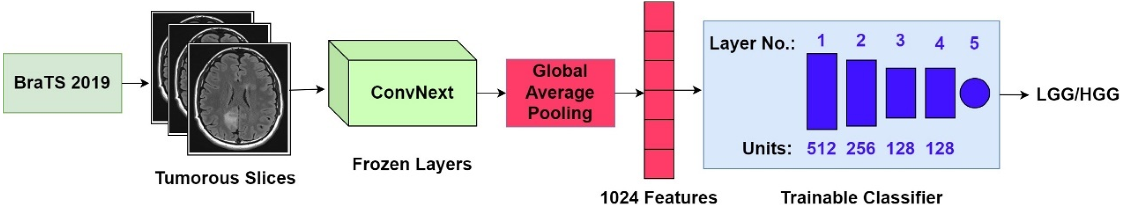
Block diagram of the proposed method.

In the first step of the pipeline, the tumorous slices were flagged. After that, the features were extracted only from the tumorous slices so the classifier gets the slices with either LGG or HGG tumor. For feature extraction, the study has used the regular version of the ConvNext called ConvNext Base by freezing all its layers. The pre-trained ConvNext's top model was discarded and replaced by a global average pooling layer that extracted one feature per feature map, thus resulting in a total of 1024 features. Finally, the features were provided to a fully connected neural network for classifying the data into LGG versus HGG. The sub-sections “Dataset,” “Deep features extraction,” and “Classification” present a detailed explanation of the dataset and methodology used by the study.

Dataset

The BraTS 2019 dataset was used in the study, and to the best of our knowledge, this is the first study that used this dataset for brain tumor grading using the features extracted from ConvNext.^28,29,30 BraTS is a popular publicly available dataset, and its different versions serve as a benchmark to compare techniques. As part of the BraTS 2020 dataset, a mapping of the datasets BraTS 2017, 2018, 2019, and 2020 was provided.^28,29,30,31 Of the 259 HGG patients, 210 are common in the 3 datasets, and the BraTS 2019 dataset contains an additional 49 patients. For LGG patients, 75 patients are the same in the 3 datasets, and BraTS 2019 has only 1 additional patient. The BraTS 2012 and 2013 cases are already included in these versions (2017 or later), while the BraTS 2014–2016 cases are discarded as they are not annotated by expert radiologists.³² BraTS 2020 contains an additional 34 HGG cases (compared to BraTS 2019), which makes the dataset further unbalanced. Based on this analysis, this study has used BraTS 2019.

The dataset consists of 76 LGG and 259 HGG cases, where each case has four sequences (T1, T2, T1 T1C, and FLAIR) and one ground-truth value, the manual tumor segmentation performed by expert radiologists. Each MRI scan for a sequence contains 155 slices, each with a dimension of 240 × 240. The acquisition protocol for T1 is 2D sagittal or axial, where each slice is 1–6 mm thick; for T1C, it is 3D and mostly with 1 mm thickness; for T2, it is 2D in axial orientation, and slices are 2–6 mm thick and finally for FLAIR it is 2D in all the orientations where slices are 2–6 mm thick. During manual segmentation (performed by the dataset providers), different parts of the tumor (edema, necrotic region, enhancing, and non-enhancing core) were delineated using different sequences or combinations. For each case, the delineations performed by various radiologists were fused to reach one consolidated segmentation.²⁸

The dataset was already preprocessed, and the proposed method did not perform further preprocessing. The preprocessing performed by the dataset providers was image registration and skull stripping. Registration was performed using rigid transformation, with the T1C sequence as the reference because of its highest spatial resolution. Skull stripping was then performed to remove the skull signal.

Features extraction and classification

Feature extraction in the proposed method was performed using the weights in the convolution base of ConvNext (Base version), which were pre-trained on the ImageNet dataset. Therefore, only the convolution base of ConvNext architecture was used, and its top model (optional fully connected layers and logistic regression) was discarded. Global average pooling was used, which resulted in 1024 features for each magnetic resonance slice. Instead of using all the slices, only the slices with the tumorous pixels were used. These tumorous slices were extracted using the ground truth segmentation provided by the dataset. The tumorous slices were fed to the pre-trained ConvNext without performing any further preprocessing step. To match the input dimensions of the pre-trained ConvNext, each slice was repeated three times to fill the three channels of the input layer.

The features extracted using the frozen layers in the convolution base of ConvNext and global average pooling were then fed to a fully connected neural network containing 754,945 trainable parameters. Table 1 shows the classifier network layers, the units in each layer, and the activation functions used.

Table 1.

The architecture of the classifier network.

Layer Number	Layer Type	Number of Units	Activation
1	Dense	512	ReLU
2	Dense	256	ReLU
3	Dense	256	ReLU
4	Dense	128	ReLU
5	Dense	1	Sigmoid

ReLU: rectified linear unit.

Two types of experiments were performed where in the first category of experiments, the convergence behavior was assessed by training the model for 500 epochs without using the validation set. Checkpoints were saved after each epoch and after training the test set accuracy was evaluated for each checkpoint, which helped in the visualization of the trajectory of the model to convergence for each setting. The best checkpoints for different input settings are given in Tables 4 and 7 and provide useful insight.

For the second category of experiments, a validation set was also used with early stopping regularization and a patience value of 20. After the training ended, the test set was evaluated on the best model (that produced the best accuracy on the validation set). The results obtained from the second category of experiments were compared with the state-of-the-art techniques for brain tumor grade classification. The rest of the hyperparameters were the same.

This study is a continuation of an earlier study³³ conducted to find the optimal pre-training strategy. Two models were used in the study³³: a simple and a complex model. The exact number of layers and units per layer and other hyperparameters were tuned empirically. This study retained the same hyperparameters and used the complex model (shown in Table 1). Table 2 shows the hyperparameter setting for the classification.

Table 2.

Hyperparameter settings for the classification.

Epochs	Batch Size	Learning Rate	Optimizer	Loss	Checkpoint Frequency
500	64	0.00005	Adam	Binary cross entropy	After every epoch

Statistical analysis

The accuracy measures the percentage of correctly classified examples in the test set. In addition to the overall accuracy, this study uses the measures of sensitivity (True Positive Rate) and specificity (True Negative Rate) to compute the class-specific accuracies to fairly represent the results in the presence of imbalanced classes. Moreover, the measure of AUC was used to assess the proposed approach's performance in a decision boundary-agnostic manner, offering a robust summary of the model's ability to distinguish between classes. The scikit-learn package in Python was used to calculate these metrics. The results for each sequence combination were compared using a horizontal bar graph. A bar was drawn for each metric, and the bars for the metrics of each sequence combination were grouped for better visualization of the performance difference among the individual and combined sequences. The Matplotlib library in Python was used to visualize the results.

Experimental settings

To increase the number of examples for training, 2D slices were used instead of 3D volumes, and only the slices marked as tumorous by radiologists were used. As a result, 4926 LGG and 17,224 HGG slices were obtained. For observing the training progress and convergence behavior, this data was divided into training and test sets using an 80–20 class balanced split, thus leaving 17,720 samples for training and 4430 for testing purposes where the size of each slice (sample) was 240 × 240. For the second category of experiments, 10% of the training set was allocated to the validation set. That means 15,948 slices were used to train the model, and 1772 were reserved for the validation set. Table 3 shows the images/slices of the train, test, and validation sets.

Table 3.

Slices/images in the train, test, and validation sets.

Class	Train Set	Test Set	Validation Set	Total Tumorous Slices
HGG	12,401	3445	1378	17,224
LGG	3547	985	394	4926
Total	15,948	4430	1772	22,150

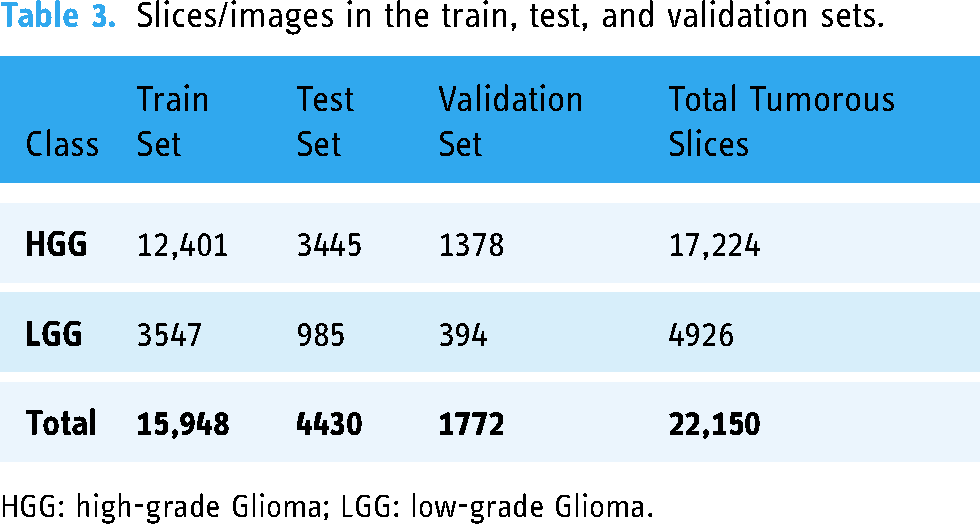
HGG: high-grade Glioma; LGG: low-grade Glioma.

Experiments were performed on each possible combination of the sequences. Since the feature extraction was performed using the pre-trained ConvNext, input was limited by having precisely three channels. Therefore, only a combination of any three sequences could be used. Each sequence occupied one channel of the input tensor.

Results

Experiments were performed for each possible combination of any three sequences. The evaluation measures used are accuracy, sensitivity, specificity, and area under the curve (AUC). LGG has been treated as the negative class, while HGG has been treated as the positive class. Therefore, sensitivity is the percentage of HGG examples that are correctly classified, while specificity is the percentage of correctly classified LGG examples.

To study the training progression and convergence behavior, the model was trained for 500 epochs in each experiment, and checkpoints were saved after every epoch. The best results (accuracy, sensitivity, specificity, and AUC) of each experiment (a combination of sequences) are shown in Table 4. The best accuracy in the table has been highlighted in bold.

In the second category of experiments (grade classification using train, test, and validation sets), the training epochs were again set to 500. However, the training stopped much earlier for each experiment because of the early stopping with a patience of 20. The test set results (accuracy, sensitivity, specificity, and AUC) of each experiment (a combination of sequences) are shown in Table 5. The best accuracy in the table has been highlighted in bold.

Table 4.

The best accuracy (and other measures) was achieved for each combination using 500 epochs.

Sequence(s)	Results
Sequence(s)	Best Accuracy (%)	Sensitivity (%)	Specificity (%)	AUC (%)	Epoch Number
T1, T1C, T2	99.59	99.82	98.58	82.58	282
T1, T1C, T2, FLAIR	99.61	99.8	98.88	99.98	175
T1, T2, FLAIR	99.37	99.59	98.48	99.88	132
T1C, T2, FLAIR	99.37	99.68	98.17	99.94	159

AUC: area under the curve; T1: T1-weighted; T1C: contrast-enhanced T1-weighted; T2: T2-weighted; FLAIR: fluid-attenuated inversion recovery.

Table 5.

The accuracy (and other measures) achieved for each combination using early stopping.

Sequence(s)	Results
Sequence(s)	Accuracy (%)	Sensitivity (%)	Specificity (%)	AUC (%)	Epochs Before Convergence
T1, T1C, T2	99.16	99.21	98.98	99.98	44
T1, T1C, FLAIR	99.5	99.62	99.09	99.97	46
T1, T2, FLAIR	99.11	99.56	97.56	99.98	42
T1C, T2, FLAIR	99.03	99.3	98.07	99.91	52

AUC: area under the curve; T1: T1-weighted; T1C: contrast-enhanced T1-weighted; T2: T2-weighted; FLAIR: fluid-attenuated inversion recovery.

The best accuracy (99.61% and 99.5%) was achieved for the combination of T1, T1C, and FLAIR sequences in both types of experiments. The lowest accuracy (99.37% and 99.03%) was achieved for the combination of T1, T1, T1C, and FLAIR, which both involved the FLAIR sequence. The top two best accuracies were achieved for the combinations involving T1 and T1C. Manual segmentation performed on the BraTS dataset's magnetic resonance images explains these results. Although the radiologists used all the sequences for labeling the data, T1 was used along with T1C to segment different tumor substructures.²⁸

Comparison with studies using BraTS 2017 or later

The study results (of experiments using a validation set) have been compared with those using BraTS 2017 and 2018 as these two datasets are closest to BraTS 2019, while the previous BraTS datasets are different. The study³⁴ only used a tiny subset of the data from BraTS 2013 and 2017 (only 60 images for training and 100 for testing). Therefore, it is not included in the comparison (although it reported an accuracy of 99%). A comparison of the proposed method with the studies using BraTS 2017 or later for brain tumor grading has been presented in Table 6.

Table 6.

Comparison of the proposed approach with existing techniques.

	Study	Dataset	Accuracy
Classical machine learning methods	³⁵	BraTS 2017	88.77
	³⁶	BraTS 2017	91.18
	³⁷	BraTS 2018	91.18
	³⁸	BraTS 2018	98.71
Deep learning methods	³⁹	BraTS 2017	89.47
	⁴⁰	BraTS 2019	98.85
	⁴¹	BraTS 2017	92.98
	²⁰	BraTS 2018	98
	⁴²	BraTS 2017	92.4
	⁴³	BraTS 2017	97.78
	²¹	BraTS 2017	96.9
	²¹	BraTS 2018	92.5
	⁴⁴	BraTS 2017	90.87
	⁴⁵	BraTS 2018	97.1
	⁴⁶	BraTS 2018	96.1
	⁴⁷	BraTS 2018	96.49
	²³	BraTS 2017	98.68
	⁴⁸	BraTS 2017	90.7
	⁴⁹	BraTS 2019	95.86
	²⁴	BraTS 2017	97.85
	²⁴	BraTS 2019	97.15
	Proposed method	BraTS 2019	99.5

Table 7.

The best accuracy (and other measures) was achieved for individual sequences using 500 epochs.

Sequence(s)	Results
Sequence(s)	Best Accuracy (%)	Sensitivity (%)	Specificity (%)	AUC (%)	Epoch Number
T1	99.12	99.59	97.36	99.67	74
T1C	98.85	99.48	96.34	99.83	60
T2	99.05	99.53	97.26	99.82	61
FLAIR	99	99.42	97.26	99.74	60

AUC: area under the curve; T1: T1-weighted; T1C: contrast-enhanced T1-weighted; T2: T2-weighted; FLAIR: fluid-attenuated inversion recovery.

Ablation study

Studies have used individual sequences and have copied the same slice three times to form a three-channel input. The purpose of the ablation study was to see the result when only one sequence was used. Each of the four sequences was used to gauge the best sequence.

Table 7 presents the results when using individual sequences to study the training progression and convergence behavior.

Table 8 presents the results when using individual sequences with early stopping based on the validation set metrics. In Tables 7 and 8, the best results are highlighted in bold.

Table 8.

The best accuracy (and other measures) was achieved for individual sequences using early stopping.

Sequence(s)	Results
Sequence(s)	Accuracy (%)	Sensitivity (%)	Specificity (%)	AUC (%)	Epochs Before Convergence
T1	98.55	99.27	96.04	99.75	46
T1C	97.88	98.87	94.42	99.67	33
T2	97.47	98.98	92.18	99.6	46
FLAIR	97.97	98.72	95.33	99.49	35

AUC: area under the curve; T1: T1-weighted; T1C: contrast-enhanced T1-weighted; T2: T2-weighted; FLAIR: fluid-attenuated inversion recovery.

It is evident from the results that a combination of sequences produces better classification accuracy than individual sequences. For individual sequences, the best accuracy was achieved for T1 (99.12% and 98.55%). Interestingly, the top two best results achieved for a combination of sequences involved the T1 sequence. The lowest accuracy for a combination of sequences is greater compared to the best accuracy of individual sequences. Also, all the combinations of sequences took more epochs to converge (reach the highest accuracy) compared to the individual sequences. MRI sequences contain complementary information, and radiologists use multiple sequences to segment brain tumors manually. The CNN architecture also achieved superior results when presented with comprehensive information compared to when identical sequences were used for each input channel.

The results of Tables 4 and 7 are visualized in Figure 3 for a better comparison of the results in the ablation study with the regular experiments.

Figure 3.

Visualization of the results achieved for experiments using 500 epochs.

Discussion

The results showed that the proposed method achieved superior accuracy and outperformed the state-of-the-art when inputting three different MRI sequences to the CNN. Many studies used BraTS datasets and compared the results obtained using individual sequences and their combinations for brain tumor grading. The study⁴² used convolutional autoencoders for brain tumor grading on the BraTS 2017 dataset by performing pre-training using synthetic images generated through the generative adversarial network and then fine-training on the actual images. Three sequences (T1C, T2, and FLAIR) were used individually and in combination. The best and average results were reported using the combination of these three sequences, while for individual sequences, the best accuracy was reported using T1C. The study¹⁸ performed brain tumor grading through radiomic features and a random forest classifier on the BraTS 2015 dataset. All the sequences (T1, T1C, T2, and FLAIR) and their possible combinations were used for classification, and the results were compared. The lowest accuracy was reported using individual sequence features (FLAIR), a combination of two sequences performed better than individual sequences, and a combination of three sequences performed better than a combination of two sequences. In comparison, the best accuracy was achieved when features from all four sequences were merged and fed to the classifier. T1C achieved the best accuracy for individual sequences, while for a combination of the two, the best accuracy was reported using T1C and T1. The best accuracy was reported for three sequences using the combination of T1, T1C, and T2. Finally, the study³⁷ used texture features and logistic regression to classify grades on the BraTS 2018 dataset. Different sequences (T1C and T2) combinations and tumor regions (necrotic and edema) were used for grade classification. The best result was reported using the combination of T1C and T2 when features from only the necrotic region were classified.

The study's results were compared to the recent studies that used classical machine learning and deep learning techniques. The studies^35,36,37,38 used classical machine learning algorithms for brain tumor grade classification. The study³⁶ used texture features and a logistic regression classifier,³⁵ and used shape-based, histogram-based, and texture features. At the same time, the best accuracy was achieved using a random forest classifier. The study³⁷ used texture features and, after performing feature selection, fed them to regular neural networks for grade classification.

The rest of the studies given in the comparison table (Table 6) used CNNs except for two studies, one of which used convolutional autoencoder,⁴² while the other used LSTM for grade classification.²⁰ The studies^39,41,43,47 proposed novel CNN architectures, while the study²¹ used deep features extracted from pre-trained InceptionV3 along with dominant rotated local binary pattern features for grade classification. The study²³ used novel CNN where the Gabor filter bank modulated convolutional layers to add rotation and scale invariance to the learned features. The study⁴⁸ increased the dataset size by using semi-supervised learning to estimate the labels of unlabeled data and generative adversarial network (GAN) to generate synthetic data. The study⁴⁰ used deep features and fed them to the softmax after selecting the optimal features.

Conclusion and future works

The success of the Swin transformer provided the research community with design choices that were used to design and train the ConvNext architecture and achieve state-of-the-art performance. The stronger inductive bias of the CNN architecture makes them more suitable for the image data. These characteristics make ConvNext a suitable architecture for medical imaging tasks with smaller dataset sizes. This study uses the pre-trained ConvNext architecture for the brain tumor grade classification. The study used linear probing after extracting the features of the BraTS 2019 dataset from the ConvNext architecture. The superior results in accuracy, sensitivity, specificity, and AUC on the target task of brain tumor grade classification demonstrated the efficacy of the representations learned from the pre-trained ConvNext architecture.

The study presented results using ConvNext representations for a target medical image task. However, more studies are needed for a comprehensive investigation involving many imaging modalities, organs, and anomalies. To ensure generalizability, the study needs to be conducted on datasets of different sizes, starting from small to medium to large ones. Also, the efficacy of different versions of the ConvNext architecture needs to be investigated.

Recently, domain-adapted pre-training has been used by many researchers to achieve better results compared to the generic dataset pre-trained models. The in-domain data pre-training after the generic dataset (e.g. ImageNet) pre-training was able to bridge the domain difference between the generic dataset and target dataset (e.g. MRI). It would be interesting to see the performance of ConvNext after domain-adaptive pre-training compared to the generic dataset pre-training. The lottery ticket method and its variants are another compute-efficient training technique that results in a model with much fewer parameters while achieving comparable accuracy. It is worthwhile to explore the target task performance of a pre-trained model using such methods. Finally, some studies have slightly modified the pre-trained models to accommodate the target data with more channels in the data (e.g. MRI). Since using all the sequences results in comprehensive information about a subject, exploring the computationally efficient methods suggested in this section while using all the sequences during the target classification is necessary.

Footnotes

Contributorship

YM was involved in conceptualization, methodology, software, validation, formal analysis, investigation, resources, data curation, writing—original draft, writing—review and editing, and visualization. UIB was involved in conceptualization, methodology, validation, formal analysis, resources, data curation, writing—review and editing, and supervision.

Data availability statement

The BraTS 2019 dataset^28,29,30 used in this study can be obtained by posting a request through the web page .

Declaration of conflicting interests

The authors declared no potential conflicts of interest with respect to the research, authorship, and/or publication of this article.

Ethical approval

This research uses the publicly available BraTS 2019 dataset. The providers have explicitly included a “Data Usage Agreement/Citations” on the dataset homepage that allows any non-commercial use of the dataset. Therefore, this research requires no approval from any ethics committee.

Funding

The authors received no financial support for the research, authorship, and/or publication of this article.

Guarantor

UIB. ORCID iD: 0000-0001-5755-1194

Informed consent

This research does not require informed consent from the patients as this research uses data that is publicly available.

ORCID iDs

Yasar Mehmood

Usama Ijaz Bajwa

References

Lamba

Rani

Khan

, et al. RE-InCep-BT-: Resource-efficient InCeptor model for brain tumor diagnostic healthcare applications in computer vision. Mobile Netw Appl 2024: 1–15.

National Brain Tumor Society. Brain tumor facts. https://braintumor.org/brain-tumors/about-brain-tumors/brain-tumor-facts/ (accessed 12 March 2024)

DeAngelis

. Brain tumors. N Engl J Med 2001; 344: 114–123.

Ullah

Khan

Almujally

, et al. Brainnet: A fusion assisted novel optimal framework of residual blocks and stacked autoencoders for multimodal brain tumor classification. Sci Rep 2024; 14: 5895.

Tandel

, et al. A review on a deep learning perspective in brain cancer classification. Cancers (Basel) 2019; 11: 111.

Ullah

Khan

Masood

, et al. Brain tumor classification from MRI scans: A framework of hybrid deep learning model with Bayesian optimization and quantum theory-based marine predator algorithm. Front Oncol 2024; 14: 1335740.

Raghu

Zhang

Kleinberg

, et al. Transfusion: Understanding transfer learning for medical imaging. Adv Neural Inf Process Syst 2019; 32.

Balestriero

, et al. A cookbook of self-supervised learning. arXiv preprint arXiv:2304.12210 2023.

Lannelongue

Grealey

Inouye

. Green algorithms: Quantifying the carbon footprint of computation. Adv Sci 2021; 8: 2100707.

10.

Rauf

, et al. Automated deep bottleneck residual 82-layered architecture with Bayesian optimization for the classification of brain and common maternal fetal ultrasound planes. Front Med (Lausanne) 2023; 10: 1330218.

11.

Zhang

Ren

, et al. Deep residual learning for image recognition. Proceedings of the IEEE conference on computer vision and pattern recognition 2016: 770–778.

12.

Chollet

. Xception: Deep learning with depth wise separable convolutions. IEEE conference on computer vision and pattern recognition (CVPR) 2017: 1251–1258.

13.

Zoph

Vasudevan

Shlens

, et al. Learning transferable architectures for scalable image recognition. Proceedings of the IEEE conference on computer vision and pattern recognition 2018: 8697–8710.

14.

Liu

, et al. Swin transformer: Hierarchical vision transformer using shifted windows. Proceedings of the IEEE/CVF international conference on computer vision 2021: 10012–10022.

15.

Liu

Mao

C-Y

, et al. A convnet for the 2020s. Proceedings of the IEEE/CVF conference on computer vision and pattern recognition 2022: 11976–11986.

16.

Chen

Liu

Peng

, et al. Computer-aided grading of gliomas combining automatic segmentation and radiomics. Int J Biomed Imaging 2018; 2018: 1–11.

17.

Xiao

, et al. Game theoretic interpretability for learning based preoperative gliomas grading. Future Gener Comput Syst 2020; 112: 1–10.

18.

Cui

, et al. Machine-learning-based classification of lower-grade gliomas and high-grade gliomas using radiomic features in multi-parametric MRI. arXiv preprint arXiv:1911.10145 2019.

19.

Zhao

S-S

, et al. Better efficacy in differentiating WHO grade II from III oligodendrogliomas with machine-learning than radiologist’s Reading from conventional T1 contrast-enhanced and fluid attenuated inversion recovery images. BMC Neurol 2020; 20: 1–10.

20.

Amin

Sharif

Raza

, et al. Brain tumor detection: A long short-term memory (LSTM)-based learning model. Neural Comput Appl 2020; 32: 15965–15973.

21.

Sharif

Khan

, et al. Active deep neural network features selection for segmentation and recognition of brain tumors using MRI images. Pattern Recognit Lett 2020; 129: 181–189.

22.

Athisayamani

Antonyswamy

Sarveshwaran

, et al. Feature extraction using a residual deep convolutional neural network (ResNet-152) and optimized feature dimension reduction for MRI brain tumor classification. Diagnostics 2023; 13: 668.

23.

Singh

Goel

Raghuvanshi

. Computer-aided diagnostic network for brain tumor classification employing modulated gabor filter banks. Vis Comput 2021; 37: 2157–2171.

24.

Hafeez

, et al. A CNN-Model to Classify Low-grade and High-grade Glioma from MRI Images. IEEE Access 2023; 11.

25.

Zulfiqar

Bajwa

Mehmood

. Multi-class classification of brain tumor types from MR images using EfficientNets. Biomed Signal Process Control 2023; 84: 104777.

26.

Gull

Akbar

Naqi

. A deep learning approach for multi-stage classification of brain tumor through magnetic resonance images. Int J Imaging Syst Technol 2023; 33: 1745–1766.

27.

Dosovitskiy

, et al. An image is worth 16 ( 16 words: Transformers for image recognition at scale. arXiv preprint arXiv:2010.11929 2020.

28.

Menze

, et al. The multimodal brain tumor image segmentation benchmark (BRATS). IEEE Trans Med Imaging 2014; 34: 1993–2024.

29.

Bakas

, et al. Advancing the cancer genome atlas glioma MRI collections with expert segmentation labels and radiomic features. Sci Data 2017; 4: 1–13.

30.

Bakas

, et al. Identifying the best machine learning algorithms for brain tumor segmentation, progression assessment, and overall survival prediction in the BRATS challenge. arXiv preprint arXiv:1811.02629 2018.

31.

Bakas

, et al. Segmentation labels and radiomic features for the pre-operative scans of the TCGA-GBM collection. The Cancer Imaging Archive 2017; 9. https://doi. org/10.7937K

32.

U. of P. Perelman School of Medicine. Multimodal brain tumor segmentation challenge 2017. https://www.med.upenn.edu/sbia/brats2017/data.html.

33.

Mehmood

Bajwa

Sun

. Resource-efficient domain adaptive pre-training for medical images. arXiv preprint arXiv:2204.13280 2022.

34.

Polly

Shil

Hossain

, et al. Detection and classification of HGG and LGG brain tumor using machine learning. In: 2018 International conference on information networking (ICOIN). Chiang Mai, Thailand: IEEE, 2018, pp.813–817.

35.

Cho

Lee

Kim

, et al. Classification of the glioma grading using radiomics analysis. PeerJ 2018; 6: e5982.

36.

Garcia

JGS

López

JMH

Barbosa

, et al. Texture analysis applied to brain MRI to classify low and high grade gliomas. in AIP conference proceedings 2019, p. 2090.

37.

Suárez-Garcia

Hernández-López

Moreno-Barbosa

, et al. A simple model for glioma grading based on texture analysis applied to conventional brain MRI. PLoS One 2020; 15: e0228972.

38.

Asthana

Hanmandlu

Vashisth

. Classification of brain tumor from magnetic resonance images using probabilistic features and possibilistic Hanman–Shannon transform classifier. Int J Imaging Syst Technol 2022; 32: 280–294.

39.

IY-H

, et al. 3D multi-scale convolutional networks for glioma grading using MR images. 2018 25th IEEE international conference on image processing (ICIP) 2018: 141–145.

40.

Athisayamani

Antonyswamy

Sarveshwaran

, et al. Feature extraction using a residual deep convolutional neural network (ResNet-152) and optimized feature dimension reduction for MRI brain tumor classification. Diagnostics 2023; 13: 668.

41.

Pereira

Meier

Alves

, et al. Automatic brain tumor grading from MRI data using convolutional neural networks and quality assessment. In: Understanding and interpreting machine learning in medical image computing applications: First international workshops, MLCN 2018, DLF 2018, and iMIMIC 2018, held in conjunction with MICCAI 2018, Granada, Spain, September 16–20, 2018, proceedings 1. Springer, 2018, pp.106–114.

42.

Ali

IY-H

Jakola

. Multi-stream convolutional autoencoder and 2D generative adversarial network for glioma classification. In: Computer analysis of images and patterns: 18th international conference, CAIP 2019, Salerno, Italy, September 3–5, 2019, proceedings, part I 18. Springer, 2019, pp.234–245.

43.

Amin

Sharif

Anjum

, et al. Convolutional neural network with batch normalization for glioma and stroke lesion detection using MRI. Cogn Syst Res 2020; 59: 304–311.

44.

Nadeem

, et al. Brain tumor analysis empowered with deep learning: a review, taxonomy, and future challenges. Brain Sci 2020; 10: 118.

45.

Zhuge

, et al. Automated glioma grading on conventional MRI images using deep convolutional neural networks. Med Phys 2020; 47: 3044–3053.

46.

Anilkumar

Kumar

. Multi tumor classification in MR brain images through deep feature extraction using CNN and supervised classifier. Int J Emerg Technol 2020; 11: 83–90.

47.

Mzoughi

, et al. Deep multi-scale 3D convolutional neural network (CNN) for MRI gliomas brain tumor classification. J Digit Imaging 2020; 33: 903–915.

48.

IY-H

Jakola

, et al. Deep semi-supervised learning for brain tumor classification. BMC Med Imaging 2020; 20: 1–11.

49.

Tripathi

Bag

. An attention-guided CNN framework for segmentation and grading of glioma using 3D MRI scans. IEEE/ACM Trans Comput Biol Bioinform 2022; 20: 1890–1904.

Brain tumor grade classification using the ConvNext architecture

Abstract

Objective

Methods

Results

Conclusion

Keywords

Introduction

Literature review

Research methodology

Dataset

Features extraction and classification

Statistical analysis

Experimental settings

Results

Comparison with studies using BraTS 2017 or later

Ablation study

Discussion

Conclusion and future works

Footnotes

Contributorship

Data availability statement

Declaration of conflicting interests

Ethical approval

Funding

Guarantor

Informed consent

ORCID iDs

References