Sage Journals: Discover world-class research

Abstract

Objectives

Diabetes is a metabolic disease and early detection is crucial to ensuring a healthy life for people with prediabetes. Community care plays an important role in public health, but the association between community follow-up of key life characteristics and diabetes risk remains unclear. Based on the method of optimal feature selection and risk scorecard, follow-up data of diabetes patients are modeled to assess diabetes risk.

Methods

We conducted a study on the diabetes risk assessment model and risk scorecard using follow-up data from diabetes patients in Haizhu District, Guangzhou, from 2016 to 2023. The raw data underwent preprocessing and imbalance handling. Subsequently, features relevant to diabetes were selected and optimized to determine the optimal subset of features associated with community follow-up and diabetes risk. We established the diabetes risk assessment model. Furthermore, for a comprehensible and interpretable risk expression, the Weight of Evidence transformation method was applied to features. The transformed features were discretized using the quantile binning method to design the risk scorecard, mapping the model's output to five risk levels.

Results

In constructing the diabetes risk assessment model, the Random Forest classifier achieved the highest accuracy. The risk scorecard obtained an accuracy of 85.16%, precision of 87.30%, recall of 80.26%, and an F1 score of 83.27% on the unbalanced research dataset. The performance loss compared to the diabetes risk assessment model was minimal, suggesting that the binning method used for constructing the diabetes risk scorecard is reasonable, with very low feature information loss.

Conclusion

The methods provided in this article demonstrate effectiveness and reliability in the assessment of diabetes risk. The assessment model and scorecard can be directly applied to community doctors for large-scale risk identification and early warning and can also be used for individual self-examination to reduce risk factor levels.

Keywords

Diabetes risk assessment type 2 diabetes community follow-up optimal feature selection scorecard

Introduction

Diabetes is a metabolic disease¹ that clinically presents as chronic hyperglycemia, abnormal blood lipids and proteins, and other symptoms that increase the risk of morbidity and mortality,² including kidney disease, vision loss, and heart disease.³ Diabetes has become a rapidly growing chronic health problem worldwide.^4,5 The major risk factors for diabetes are considered to be unhealthy diet, aging, family history, race, obesity, sedentary lifestyle, and previous history of gestational diabetes.^6,7 Previous studies have also reported that gender, body mass index (BMI), pregnancy, and metabolic status are associated with diabetes.^8,9 Early detection and symptomatic treatment are crucial to ensure the healthy life and well-being of individuals with prediabetes.^10–13

With the continuous advancement of technology, machine learning and deep learning techniques have become very useful in early prediction and disease analysis.^14–17 In recent years, many algorithms have been used to predict diabetes. Polat and Güneş¹² used Neuro fuzzy inference and 10-fold cross-validation on the Pima Indian dataset to obtain an Accuracy of 89.47%, and displayed Age, BMI, number of pregnancies, glucose tolerance test result, diastolic blood pressure, Features such as triceps skin fold thickness, 2-h serum insulin, and diabetes pedigree function are diabetes-associated parameters. Yu et al.¹³ used Support Vector Machine and 10-fold cross-validation on NHANES (National Health and Nutrition Examination Survey) USA to obtain 83.5% area under curve (AUC) and display family history, age, gender, race and ethnicity, weight, height, waist circumference, BMI, hypertension, physical activity, smoking, alcohol use, education, and household income are diabetes-related parameters. López et al.¹⁸ used Random forest (RF) and 10-fold cross-validation in Girona, Spain to obtain an AUC of 89%, and showed that Genetic data (Single nucleotide polymorphisms, SNP), age, BMI, and sex are related to diabetes parameter. Zou et al.¹⁹ used RF and 5-fold cross-validation in Chinese hospital to obtain 80.8% accuracy and displayed age, pulse rate, breath, left systolic pressure (SP), right SP, left diastolic pressure, right diastolic pressure, height, weight, physique index, fasting glucose, waistline, low-density lipoprotein (LDL), and high-density lipoprotein (HDL) are diabetes-related parameters. Dinh et al.²⁰ used XGBoost (an ENSEMBL model) and 10-fold cross-validation on NHANES (National Health and Nutrition Examination Survey, USA), obtained an AUC of 84.4%, and showed 24 most important variables out of 123: blood osmolality, sodium, blood urea nitrogen, triglyceride, LDL, age, waist, leg length, chloride, self-reported greatest weight, close relative had diabetes, total cholesterol, gamma–glutamyl transferase, ethnicity, systolic blood pressure, HDL, pulse, carbohydrate intake, general health condition, mean cell volume, aspartate aminotransferase, lymphocyte number, and white blood cell count are parameters associated with diabetes. Han et al.²¹ built three binary classification models to distinguish normal fasting plasma glucose (NFG) from mildly impaired fasting plasma glucose (IFG), NFG from type 2 diabetes (T2DM), and IFG from T2DM, using XGBoost as the basic classifier based on the Beijing Physical Examination Center dataset. NFG (fasting plasma glucose [FPG] < 6.1 mmol/L), IFG (6.1 mmol/L ≤ FPG < 7.0 mmol/L), T2DM (FPG > 7.0 mmol/L). The AUCs of these models on the test data set were 78.08%, 86.87%, and 70.67%, respectively. They used the Gini impurity index to evaluate the importance of features, sorted them according to the importance of features, combined with the incremental feature selection strategy to mine-related risk factors, showing that age, triglycerides ester, waist height ratio, and SP are important risk factors. Phongying and Hiriote²² proposed new diabetic classification models that incorporate hyperparameter tuning and the addition of some interaction terms into the models. For the four machine learning techniques, decision trees, RFs, support vector machines, and K-nearest neighbors (KNN), the models with interaction terms have better classification performance. Among the models with interaction terms, the RF classifier exhibits the best performance. To provide a more intuitive assessment of the risk of diabetes, in recent years, multivariable risk scores have been developed to predict the risk of diabetes in the general population. These risk scores are recommended in current chronic disease prevention guidelines and have been implemented in prevention programs in some countries. A study²³ developed a score based on routinely collected information to identify individuals at potential risk of undiagnosed diabetes. Another study²⁴ conducted a cross-sectional analysis using data from the Rancho Bernardo study (age 67 ± 11 years) to establish a predictive rule that could predict abnormal PCPG ≥140 mg/dl in nondiabetic participants. A study²⁵ developed and validated a simplified Indian Diabetes Risk Score (IDRS) for detecting undiagnosed diabetes in India. The IDRS was derived from the Chennai Urban Rural Epidemiology Study and was developed based on the results of multiple logistic regression (LR) analysis. Internal validation was conducted on the same data. In a study,²⁶ a random population sample of men and women aged 35–64 who had not received any antidiabetic medication treatment at baseline and were followed up for 10 years. A multinomial LR model was used to assign a score to each variable category. The diabetes risk score was composed of the sum of these individual scores.

Diabetic patients manage chronic diseases through community follow-up services. These studies have achieved good model performance, but the sample data used in the research are not directly from community follow-up, and cannot be effectively used for large-scale screening and early warning in the community. In order to overcome the shortcomings of the previous model, we directly extracted the daily diabetes follow-up data from the community service management information system and developed a risk assessment model and scorecard based on real large-scale data, which is conducive to the large-scale popularization of the model and facilitates community follow-up doctors to patients rapid identification screening.

Materials and methods

System design

We first preprocess the acquired community follow-up data (variable transformation, outlier processing, missing value processing), and then use oversampling for data balance to obtain a balanced data set, and select the optimal feature subset through three feature selection techniques. Then, use six algorithm models to train and verify the data set to obtain the optimal prediction algorithm model. Finally, create a diabetes risk scorecard. The whole research process is shown in Figure 1.

Figure 1.

Research flowchart.

Patients and data sets

We obtained community follow-up records of type 2 diabetes patients from 2016 to 2023 from the grassroots community service management system in Haizhu District, Guangzhou. There are a total of 16 initial parameters. According to actual needs and clinical experience, we deleted six features that are not related to the label. For example, BMI is a more reasonable indicator to evaluate a person's physical fitness, so we deleted the weight. The description of the 10 parameters is as follows:

BMI: Body Mass Index.

Age: Age.

Smoking: Smoking status, in units of cigarettes, 20 cigarettes per pack.

Staple_food: Staple food, measured in grams.

Exercise_frequency: Exercise frequency, which refers to the number of exercises per week.

Exercise_time: The duration of a workout, in minutes.

Drinking: drinking state, with Chinese Baijiu as the unit.

Systolic_BP: Systolic blood pressure.

Diastolic_BP: Diastolic blood pressure.

Diabetes: 0 means no diabetes, 1 means diabetes. In the dataset, there are 188,753 instances with label 0 and 63,423 instances with label 1.

In order to facilitate feature collection for clinical applications, we added three new features. In order to explore the relationship between limb blood pressure difference and diabetes, the index pressure difference of systolic blood pressure and diastolic blood pressure is added. The three new features are calculated as follows:

BMI_age = BMI * Age.

Exercise_total_time = Exercise_frequency * Exercise_time.

Diff_BP = Systolic_BP - Diastolic_BP.

In order to eliminate the noise in the initial data and obtain high-quality data, we have done a series of data preprocessing. First, the text feature code is converted into a discrete variable, and the abnormal range data are eliminated. Then, the samples with missing values are deleted, and the duplicate samples are deleted. The final processed data set has a total of 252,176 records, including 13 parameters, with 12 features.

Data balancing processing

Through the statistics of the processed data set according to the target value of diabetes classification, we found that 74.8% of the samples are labeled 0, and 25.2% of the samples are labeled 1. The data set is unbalanced. When traditional classification algorithms perform binary classification on a dataset, they usually assume that the number of samples in the class to be classified in the dataset is approximately equal. If traditional classification algorithms are used for binary classification of imbalanced data, the original classification boundary is easily affected by small class samples. If this method is used to train the sample data set, the decision boundary will be shifted and classification errors will occur. There are two ways to equalize the samples: undersampling and oversampling. The former achieves interclass sample balance by deleting some majority class samples, while the latter achieves interclass sample balance by generating minority class samples. Because undersampling may lose the effective information of the original sample set, resulting in inaccurate classification, most of the current related research uses oversampling.²⁷ We evaluated the skewness of the key features of the data set, converted them to normal distribution using nonlinear scaling, and then used three oversampling methods, namely synthetic minor oversampling technique (SMOTE), adaptive synthetic sampling (ADASYN), RandomOverSampler, and two undersampling methods, RandomUnderSampler and Near Miss, to balance the data set. And draw histograms of the dataset before and after equalization, as well as the scatter distribution after dimensionality reduction, and select a more suitable equalization algorithm based on the distribution of main features.

Skewness

Skewness is a measure of the direction and degree of skewness in the distribution of statistical data, which is a numerical characteristic of the degree of asymmetry in the distribution of statistical data. The characteristic number that characterizes the degree of asymmetry of the probability distribution density curve relative to the average value. Skewness is the third-order normalized moment of the sample.^28,29 The definition formula is as follows:

S k e w (X) = E [(\frac{X - μ}{σ})^{3}] = \frac{k_{3}}{σ^{3}} = \frac{k_{3}}{k_{2}^{3 / 2}}

(1)

where

k_{2}

and

k_{3}

represent the second-order and third-order central moment, respectively.

The skewness of normal distribution is 0, and the tail length on both sides is symmetrical. If bs represents skewness, bs < 0 means that the distribution has a negative deviation, also known as left skewness. At this point, there are fewer data on the left side of the mean than on the right side, which is intuitively manifested as the left tail being longer compared to the right tail, because a few variables have small values, causing the left tail of the curve to drag too long; If bs > 0, the distribution has a positive deviation, also known as a right skewness. At this point, there are fewer data on the right side of the mean than on the left, which is intuitively manifested as the tail on the right side being longer compared to the tail on the left, because a few variables have large values, causing the tail on the right side of the curve to drag too long; If bs approaches 0, it can be considered that the distribution is symmetric.

Synthetic minor oversampling technique

The SMOTE algorithm is a common algorithm for imbalanced data augmentation proposed by Chawla et al.³⁰ Its basic principle is to expand the data by random linear interpolation between a few samples and their neighbors to achieve a certain imbalance ratio. The imbalance ratio is the ratio of the number of few class samples to the number of many class samples in the sample set.

The specific steps of the SMOTE algorithm are: for any small class sample $x_{i}$ (i = 1, 2,…, n), calculate the distance between $x_{i}$ and other small class samples, and obtain the k nearest neighbors of sample $x_{i}$ . Then, m nearest neighbor samples are randomly selected from k nearest neighbors, recorded as $x_{i j}$ (j = 1, 2,…, m), and new few class samples are constructed by random linear interpolation between $x_{i}$ and $x_{i j}$ . The interpolation formula is:

x_{n e w} = x_{i} + r a n d (0, 1) (x_{i j} - x_{i})

(2)

Among them,

x_{n e w}

represents a small class of artificially constructed samples, and rand(0,1) is a random number that satisfies a uniform distribution on the interval (0,1).

Adaptive synthetic sampling

The ADASYN algorithm comes from small class sample points that are adaptively synthesized. This method synthesizes subcategory sample points based on their distribution status. The algorithm steps are as follows:³¹

Determine the number of samples to generate:

G = (m_{l} - m_{s}) \times β

(3)

$m_{l}$ represents the number of existing majority class samples; $m_{s}$ represents the number of existing minority samples; $β$ ∈[0, 1], when β = 1, the number of minority and majority class samples after synthesis is equal.

Calculate the proportion of majority class samples among the K nearest neighbors of each minority class sample:

r_{i} = Δ_{i} / K

(4)

$Δ_{i}$ is the number of majority class samples in K nearest neighbors of the i-th minority class sample, i = 1, 2,…, $m_{s}$ .

Standardized $r_{i}$ :

{\hat{r}}_{i} = r_{i} / \sum_{i = 1}^{m_{s}} r_{i}

(5)

Calculate the number of new samples to be generated for each minority sample:

g_{i} = {\hat{r}}_{i} \times G

(6)

G represents the total number of samples that need to be generated.

For each minority class sample $x_{i}$ , generate gi new samples according to the following equation:

s_{i} = x_{i} + (x_{z i} - x_{i}) \times λ

(7)

s_{i}

represents the generated sample;

x_{z i}

is a randomly selected minority class sample from the K nearest neighbors of

x_{i}

;

λ

is a random number,

λ

∈[0,1].

RandomOverSampler

Random oversampling is to increase the number of minority samples in the dataset by copying them, so as to achieve the goal of category balance. Assuming the number of minority class samples is $N_{-} m$ . The number of samples in most classes is $N_{-} M$ . If the multiple of oversampling is k (i.e., minority samples are copied k times), the number of samples after oversampling is:

N_{-} m^{'} = k \times N_{-} m

(8)

N_{-} M^{'} = N_{-} M

(9)

RandomUnderSampler

Random undersampling is achieved by deleting the majority of class samples to reduce their number in the dataset, thereby achieving class balance. Mathematically, assuming the number of samples in most classes is $N_{-} M$ . The number of minority samples is $N_{-} m$ . If the undersampling multiple is k (i.e., the proportion of deleting most class samples), the number of samples after undersampling is:

N_{-} m^{'} = N_{-} m

(10)

N_{-} M^{'} = k \times N_{-} M

(11)

Near Miss

Near Miss reduces the number of majority class samples by selecting minority class samples that are close to the majority class samples. There are several variants of the Near Miss algorithm: Near Miss-1, Near Mis-2, and Near Mis-3. We use Near Miss-1.

Near Miss-1 selects the K minority class samples closest to the majority class samples and retains them in the undersampled dataset. Mathematically, assuming the number of samples in most classes is $N_{-} M$ . The number of minority samples is $N_{-} m$ . If the number of neighbors is K, and the number of samples after undersampling is $N^{'}$ , then Near Miss-1 is expressed as follows:

N^{'} = K \times N_{-} M

(12)

Characteristic selection of diabetes

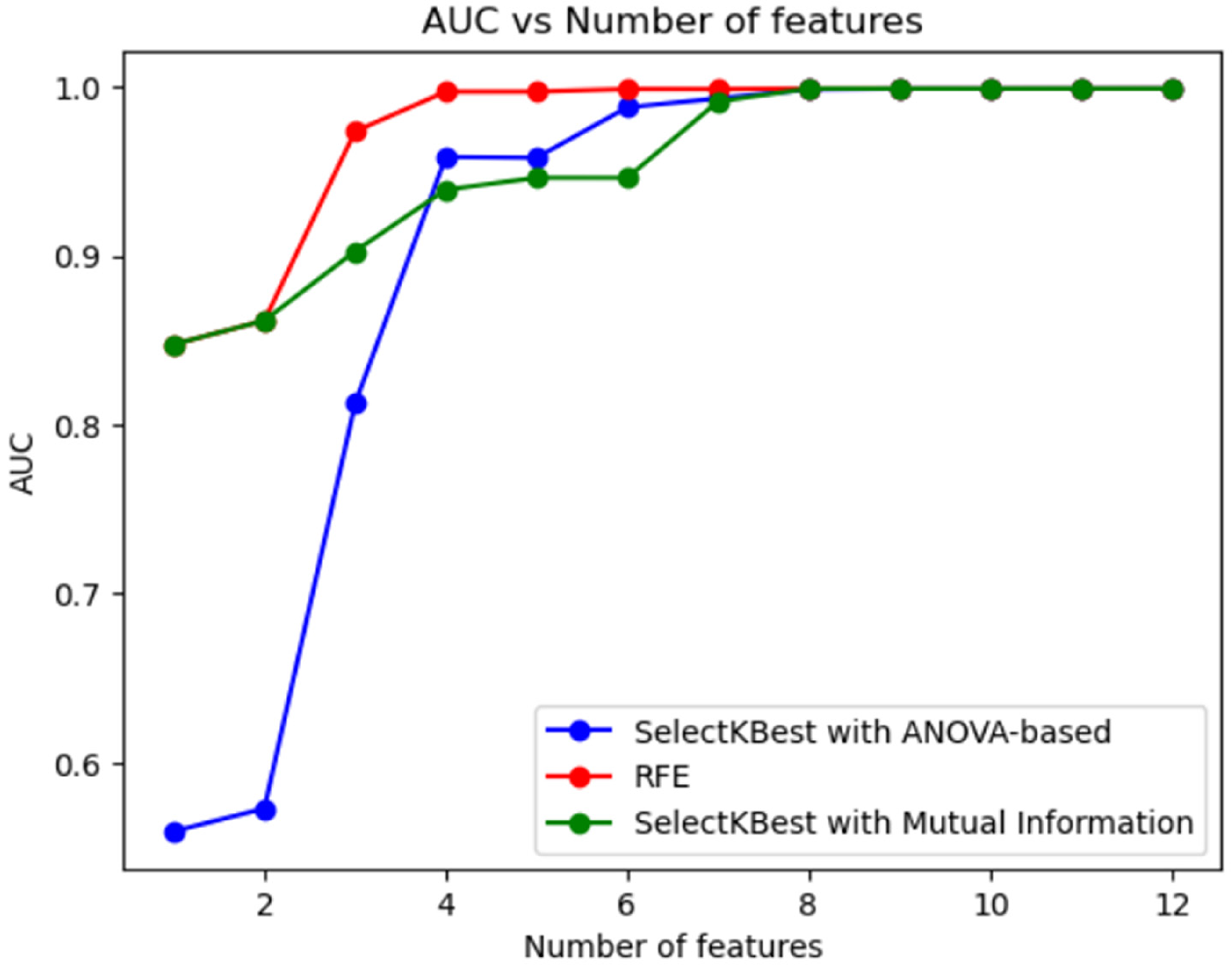
Feature selection aims to filter out features that may carry redundant information, and the goal is to find the optimal feature subset.³² Feature selection can eliminate irrelevant or redundant features, thereby achieving the purpose of reducing the number of features, improving model accuracy, and reducing running time. On the other hand, the truly relevant features are selected to simplify the model. We evaluated three feature selection methods, SelectKBest with ANOVA-based, Recursive Feature Elimination (RFE), and SelectKBest with Mutual Information, comparing the relationship between different numbers of features and the AUC score of a RF classifier.

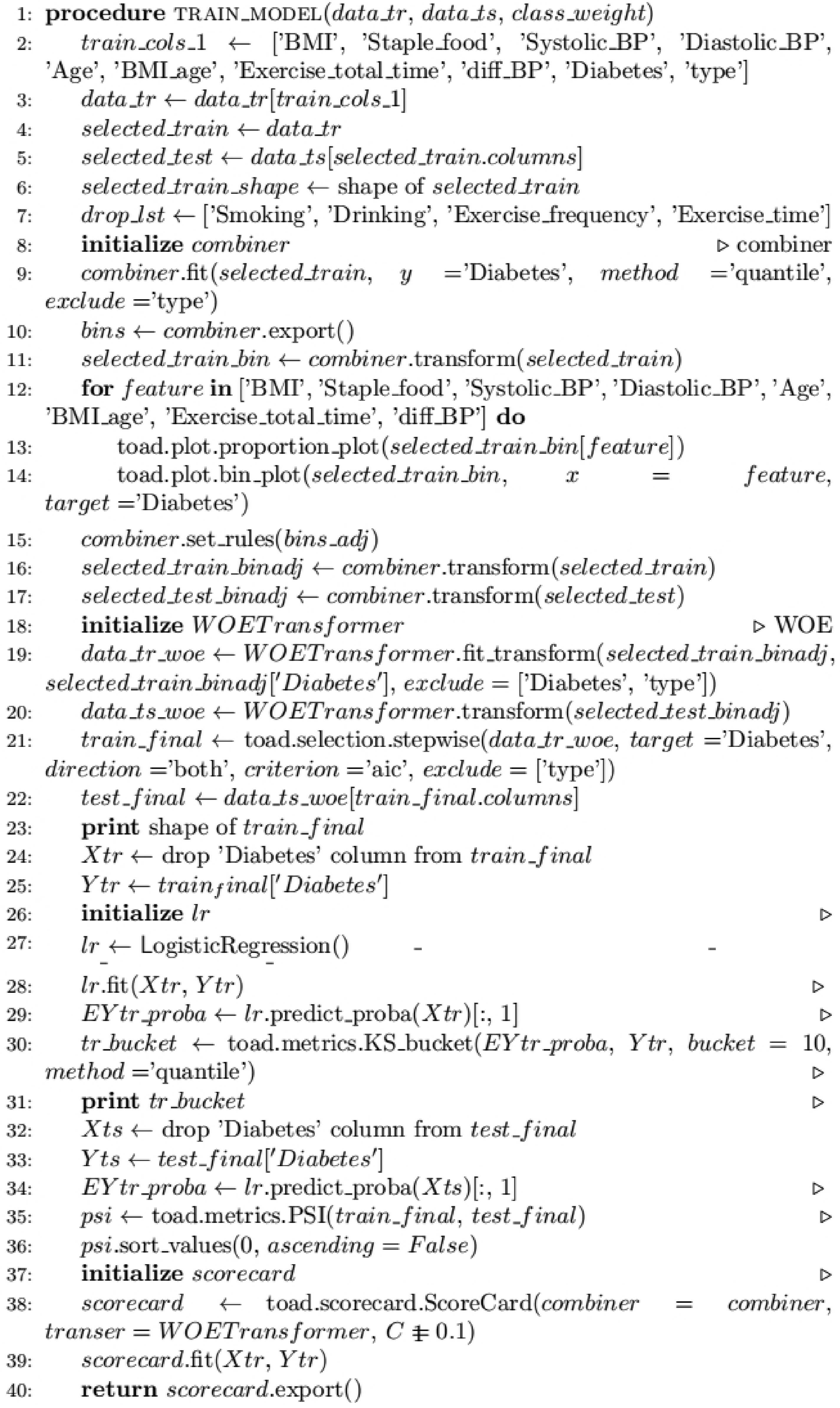
For each method, a range of values of k is traversed (selecting the number of features to select), the feature selection method is fitted on the training data, the training and test data are transformed using the selected features, the data are scaled using the StandardScaler, using the RandomForestClassifier with default hyperparameters on the scaled data, the ROC AUC score for the training data was calculated. See Appendix A for pseudocode.

Selectkbest with ANOVA-based

SelectKBest with ANOVA is an analysis of variance (ANOVA)-based feature selection method suitable for classification problems. It calculates the variance ratio (F-value) between each feature and the target variable, sorting the features based on these values. The top k features with the highest F-value are then selected.

When using SelectKBest, specify the desired number of features, denoted as k, and the chosen statistical test method, in this case, ANOVA. For the training data, SelectKBest calculates the F-value for each feature in relation to the target variable, ultimately selecting the top k features with the highest F-value. Applying this same subset of features to the test data ensures consistency in the feature space between the training and test datasets.

Recursive feature elimination

Recursive feature elimination is a model-based feature selection method that can be used for classification or regression problems. It selects features by recursively training the model and discarding the least important features.

When using RFE, you need to specify the number of features k to be selected and the model to use (RandomForestClassifier is selected here). Then, for the training data, RFE first trains a base model containing all features, then sorts the features according to their importance, removes the least important features, trains the model again, and repeats this process until k features are selected. Use the same subset of features on the test data to ensure that the training and test data have the same feature space.

SelectKBest with mutual information

SelectKBest with Mutual Information is a feature selection method based on mutual information, applicable to classification or regression problems. It calculates the mutual information between each feature and the target variable, sorting the features based on these values. The top k features with the highest mutual information values (IVs) are then selected.

When using SelectKBest, it is essential to specify the desired number of features, denoted as k, and the chosen statistical test method, in this case, Mutual Information. For the training data, SelectKBest calculates the mutual information for each feature in relation to the target variable, selecting the top k features with the highest mutual IVs. Employing this identical subset of features on the test data ensures consistency in the feature space between the training and test datasets.

Classification algorithm

After obtaining the optimal eight features, we used six models to evaluate the predictive performance of diabetes,^33–39 namely Random Forest (RF), Gradient Boosting Decision Tree (GBDT), eXtreme Gradient Boosting (XGB), K-Nearest Neighbors (KNN), Multilayer Perceptron (MLP), and Ensemble Learning (VC), in order to achieve the best good forecast. We evaluate model results using a confusion matrix. The performance of the model is evaluated using four evaluation indicators: accuracy (Acc), sensitivity (Sens), precision (Pre), and F1 score.^40–42

Random forest

Random forest is a VC algorithm based on decision trees. By randomly selecting samples and features, a classifier composed of multiple decision trees ${h (x, θ_{k})}$ is generated, where ${θ_{k}}$ are mutually independent and identically distributed random vector. Finally, the final class label of the input vector x is determined comprehensively by all decision tree votes.

In order to construct k trees, k random vectors $θ_{1}, θ_{2}, \dots θ_{k}$ need to be generated first, and these random vectors $θ_{i}$ are independent of each other and have the same distribution. The random vector $θ_{i}$ is used to construct the decision classification tree $h (x, θ_{i})$ , which is simplified as $h_{i} (x)$ . In the process of constructing the tree, according to the principle of minimum node impurity, a feature is randomly selected from the features for branch growth. In the risk prediction of diabetes, RF can predict the risk of disease according to the combination of multiple variables.

$I$ is an indicator function used to assess whether a condition holds true. In this context, the condition is $h_{i} (x) = c$ , signifying whether the classification result of tree $h_{i}$ for input sample x is of category c. $n_{h_{i}}$ represents the number of leaf nodes in tree $h_{i}$ , indicating the complexity or depth of this particular tree. $\sum_{i = 1}^{n_{h_{i}}} I (h_{i} (x) = c)$ involves traversing all leaf nodes of tree $h_{i}$ and counting the nodes that satisfy the condition $h_{i} (x) = c$ . $\arg max_{c}$ signifies selecting the category c that maximizes the expression within the parentheses among all possible categories. The final predicted category $c_{p}$ is determined by choosing the category that appears most frequently among all trees, considering the condition $h_{i} (x) = c$ :

c_{p} = \arg max_{c} \sum_{i = 1}^{n_{h_{i}}} I (h_{i} (x) = c)

(13)

Gradient boosting decision tree

Gradient boosting decision tree is an improved Boosting algorithm, which uses the CART decision tree as the base classifier, and connects a series of CART base classifiers in series to obtain an integrated model. The basic idea of GBDT is to learn from the gradient descent method, continuously train newly added weak classifiers according to the negative gradient information of the current model loss function, and then integrate the trained weak classifiers into the existing model in the form of accumulation. The loss function of GBDT for two classifications is expressed as:

L (y, f (x)) = \log (1 + \exp (- y f (x)))

(14)

f (x) = \frac{1}{2} \log [\frac{p (y = 1 | x)}{p (y = - 1 | x)}]

(15)

eXtreme Gradient Boosting

The XGBoost algorithm is an optimized distributed gradient enhancement library, which uses the CART decision tree as the base classifier, uses the new function formed by the newly added tree to fit the previously predicted residual, and then accumulates the predicted results of all trees to obtain the final predicted result. The basic idea of XGBoost is the same as GBDT, but XGBoost performs many optimizations. XGBoost adopts second-order derivative optimization, while GBDT adopts first-order derivative optimization; the objective function of XGBoost adds regularization, but GBDT does not; XGBoost automatically handles default values, while GBDT does not allow default values. The objective function of XGBoost is:

min L = \sum_{i = 1}^{n} l (y_{i}, {\hat{y}}_{i}) + \sum_{k = 1}^{K} Ω (f_{k})

(16)

Ω (f_{k}) = γ T + \frac{1}{2} λ \sum_{j = 1}^{T} W_{j}^{2}

(17)

In the formula, n is the number of training samples, k is the number of decision trees, and $f_{k}$ is the base learner. The loss function l is used to measure the gap between the true score and the predicted score. The regularization term $Ω$ consists of two parts, where T represents the number of leaf nodes, W is the leaf node score, representing the output value or score of the model at each leaf node; $γ$ and $λ$ represent the degree of punishment, which can control the number of leaf nodes and limit the score of nodes, preventing the model from overfitting the training data and losing the prediction effect lead to overfitting.

K-Nearest neighbors

K-Nearest Neighbors is a classification algorithm based on sample distance. The basic idea is to find the K labeled samples (i.e., K nearest neighbors) that are closest to the sample to be classified in the feature space, use the labels of these samples as a reference, and assign the category label with the highest proportion to the sample to be labeled through voting and other methods. The selection of K value, distance measure, and classification decision rule is the three basic elements of KNN. In the risk prediction of diabetes, the K-nearest neighbor algorithm can predict the risk of disease according to the similarity between the patient's physiological indicators and personal information and the samples in the training set.

Multilayer perceptron

An MLP is a neural network–based classification algorithm consisting of an input layer, a hidden layer, an output layer, and an activation function. Between the input layer and the hidden layer, between the hidden layers, between the hidden layer and the output layer are all fully connected, and each connection has a certain weight w, which generally constitutes a linear mapping from input to output. The introduction of the activation function increases the smoothness of the MLP network, making it possible to segment nonlinearly separable data points. Common activation functions include Sigmoid, Relu, and Gelu. In the prediction of diabetes risk, the MLP can predict the risk of disease through the calculation of multilayer neurons according to the patient's physiological indicators and personal information. The calculation formula of network layer nodes is:

x_{j}^{l} = f (\sum_{k = 1}^{S_{l - 1}} W_{j k}^{l} x_{k}^{l - 1} + b_{j}^{l})

(18)

In the formula:

x_{j}^{l}

is the activation value of the j neuron in the l layer;

W_{j k}^{l}

is the connection weight between the k neuron in the

l - 1

layer and the j neuron in the l layer;

S_{l - 1}

is the number of nodes in the

l - 1

layer,

f (*)

is the Relu activation function;

b_{j}^{l}

is the bias of the j neuron in the l layer.

Ensemble learning

Ensemble learning is a method of combining multiple classifiers for prediction, and the final prediction result can be obtained by voting.⁴³ We use VC soft voting to combine the prediction results of multiple classifiers to further improve the prediction accuracy and generalization ability. The base classifiers used in VC are RF, XGB, KNN, MLP, and GBDT.

Statistical analysis metrics used for model evaluation

Accuracy (Acc) is the percentage of correct predictions made by the classifier during the testing phase compared to the actual value of the target:

A c c = \frac{(T P + T N)}{(T P + T N + F P + F N)} * 100 %

(19)

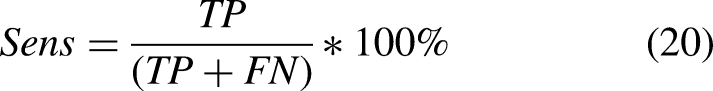
Sensitivity (Sens) provides information about the true positive percentage correctly classified during the testing process:

S e n s = \frac{T P}{(T P + F N)} * 100 %

(20)

Specificity (Spec) provides information about true negatives correctly classified during the testing process:

S p e c = \frac{T N}{(T N + F P)} * 100 %

(21)

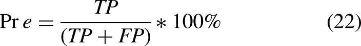
Precision (Pre) is the percentage of instances marked positive by the classifier relative to the total predicted positive (classifier accuracy):

Pr e = \frac{T P}{(T P + F P)} * 100 %

(22)

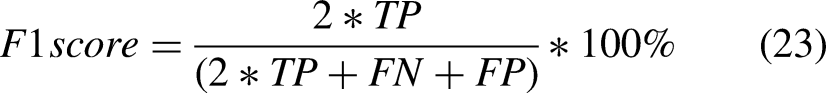
The F1 score shows the harmonic average of precision and recall:

F 1 s c o r e = \frac{2 * T P}{(2 * T P + F N + F P)} * 100 %

(23)

Diabetes risk scorecard

We have developed a risk assessment card based on a diabetes prediction model, designed to evaluate the risk of developing diabetes. In comparison to the probability outputs of machine learning models, the scorecard offers a more intuitive and interpretable approach to express risk, with increased stability. The principle is to convert the coefficients and intercepts of the diabetes prediction model into easy-to-understand scores, calculate the scores according to the patient's characteristic parameters, and finally map the scores to the corresponding risk levels. Through the use of risk assessment cards, doctors and patients can better understand the risk of diabetes and take corresponding preventive and treatment measures, thereby improving the effectiveness of diabetes prevention and treatment. The entire process involves binning, WOE transformation, feature selection, and score transformation and is described in detail as follows. See Appendix B for pseudocode.

Variable binning

Usually, the chi-squared statistic is employed to measure the class distribution between two adjacent intervals. If two adjacent intervals exhibit similar class distributions, they are merged. Otherwise, they remain separate. The specific binning process is as follows:

Continuous variables are divided into 50–100 subgroups.

Ensure each subgroup contains both diseased and healthy samples.

Utilize the chi-squared test to compare the similarity between two bins. Conduct a chi-squared test between adjacent groups and merge the two groups with the largest chi-squared test p-value until the number of groups is less than the set number of bins.

A feature is divided into several bins. Observe the changes in IV for each group of bins to determine the most suitable number of bins.

After binning, calculate the Weight of Evidence (WoE) value for each bin.

WOE encoding

WOE, short for Weight of Evidence, is the ratio of chronic disease patients to healthy individuals in the current bin and the difference in this ratio compared to the overall population. The larger the WOE, the greater the likelihood of chronic disease patients in the current group. Conversely, the smaller the WOE, the less likely the samples in this group will exhibit the response. For the i-th bin of the independent variable, the WOE value can be calculated as follows:

W O E_{i} = \ln (\frac{p_{i_{1}}}{p_{i_{0}}}) = \ln (\frac{# B_{i} / # B_{T}}{# G_{i} / # G_{T}})

(24)

p_{i_{1}}

is the proportion of chronic disease patients in the i-th bin to all chronic disease patients.

p_{i_{0}}

is the proportion of healthy individuals in the i-th bin to all healthy individuals.

# B_{i}

is the number of chronic disease patients in the i-th bin.

# G_{i}

is the number of healthy individuals in the i-th bin.

# B_{T}

is the total number of chronic disease patients.

# G_{T}

is the total number of healthy individuals.

Univariate selection based on IV values

The formula to calculate the IV value for the i-th bin of a variable is given by:

I V_{i} = (\frac{# B_{i}}{# B_{T}} - \frac{# G_{i}}{# G_{T}}) * \ln (\frac{# B_{i} / # B_{T}}{# G_{i} / # G_{T}}) = (\frac{# B_{i}}{# B_{T}} - \frac{# G_{i}}{# G_{T}}) * W O E_{i}

(25)

The IV value for the variable is the sum of the IV values for all the bins.

Conversion into a scorecard

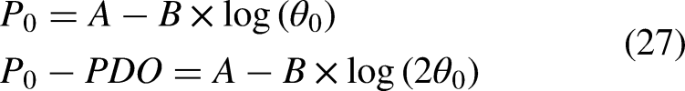
After modeling and evaluating the data following the binning process, it is necessary to transform the model into a standard scorecard. This process is referred to as the scaling of the credit scorecard. The score scale set by the credit scorecard can be calculated using the following formula:

S c o r e = A - B \times \ln (o d d s) = A - B \times θ^{T} x

(26)

In this expression, odds represent the ratio of healthy individuals to patients,

\ln (o d d s)

is the natural logarithm of the odds, which is the coefficient of LR. A and B are constants. Logistic regression is, in fact, a linear regression model with the natural logarithm of the odds as the dependent variable. The score when the odds are

θ_{0}

P_{0}

, and the score when the odds are

2 θ_{0}

P_{0} - P D O

. Substituting these values into the linear expression above, we obtain:

\begin{aligned} P_{0} = A - B \times \log (θ_{0}) \\ P_{0} - P D O = A - B \times \log (2 θ_{0}) \end{aligned}

(27)

Solving this system of equations, we can obtain the values for A and B. In practical applications, we calculate the scores corresponding to each bin for each variable. When a new user's data are available, their values for each bin are added together. Finally, the initial base score is added to get the overall result:

S c o r e = A - B {θ_{0} + θ_{1} x_{1} + \cdot \cdot \cdot + θ_{n} x_{n}}

(28)

In the equation, variable

x_{1} \dots x_{n}

represents one of the variables included in the final model. Since all the variables included in the model have undergone WOE encoding, each of these independent variables can be expressed in the form of

(θ_{i} ω_{i j}) δ_{i j}

S c o r e = A - B {\begin{matrix} θ_{0} \\ + (θ_{1} ω_{11}) δ_{11} + (θ_{1} ω_{12}) δ_{12} + \cdot \cdot \cdot \\ \cdot \cdot \cdot \\ + (θ_{n} ω_{n 1}) δ_{n 1} + (θ_{n} ω_{n 2}) δ_{n 2} + \cdot \cdot \cdot \end{matrix}}

(29)

In the equation,

A - B θ_{0}

represents the base score,

θ_{i}

is the coefficient of the i-th independent variable in LR,

ω_{i j}

is the WOE value of the j-th bin of the i-th variable,

δ_{i j}

is a 0–1 indicator variable where

δ_{i j} = 1

represents the i-th variable taking the j-th bin, and

δ_{i j} = 0

represents the i-th variable not taking the j-th bin. Finally, the scorecard is scaled to obtain a total score between 0 and 100. The final scorecard consists of the base score and the scores for each bin of each feature.

Statement

Haizhu District Community Health Development Guidance Center authorized and approved the data used in our study and waived the requirement of informed consent. All methods were carried out in accordance with relevant guidelines and regulations.

Results

Data balancing

The features of the dataset are all numerical features, and since we will use a tree based model, we will perform nonlinear scaling on features with skews greater than 0.5 among various features. In the dataset (Appendix C, Figure a), “Exercise_Time” skewness is 67.2, “Exercise_Frequency” skewness is 56.9, “Exercise_Total_Time” skewness is 49, “Staple_Food” skewness is 10.1, “Diastolic_BP” skewness is 5.8, and “BMI” skewness is 0.9. We use logarithmic scaling. The logarithmic function increases the spacing between small numbers and reduces the spacing between large numbers. When the values of certain features are densely packed in small values, by increasing these intervals, our model will increase the intervals of small values, and we can improve the performance of the model when using these values for training and testing. After scaling, it can be seen that the skewness has been greatly improved (Appendix C, Figure b). The top six skewness values are “Systolic_BP” 0.06, “BMI” 0.04, “Age” 0.02, “Exercise_Total_Time” 0.02, “Drinking” 0.01, and “Exercise_ Time” 0.01.

Draw a distribution histogram using the maximum skewness feature Systolic_BP as an example. From Appendix D, Figure (a), it can be seen that the imbalance also seems to be large. We use three oversampling methods, namely SMOTE, ADASYN, RandomOverSampler, and two undersampling methods, RandomUnderSampler and Near Miss, to balance the dataset. From Appendix F, it can be seen that the distribution of samples after oversampling is more balanced than under sampling. From Appendix D, it can be seen that among the three oversampling algorithms, RandomOverSampler has a more balanced distribution compared to SMOTE and ADASYN. From Appendix E, it can also be seen that the samples after RandomOverSampler equalization are more concentrated in terms of data distribution width. Therefore, oversampling RandomOverSampler is more suitable for us to use the equalization of the dataset. This has a certain relationship with our dataset. The number of minority class samples in the dataset is significantly small, and the distribution of samples in other categories is relatively balanced. Using RandomOverSampler can easily and quickly increase the number of minority class samples, thereby balancing the distribution of categories. In addition, there is no significant overlap between categories in the dataset, and RandomOverSampler can balance categories by copying a few class samples without introducing composite samples, avoiding the potential noise and inaccuracy that composite samples may introduce.

Characteristic selection

The dataset we adopted contains a total of 12 clinical features. We use feature selection to exclude these redundant features. We used three feature selection methods (SelectKBest with f_ANOVA-based, RFE, SelectKBest with Mutual Information) and compared the relationship between different numbers of clinical features and the AUC of RF classifiers. We varied the number of features selected from 1 to 12 and plotted AUC vs. number of features for each method, finding that all methods had the best AUC score when using eight features. The relationship between the number of feature selections and AUC is shown in Figure 1. It can be observed that after the number of feature variables reaches eight, adding more feature variables does not improve the performance of the prediction model, which also indicates that the variables outside the optimal feature parameters are redundant information or noise.

The results of feature parameter importance coefficients using three feature selection techniques are shown in Table 1. We noticed that using the eight optimal feature parameters BMI, Age, diff_BP, Systolic_BP, Diastolic_BP, Exercise_total_time, and Exercise_frequency, Smoking generated by SelectKBest with ANOVA-based can achieve an accuracy of 89.32%; using the eight optimal parameters BMI_age, BMI, Age, diff_BP, Systolic_BP, Diastolic_BP, Staple_food, and Exercise_total_time generated by RFE can achieve accuracy of 91.42%; the optimal characteristic parameters BMI_age, BMI, Age, diff_BP, Systolic_BP, Diastolic_BP, Staple_food generated by SelectKBest with Mutual Information, and Exercise_total_time can achieve accuracy of 91.42%. The confusion matrix and ROC curves using the three feature selection techniques are shown in Appendix G. The performance and results of the two optimal feature parameter selection methods of RFE and SelectKBest with Mutual Information are basically the same, and the performance is slightly better than SelectKBest with ANOVA-based. Using the RFE method requires four feature counts to achieve the highest AUC. Regardless of the feature selection technique used, the best feature subset always contained the six feature variables of BMI, Age, diff_BP, Systolic_BP, Diastolic_BP, and Exercise_total_time, indicating the importance of these features in diagnosis and prevention of diabetes (Figure 2).

Figure 2.

Results of Feature Quantity using Three Feature Selection Techniques.

Table 1.

Results of feature importance coefficients using three feature selection techniques.

SelectKBest with ANOVA-based		RFE		SelectKBest with Mutual Information
FEATURE	Importance coefficient	Feature	Importance coefficient	Feature	Importance coefficient
BMI	0.3160	BMI_age	0.1912	BMI_age	0.1912
Age	0.2136	BMI	0.1827	BMI	0.1827
diff_BP	0.1209	Age	0.1219	Age	0.1219
Systolic_BP	0.1128	diff_BP	0.1094	diff_BP	0.1094
Diastolic_BP	0.1072	Systolic_BP	0.1028	Systolic_BP	0.1028
Exercise_total_time	0.0745	Diastolic_BP	0.0992	Diastolic_BP	0.0992
Exercise_frequency	0.0354	Staple_food	0.0991	Staple_food	0.0991
Smoking	0.0197	Exercise_total_time	0.0937	Exercise_total_time	0.0937
Accuracy	0.8932	Accuracy	0.9142	Accuracy	0.9142
F1 score	0.8855	F1 score	0.9092	F1 score	0.9092

Risk assessment of diabetes

Models learned from imbalanced datasets may have poor generalization ability.^44,45 We employ a random oversampling technique for imbalanced datasets by replicating the minority class examples to balance the data. We divided the dataset into a training set and a test set in a ratio of 70–30%. By using the eight best features generated by SelectKBest with Mutual Information, we compared the performance of six different classifier models, namely RF, XGB, KNN, MLP, GBDT, and VC, and compared the performance indicators of the six models, as shown in Figure 3 and Appendix H. It can be seen that the classifier based on RF can achieve 91.41% accuracy, 93.45% precision, 88.51% recall rate, 90.91% F1 score, and 91.33% ROC performance, all indicators are higher than other five kind of model. Therefore, RF was chosen as the final algorithm. Furthermore, we utilized the research dataset, namely the prebalanced dataset, to test the trained model. The accuracy achieved was 88.94%, with a precision of 89.51%, recall of 85.56%, an F1 score of 88.27%, and an AUC of 89.78%.

Figure 3.

Confusion matrices and ROC curves for diabetes risk assessment using RF, XGB, KNN, MLP, GBDT, vc. (a) Confusion matrices using six models: RF, XGB, KNN, MLP, GBDT, and VC. (b) ROC curves using six models: RF, XGB, KNN, MLP, GBDT, and VC.

Diabetes prediction risk assessment card

By using a scorecard calculation, we computed individual diabetes risk scores to evaluate the risk level of disease. In constructing the scorecard, we initially discretized continuous variables using the quantile equal frequency method and measured the disease probability of each bin with WoE. After binning, the WoE value for each bin replaced the original data value, and LR was employed for modeling. Following modeling, we computed the scores for each bin using LR coefficients and a score formula. Finally, the relationship between the total score and the risk level was determined using a KS curve. We used the Python library toad for risk scorecard modeling. Specific steps are as follows:

According to the optimal feature selected in 2.4 as the feature column, it is stored in the train_cols_1 list.

Select the feature columns in the train_cols_1 list from the training dataset and store them in the selected_train variable. At the same time, the same feature columns as selected_train are selected from the test dataset and stored in the selected_test variable.

For the feature column in the selected_train variable, use the toad.transform.Combiner() method for binning.

For the binned data, use the toad.transform.WOETransformer() method for WOE conversion.

Use the toad.selection.stepwise() method for feature selection and use the AIC criterion and two-way search when selecting features.

Use the LogisticRegression() method for model training and perform model performance evaluation on the training set.

For the test set, use the features selected in the training set to make predictions and perform model performance evaluation on the test set.

Use the toad.metrics.PSI() method to compare whether the variable distribution of the training set and the test set is stable.

Use the toad.scorecard.ScoreCard() method to convert the score and output the converted result.

The scorecard transformation algorithm was used to convert the model into a scorecard. We set the P0 and PDO values to 2 and 60. Using the formula 26, we calculated the entire scorecard. The main feature binning results are shown in Table 2 and Appendix I. This is the final diabetes risk scorecard. The scorecard consists of base scores and corresponding scores for each bin under each feature. When a new user emerges, the score is calculated by adding the base score to the scores for each bin under each feature using the scorecard.

Table 2.

Diabetes risk scorecard.

Base_score: 750
Feature	Threshold	Score	Feature	Threshold	Score
BMI	[-inf–20.77)	63.04	diff_BP	[-inf–40.0)	53.1
	[20.77–21.72)	68.03		[40.0–44.0)	60.39
	[21.72–22.32)	61.47		[44.0–46.0)	57.7
	[22.32–22.94)	56.58		[46.0–48.0)	57.41
	[22.94–23.53)	52.88		[48.0–50.0)	56.93
	[23.53–24.22)	56.19		[50.0–52.0)	61.13
	[24.22–24.91)	58.77		[52.0–54.0)	60.62
	[24.91–25.95)	51.54		[54.0–56.0)	56.54
	[25.95–27.46)	49.19		[56.0–60.0)	52.16
	[27.46–inf)	41.97		[60.0–inf)	43.11
Staple_food	[-inf–200.0)	73.13	Exercise_total_time	[-inf–40.0)	65.45
	[200.0–250.0)	72.26		[40.0–80.0)	68.22
	[250.0–260.0)	39.23		[80.0–90.0)	49.11
	[260.0–300.0)	37.05		[90.0–120.0)	59.89
	[300.0–330.0)	53.62		[120.0–150.0)	54.68
	[330.0–350.0)	41.17		[150.0–180.0)	53.95
	[350.0–400.0)	61.6		[180.0–270.0)	47.57
	[400.0–500.0)	47.76		[270.0–inf)	40.36
	[500.0–inf)	78.53
Systolic_BP	[-inf–118.0)	55.43	Diastolic_BP	[-inf–70.0)	52.14
	[118.0–120.0)	60.61		[70.0–72.0)	64.6
	[120.0–123.0)	67.02		[72.0–74.0)	55.85
	[123.0–125.0)	63.07		[74.0–75.0)	62.17
	[125.0–128.0)	63.78		[75.0–77.0)	62.6
	[128.0–130.0)	57.91		[77.0–78.0)	41.72
	[130.0–131.0)	62.24		[78.0–80.0)	58.24
	[131.0–134.0)	51.7		[80.0–82.0)	59.51
	[134.0–136.0)	48.89		[82.0–85.0)	50.95
	[136.0–inf)	30.74		[85.0–inf)	40.57
Age	[-inf–51.0)	47	BMI_age	[-inf–1158.56)	57.81
	[51.0–55.0)	54.73		[1158.56–1273.98)	57.36
	[55.0–59.0)	49.64		[1273.98–1363.20)	56.63
	[59.0–61.0)	54.91		[1363.20–1453.28)	54.06
	[61.0–65.0)	52.05		[1453.28–1541.08)	55.95
	[65.0–69.0)	63.22		[1541.08–1636.8)	53.35
	[69.0–73.0)	48.13		[1636.8–1736.04)	52.28
	[73.0–77.0)	53.62		[1736.04–1858.08)	54.81
	[77.0–82.0)	64.84		[1858.08–2028.74)	60.9
	[82.0–inf)	69.49		[2028.74–inf)	56.21

To set the risk intervals, we employed a KS curve to describe the total score. The KS value (Kolmogorov–Smirnov value) is a metric used to evaluate the performance of classification models, typically employed to assess the performance of binary classifiers. The KS value represents the maximum difference between the true positive rate (True Positive Rate) and the false positive rate (False Positive Rate) at different probability thresholds. A higher KS value indicates a better ability of the model to distinguish different thresholds. As shown in Figures 3(d), the KS values is 0.74, respectively, suggesting a favorable model performance. The corresponding thresholds at the maximum turning point is 0.39, respectively. Hence, 0.39 was set as the intermediate threshold. For anyone undergoing the test, a lower score corresponds to a higher risk of diabetes. Conversely, a higher score indicates a lower risk of diabetes. To provide users with a more direct scoring effect, we set four score turning points at 0.2, 0.4, 0.6, and 0.8 based on the KS chart. Adding the base score to the minimum scores of each feature's corresponding bin is calculated as ScoreMin, and adding the base score to the maximum scores of each feature's corresponding bin is calculated as ScoreMax. Based on the four score turning points obtained from the KS chart, ScoreMin and ScoreMax are divided into intervals. The total score can be divided into five risk intervals, corresponding to low risk, relatively low risk, moderate risk, relatively high risk, and high risk. When a new user appears, the risk situation is determined by using the scorecard to sum the base score with the scores corresponding to the bins of each feature and identifying the risk interval of the total score.

In the process of discretizing continuous features through binning algorithms, there is inevitably an information loss. Therefore, it is necessary to assess the model's performance at this stage to determine the degree of information loss due to binning. We use the test set to verify the effectiveness of the scorecard, and the resulting confusion matrix, ROC, TPR, and FPR are shown in Figure 4(a)–(c). The experimental results show that the accuracy of the risk scorecard on the training set is 94.83%, the precision is 97.54%, the recall is 91.64%, and the F1 score is 94.50%. The accuracy of the risk scorecard on the test set is 86.70%, the precision is 89.08%, the recall is 80.34%, and the F1 score is 84.48%. Furthermore, we tested the risk scorecard on the research dataset, which is the dataset before balancing. The results were an accuracy of 85.16%, precision of 87.30%, recall of 80.26%, and an F1 score of 83.27%. It can be seen that the risk scorecard has little performance loss compared to the 3.3 model performance. This suggests that the binning method used to construct the diabetes risk scorecard is reasonable and results in very low feature information loss.

Figure 4.

Establishment of the diabetes risk assessment card model. (a) Confusion matrix of the training set for the scorecard. (b) Confusion matrix of the validation set for the scorecard. (c) ROC curve for validating the performance of the scorecard. (d) TPR (True Positive Rate), FPR (False Positive Rate), and KS curve for validating the performance of the scorecard.

Discussion

According to “Characteristic selection” section, regardless of the feature selection technique used, the optimal feature subset consistently includes six features: BMI, Age, diff_BP, Systolic_BP, Diastolic_BP, and Exercise_total_time. This indicates the importance of these features in the diagnosis and prevention of diabetes. Using the eight best features generated by the SelectKBest with Mutual Information method and the best RF classifier obtained in “Risk assessment of diabetes” section as a comparative baseline, we attempted to remove BMI_age and Staple_food, keeping only the subset of six best features. The accuracy in this case was 83.89%. Trying to remove only the most important features, BMI_age and BMI, resulted in an accuracy of 80.45%. Removing only BMI_age and Age led to an accuracy of 82.32%. Simultaneously removing the top three important features, BMI_age, BMI, and Age, resulted in an accuracy of 66.57%. The results are presented in Appendix J, showing that compared to the optimal features with an accuracy of 86.94% in “Risk assessment of diabetes” section, the model's performance significantly decreases when key features are removed, indicating that the amalgamation of features provides richer information and better comprehensive judgment of diabetes risk. The integration of various features enhances the robustness, reliability, and accuracy of the proposed diabetes diagnostic model.

We further analyzed the distribution of typical diabetes features, providing a detailed presentation of the differences between diabetes patients and healthy individuals, as shown in Appendix K. Apart from the features Staple_food and Exercise_total_time, all other features exhibit significant statistical differences. Individual BMI, age, and blood pressure are closely associated with diabetes, being the most crucial risk factors. The risk of an individual developing diabetes demonstrates an association with BMI, age, and blood pressure levels. As BMI increases, the risk of diabetes gradually rises. With advancing age, the risk of the disease also increases. Additionally, elevated blood pressure levels are closely linked to the onset of diabetes. To effectively prevent and control diabetes, it is essential to gain a profound understanding of these critical features and risk factors associated with the disease.

In this context, community-based diabetes prevention and control efforts become particularly crucial. By strengthening preventive measures and interventions at the community level, we can enhance residents’ health awareness and guide them in better managing their personal health. This includes encouraging the adoption of positive lifestyle choices, such as maintaining a balanced diet and engaging in moderate exercise to slow down the increase in BMI. Furthermore, through health education activities, we can better convey information about diabetes, raising the community's awareness of the disease. Individual self-health management is a crucial aspect of preventing diabetes. Through self-examination, individuals can promptly detect changes in their bodies and take corresponding measures. Additionally, encouraging individuals to proactively adjust their lifestyles, including quitting smoking, moderating alcohol consumption, and ensuring adequate sleep, contributes to reducing the risk of developing diabetes.

In summary, community-based diabetes prevention and control efforts require a comprehensive approach, aiming to reduce the incidence of the disease at its source. Through the collective efforts of society, we can effectively improve the lifestyle of community residents, enhance overall health levels, and reduce the risk of developing diabetes.

While this study has made significant strides, it is not without notable limitations, one of which is the insufficient comprehensiveness of the features, potentially impacting the accurate prediction of disease risk. Nonetheless, we maintain a positive outlook on the methods proposed in the study and the predictive model employed. We believe that training and predicting with a more extensive and comprehensive set of features are not only feasible but also likely to further enhance the predictive accuracy of the model.

In future in-depth investigations, we are committed to extracting more extensive and comprehensive feature variables to explore the key factors influencing disease risk from a more holistic perspective. We plan to employ time-series analysis on follow-up data to delve deeper into variables associated with blood sugar improvement, providing better guidance for the self-health management of patient populations. Additionally, we will focus on the importance of early prediction of diabetes complications, with future work exploring the extraction of more data related to diabetes complications to study preventive strategies. This series of efforts aims to continuously refine our research framework, ensuring its better alignment with the practical needs of disease management and prevention.

Conclusions

Based on the method of feature selection and risk scorecard, we modeled the real follow-up data of diabetic patients obtained from the grassroots community service management information system in Haizhu District, Guangzhou City, and assessed the risk of diabetes. Firstly, three oversampling methods and two undersampling methods were used to balance the dataset. Through visual analysis, the oversampling technique RandomOverSampler was selected as the equalization algorithm. Subsequently, three feature selection methods were used to screen and optimize the relevant features of diabetes, and the optimal subset of features associated with community follow-up and diabetes risk was determined, which can be used as a key physiological feature for diabetes patients to focus on. The WOE conversion method is used to convert the features, and the quantile sub box method is used to discretization the converted features, the discretized features are transformed into scores that are easy to understand and explain, and the patient's risk is classified into different levels based on the scores. Finally, the effectiveness and reliability of this method in diabetes risk assessment were demonstrated by comparing the predictive performance of different models. The risk assessment model and scoring card can be directly applied to large-scale risk identification and warning by community doctors, as well as for patients to conduct self-examination and targeted improvement of their lifestyle, reducing the level of risk factors. The research results of this paper provide strong support for diabetes risk prediction and clinical practice and provide new ideas and methods for research in related fields.

Footnotes

Acknowledgments

The authors would like to forward our deepest gratitude to the Haizhu District Community Health Development Guidance Center, the research data management unit.

Contributorship

Liangjun Jiang conceived and designed this study and wrote the manuscript. Donghai Wang and Juan Li analyzed and explained the data. Zerui Yang conducted code design. Haimei Gong and Jing Wang assisted in literature search. Lei Wang conducted research supervision and made key revisions to the manuscript. All authors have read and agreed to the published version of the manuscript.

Data availability statement

The datasets analyzed during the current study are not publicly available due to privacy but are available from the corresponding author on reasonable request.

Declaration of conflicting interests

The authors declared no potential conflicts of interest with respect to the research, authorship, and/or publication of this article.

Ethical approval

Funding

This work was supported by the Hainan Province Science and Technology Special Fund(ZDYF2022SHFZ026), the National Natural Science Foundation of China(62163010).

Guarantor

ORCID iD

Lei Wang

Appendix A

Algorithm 1.

Feature selection.

Appendix B

Algorithm 2.

Diabetes Risk Scorecard.

Appendix C

Appendix D

Appendix E

Appendix F

Appendix G

Appendix H

Table.

Comparison of performance metrics for the models.

Methods	Accuracy (%)	Precision (%)	Recall (%)	F1_score (%)	ROC (%)
RF	91.41	93.45	88.51	90.91	91.33
XGB	69.17	69.65	64.59	67.03	69.03
KNN	72.32	75.79	63.09	68.86	72.05
MLP	59.11	58.03	56.77	57.40	59.04
GBDT	58.73	59.35	47.39	52.70	58.40
VC	83.64	88.45	76.24	81.89	83.43

Appendix I

Appendix J

Table.

Performance after removing important features.

	Accuracy (%)	Precision (%)	Recall (%)	F1_score (%)	ROC (%)
Delete BMI_age & Staple_food	83.89	88.84	83.63	86.09	87.77
Delete BMI_age & BMI	80.45	86.19	78.66	82.16	84.29
Delete BMI_age & Age	82.32	88.35	80.59	84.19	86.15
Delete BMI_Age, BMI, Age	66.57	71.43	62.07	66.28	70.32

Appendix K

References

Evwiekpaefe

Abdulkadir

. A predictive model for diabetes mellitus using machine learning techniques (A study in Nigeria). African J Inf Syst 2023; 15: 1.

Mansoori

Sahranavard

Hosseini

, et al. Prediction of type 2 diabetes mellitus using hematological factors based on machine learning approaches: a cohort study analysis. Sci Rep 2023; 13: 663.

Rastogi

Bansal

. Diabetes prediction model using data mining techniques. Meas Sens 2023; 25: 100605.

Doğru

Buyrukoğlu

Arı

. A hybrid super ensemble learning model for the early-stage prediction of diabetes risk. Med Biol Eng Comput 2023; 61: 785–797.

Jaber

James

. Early prediction of diabetic using data mining. SN Comput Sci 2023; 4: 169.

Wild

Roglic

Green

, et al. Global prevalence of diabetes: estimates for the year 2000 and projections for 2030. Diabetes Care 2004; 27: 1047–1053.

Rydén

, et al. Guidelines on diabetes, pre-diabetes, and cardiovascular diseases: executive summary: the task force on diabetes and cardiovascular diseases of the European Society of Cardiology (ESC) and of the European Association for the Study of Diabetes (EASD). Eur Heart J 2007; 28: 88–136.

Engelgau

Narayan

Herman

. Screening for type 2 diabetes. Diabetes Care 2000; 23: 1563–1580.

Rolka

Venkat Narayan

Thompson

, et al. Performance of recommended screening tests for undiagnosed diabetes and dysglycemia. Diabetes Care 2001; 24: 1899–1903.

10.

Ahmed

, et al. Prediction of diabetes empowered with fused machine learning. IEEE Access 2022; 10: 8529–8538.

11.

Khan

Zeb

Al-Rakhami

, et al. Detection and prediction of diabetes using data mining: a comprehensive review. IEEE Access 2021; 9: 43711–43735.

12.

Polat

Güneş

. An expert system approach based on principal component analysis and adaptive neuro-fuzzy inference system to diagnosis of diabetes disease. Digit Signal Process 2007; 17: 702–710.

13.

Liu

Valdez

, et al. Application of support vector machine modeling for prediction of common diseases: the case of diabetes and pre-diabetes. BMC Med Inform Decis Mak 2010; 10: 16.

14.

Bukhari

Alkhamees

Hussain

. An improved artificial neural network model for effective diabetes prediction. Complexity 2021; 2021: 5525271.

15.

Hasan

Alam

Das

, et al. Diabetes prediction using ensembling of different machine learning classifiers. IEEE Access 2020; 8: 76516–76531.

16.

Larabi-Marie-Sainte

Aburahmah

Almohaini

, et al. Current techniques for diabetes prediction: review and case study. Appl Sci 2019; 9: 4604.

17.

Alam

Iqbal

Ali

, et al. A model for early prediction of diabetes. Inform Med Unlocked 2019; 16: 100204.

18.

López

Torrent-Fontbona

Viñas

, et al. Single nucleotide polymorphism relevance learning with random forests for type 2 diabetes risk prediction. Artif Intell Med 2018; 85: 43–49.

19.

Zou

Luo

, et al. Predicting diabetes mellitus with machine learning techniques. Front Genet 2018; 9: 515.

20.

Dinh

Miertschin

, et al. A data-driven approach to predicting diabetes and cardiovascular disease with machine learning. BMC Med Inform Decis Mak 2019; 19: 211.

21.

Han

Y-M

Yang

Huang

Q-L

, et al. Risk prediction of diabetes and pre-diabetes based on physical examination data. Math Biosci Eng 2022; 19: 3597–3608.

22.

Phongying

Hiriote

. Diabetes classification using machine learning techniques. Computation 2023; 11: 96.

23.

Griffin

Little

Hales

, et al. Diabetes risk score: towards earlier detection of type 2 diabetes in general practice. Diabetes Metab Res Rev 2000; 16: 164–171.

24.

Kanaya

Fyr

CLW

De Rekeneire

, et al. Predicting the development of diabetes in older adults: the derivation and validation of a prediction rule. Diabetes Care 2005; 28: 404–408.

25.

Mohan

Deepa

, et al. A simplified Indian Diabetes Risk Score for screening for undiagnosed diabetic subjects. J Assoc Physicians India 2005; 53: 759–763.

26.

Lindstrom

Tuomilehto

. The diabetes risk score: a practical tool to predict type 2 diabetes risk. Diabetes Care 2003; 26: 725–731.

27.

Lei

Tingtao

Jianan

, et al. Transformer fault diagnosis strategy considering parameter optimization of oversampler and classifier. Electr Power Autom Equip 2023; 43: 209–217.

28.

Laicun

. Skewness of data distribution: measurement methods and software calculation. Stat Decis 2022; 14: 30–33.

29.

Bing-fu

JIN

. Influencing factors and significance of the skewness coefficient in grain size analysis. Marine Sci 2012; 36: 129–135.

30.

Chawla

Bowyer

Hall

, et al. SMOTE: synthetic minority over-sampling technique. J Artif Intell Res 2002; 16: 321–357.

31.

Bai

Garcia

, et al. ADASYN: Adaptive synthetic sampling approach for imbalanced learning. Neural Networks, 2008. IJCNN 2008. (IEEE World Congress on Computational Intelligence). IEEE International Joint Conference on IEEE, 2008.

32.

Ahmad

Mukhtar

Alaqail

, et al. Investigating health-related features and their impact on the prediction of diabetes using machine learning. Appl Sci 2021; 11: 1173.

33.

Maniruzzaman

Rahman

Ahammed

, et al. Classification and prediction of diabetes disease using machine learning paradigm. Health Inf Sci Syst 2020; 8: 7.

34.

Tripathi

Kumar

. Early prediction of diabetes Mellitus using machine learning. 2020 8th International Conference on Reliability, Infocom Technologies and Optimization (Trends and Future Directions) (ICRITO), Noida, India. 2020;1009–1014.

35.

Abdollahi

Nouri-Moghaddam

. Hybrid stacked ensemble combined with genetic algorithms for diabetes prediction. Iran J Comput Sci 2022; 5: 205–220.

36.

Patil

Tamane

. A comparative analysis on the evaluation of classification algorithms in the prediction of diabetes. Int J Electr Comput Eng (IJECE) 2018; 8: 3966–3975.

37.

Pham

, et al. A novel wrapper–based feature selection for early diabetes prediction enhanced with a metaheuristic. IEEE Access 2021; 9: 7869–7884.

38.

Singh

Dhillon

Kumar

, et al. eDiaPredict: an ensemble-based framework for diabetes prediction. ACM Trans Multimed Comput Commun Appl 2021; 17: 1551–6857.

39.

Ramesh

Aburukba

Sagahyroon

. A remote healthcare monitoring framework for diabetes prediction using machine learning. Healthc Technol Lett 2021; 8: 45–57.

40.

Selvakumar

Senthamarai Kannan

GothaiNachiyar

. Prediction of diabetes diagnosis using classification based data mining techniques. Int J Stat Syst 2017; 12: 183–188.

41.

Prabhu

Selvabharathi

. Deep belief neural network model for prediction of diabetes mellitus. 2019 3rd International Conference on Imaging, Signal Processing and Communication (ICISPC), Singapore. 2019:138–142.

42.

Kumari

Kumar

Mittal

. An ensemble approach for classification and prediction of diabetes mellitus using soft voting classifier. Int J Cogn Comput Eng 2021; 2: 40–46.

43.

Rajendra

Latifi

. Prediction of diabetes using logistic regression and ensemble techniques. Comput Methods Prog Biomed Update 2021; 1: 100032.

44.

Huang

Yin

, et al. Diabetes Mellitus risk prediction using age adaptation models. Biomed Signal Process Control 2023; 80: 104381.

45.

Nnamoko

Korkontzelos

. Efficient treatment of outliers and class imbalance for diabetes prediction. Artif Intell Med 2020; 104: 101815.

Diabetes prediction model for unbalanced community follow-up data set based on optimal feature selection and scorecard

Abstract

Objectives

Methods

Results

Conclusion

Keywords

Introduction

Materials and methods

System design

Patients and data sets

Data balancing processing

Skewness

Synthetic minor oversampling technique

Adaptive synthetic sampling

RandomOverSampler

RandomUnderSampler

Near Miss

Characteristic selection of diabetes

Selectkbest with ANOVA-based

Recursive feature elimination

SelectKBest with mutual information

Classification algorithm

Random forest

Gradient boosting decision tree

eXtreme Gradient Boosting

K-Nearest neighbors

Multilayer perceptron

Ensemble learning

Statistical analysis metrics used for model evaluation

Diabetes risk scorecard

Variable binning

WOE encoding

Univariate selection based on IV values

Conversion into a scorecard

Statement

Results

Data balancing

Characteristic selection

Risk assessment of diabetes

Diabetes prediction risk assessment card

Discussion

Conclusions

Footnotes

Acknowledgments

Contributorship

Data availability statement

Declaration of conflicting interests

Ethical approval

Funding

Guarantor

ORCID iD

Appendix A

Appendix B

Appendix C

Appendix D

Appendix E

Appendix F

Appendix G

Appendix H

Appendix I

Appendix J

Appendix K

References