Sage Journals: Discover world-class research

Abstract

Lung cancer is the second foremost cause of cancer due to which millions of deaths occur worldwide. Developing automated tools is still a challenging task to improve the prediction. This study is specifically conducted for detailed posterior probabilities analysis to unfold the network associations among the gray-level co-occurrence matrix (GLCM) features. We then ranked the features based on t-test. The Cluster Prominence is selected as target node. The association and arc analysis were determined based on mutual information. The occurrence and reliability of selected cluster states were computed. The Cluster Prominence at state ≤330.85 yielded ROC index of 100%, relative Gini index of 99.98%, and relative Gini index of 100%. The proposed method further unfolds the dynamics and to detailed analysis of computed features based on GLCM features for better understanding of the hidden dynamics for proper diagnosis and prognosis of lung cancer.

Keywords

Machine learning small cell lung cancer non-small cell lung cancer (NSCLC)Cluster Prominence Bayesian method

Introduction

Lung cancer is the second leading cause of cancer and recent statistics of 2018 shows approximately 234,030 new cases of lung cancer are anticipated to be detected out of which 85% will be non-small cell lung cancer (NSCLC).^1,2 The methods of ablation and stereotactic body radiotherapy and radiofrequency are used to detect NSCLC. Small cell lung carcinoma (SCLC) and NSCLC are two main types of lung cancer, which require more powerful tools to predict, properly diagnose, and different methods of treatment. NSCLC is more common and slowly grows. Where SCLC is produced due to smoking, grows very quickly, and forms tumor in the whole body. Cancer deaths are related to a total number of cigarettes smoked.³ Lung cancer symptoms can be caused by a variety of reasons, one of which is smoking; therefore, active smokers are at a greater risk of acquiring lung cancer. Other variables that can influence the growth of lung cancer in the body include genes or a family history of lung cancer, working in an environment with dangerous compounds that can cause lung damage, and exposure to air pollution such as automobile and manufacturing fumes (Zakariya, 2014). Many distinct concepts and approaches have been proposed by various researchers. They also attempted to include image processing and machine learning techniques. Physicians are unlikely to recommend a biopsy for diagnosis unless there is clear evidence of lung cancer. Lung cancer can only be cured if earlier discovered. Lung cancer can be diagnosed using different technologies, including X-ray, magnetic resonance imaging (MRI), isotope, and computer tomography (CT). Chest X-ray (CXR) radiography and CT are two well-known anatomic imaging modalities commonly used to diagnose various lung illnesses.⁴

Lung cancer can be diagnosed with radiographic projections such as the CXR. So far, reliable computer-assisted diagnosis and data-science-based diagnosis have been deemed crucial. However, more research is being conducted to improve accuracy and imaging. Computer tomography images are superior to X-rays for RCAD lung cancer identification. The researchers concluded that using CT images in computer-assisted diagnosis systems can improve the resilience of computer-aided diagnostic (CAD) systems because X-rays have a lot less features to take out and evaluate for further processing in the direction of lung cancer detection.⁵ The CT scan is the best option for lung cancer patients because it provides detailed information on abnormal pulmonary tissues and tumors, including size, shape, and location. For a complete lung cross-section, CT scanners typically provide almost 300 scans in a short scan time. A new CAD method for the automatic detection of lung nodules in CT images is proposed in this work. The creation of a better diagnostic CAD system will enable clinicians to evaluate CT scan pictures more accurately and in less time.⁶

In the past, researchers utilized traditional machine learning algorithms. However, a more comprehensive analysis to determine the associations and other Bayesian measures to further strengthen our analysis to unfold the hidden dynamics for further improving lung cancer prediction. The parametric information from the data in recent studies has been investigated using a probabilistic propagation algorithm (Bayes Rule) by applying Bayesian networks (BNs). The degree of uncertainty and associations of variables varies from different sources such as numerical data, empirical data, and expert opinion to capture the conditional dependencies of a variable upon others.⁷ BNs have successfully been utilized in many studies by different researchers such as Kocian et al.,⁸ Amaral et al.,⁹ Laurila-Pant et al.,¹⁰ and Zhang et al.¹¹ The Bayesian inference (BI) approach utilizing the BayesiaLab has gained its popularity to investigate the causal relationships, dynamic profile analysis, target analysis, posterior probability analysis, etc. in variety of different applications including empirical analysis of brain tumor MRIs,¹² dynamic profile analysis of congestive heart failure,¹³ environmental sustainability indicators to manufacture,¹⁴ dynamical analysis of particulate matters future challenges monitoring and evaluations,¹⁵ predicting childhood lead exposure risk from community water system using Bayesian approach,¹⁶ etc. There are many applications of BI approach such as intrahepatic cholangiocarcinoma patients’ microvascular invasion,¹⁷ human factor analysis for sustainable hazardous cargo port operations,¹⁸ gallbladder polyps with malignant potential based on preoperative ultrasound Bayesian prediction analysis,¹⁹ decision-making,²⁰ industries 4.0 technologies selection,²¹ transport vulnerability,²² etc.

The causal relationships can be studied between variables that compute the probabilities of a variable when other variables in the model are known. Moreover, the Monte Carlo analysis can be used at a random sampling of probability distribution functions to denote the inputs of Bayesian model to produce hundreds or thousands of possible outcomes.²³ Recently, BNs have been utilized successfully in many applications ranging from predicting energy crop yield,²⁴ coffee rust disease prediction by employing BNs,²⁵ sustainable planning and management decision,²⁶ etc. The BNs computed the interrelation among variables that impact climate change scenarios in agriculture.²⁷ Moreover, recently, Lu et al.²⁸ utilized BNs to investigate the complex causal interactions between environments and plant diseases. Previous studies did not focus on the association among features to further unfold nonlinear dynamics in order to further diagnosis and prognosis of lung cancer.

In the present study, we aimed to apply the BI approach for comprehensive analysis to unfold the nonlinear and hidden dynamics present in the nonlinear and nonstationary lung cancer types. Lung cancer types have very severe health impact, so there is a dire need to unfold nonlinear hidden dynamics and associations among extracted features based on Bayesian artificial intelligence methods so that concerned health professional can take precautionary measures to reduce the mortality risks. We computed the associations and their strength among gray-level co-occurrence matrix (GLCM) features. The BI evaluates the posterior which can be yielded from a weighted combination of local estimates known as likelihood and estimates in surrounding spatial units. Researchers are developing intelligent methods based on machine learning algorithms that require the extraction of the most relevant features. Our research objective was multifold, first, we computed the multimodal features based on time domain, frequency domain, and entropy-based complexity measures. We then ranked the features based on t-test value. The higher the t-value indicates the more important the feature. Secondly, once we ranked the features, we then selected the high-ranked feature as our target node and then we further computed the detailed Bayesian analysis with other features to further unfold underlying hidden dynamics. We computed the relationship analysis among the extracted nodes using mutual information (MI), Kullback–Leibler (KL) divergence, and Pearson's correlation. The strength of relationship was computed using arc analysis with 3D mapping. We then computed the parent–child relationship and nodes force between the nodes. The association graph for segment profile analysis was computed for further analysis. Moreover, the network performance and significance of prominence were computed using tornado diagram. The flow of our work is presented in Figure 1. We first took lung cancer as an input signal. We then extracted the GLCM features. We then applied the features to BN and utilized different methods for detailed analysis. Finally, the network performance was evaluated using different metrics.

Figure 1.

Schematic diagram to compute the Bayesian dynamics on gray-level co-occurrence matrix (GLCM)-based features.

The Bayesian approach recently gains its popularity and utilized in many medical, signal, and image processing problems. We first computed the features considering multiple aspects in order to capture the diverse dynamics of lung cancer MRIs. We then ranked the features based on t-test, which feature sets are more important. The Cluster Prominence was set as our target node for further detailed analysis. To unfold the deeper dynamics of computed features, we can further compute the strengths of correlations, associations, strengths of target nodes and its correlation with other nodes using target profiling, and associations of target node with other nodes. This study will be very helpful to understand the deeper insights to further investigate the hidden dynamics in the signals and can play a vital role in providing an improved diagnostic system.

Materials and methods

Dataset

A publicly available dataset from www.giveascan.org was taken which is detailed and recently used in Hussain et al.²⁹ These data contain 76 patients with SCLC subjects of 563 and NSCLC of 356.

Feature extraction

The most important step in machine learning is the extraction of the relevant hand-crafted features. The features can help to improve the classification performance. In the past, researchers computed features based on different variations including texture, shape-based, geometric, and complex dynamics.^29–34 In this study, we computed GLCM-based features. GLCM features proposed by Haralick and Shanmugam³⁵ in 1973 based on texture properties. We extracted the GLCM texture features from lung MRIs developed in MATLAB and utilized them in many recent renowned studies for texture analysis.^36–39 We extracted 22 GLCM features from lung MRIs. There are various GLCM features that can be calculated, such as contrast, correlation, energy, homogeneity, and entropy. However, not all features are equally informative, and some of them may be redundant or highly correlated with others. Therefore, it is often useful to select a subset of features that are most relevant for a particular task, such as classification or segmentation.

In the context of feature selection, BayesiaLab is used to identify the most informative and relevant features for a given task. This is typically done by constructing a BN model that captures the conditional dependencies between the features and the target variable, and then using probabilistic inference techniques to estimate the marginal and conditional probabilities of the features. The final most relevant selected features were 10 returned by the BayesiaLab.

Feature importance ranking algorithms

The feature importance ranking (FIR) is used to rank the importance of features using supervised ranking algorithms.⁴⁰ The FIR algorithms developed in MATLAB were utilized.⁴¹ The importance of the extracted features was computed based on the entropy values. Entropy is used in many applications of medical systems to compute the nonlinear dynamical measures present in these systems. The higher the entropy values indicate the more complex systems with interacting components. Multiple interacting modules of biological systems produce biological signals, which show different arrangements in a complex rhythm. Due to structural part malfunctions and decreased interactions in coupling functions, these rhythms and patterns are disrupted.

T-test method for feature ranking

The t-test is a statistical hypothesis test that is used to determine whether the means of two groups of data are significantly different from each other. In the context of feature ranking, the t-test can be used to compare the means of a particular feature across groups of data and to determine whether the feature is significantly associated with the target variable. MATLAB has developed a diagnosticFeatureDesigner by providing 30 FIR methods. Based on the present data, we utilized the t-test method which is built-in in fir_mat_ttest () method which sorts the features based on the class separability criteria of two-sample t-test.⁴² The t-test method is used to rank features based on their ability to discriminate between different groups and classes of data.

The procedure for the t-test in the Diagnostic Feature Ranking Tool may involve the following steps:

Partition the dataset into two or more groups based on the target variable or class labels;

Calculate the mean and standard deviation of each feature for each group;

Calculate the t-value for each feature, which measures the difference between the means of the groups relative to the standard deviation and sample size;

Calculate the p-value for each feature, which measures the probability of obtaining the observed t-value or a more extreme value if the null hypothesis (i.e., no difference between the means) is true;

Rank the features based on their t-values or p-values, with higher values indicating greater discriminatory power.

By ranking the features based on their t-test results, the Diagnostic Feature Ranking Tool can identify the most relevant and informative features for a given classification problem.

Bayesian network analysis

Our main focus is to compute the association and relationship strength between extracted GLCM features using BI approach which is a directed acyclic graph (DAG).⁴³ Consider X = {X₁, X₂, X₃, ……X_n} a set of m dimensional variables, the couplet $X = ⟨ G, P ⟩$ a BN, where G is a DAG network and P as a set of parameters to quantify network containing each probability of the possible value of xi for each variable Xi. Mathematically:

P (X) = P (X_{1}, X_{2}, X_{3} \dots \dots ., X_{n}) = \prod_{i = 1}^{n} P (\frac{X_{i}}{X_{j (i)}})

Here,

X_{j (i)}

denotes set of parent variables of

X_{i}

for direct acyclic graph G. The posterior probabilities are thus computed using inference of variable of interest using this algorithm. We used BayesiaLab V10 for statistical analysis.⁴⁴ The Shannon entropy is computed as

H (X) = - \sum_{x ϵ X} p (X) \log_{2} p (X)

The difference between the marginal entropy and conditional entropy was computed using MI,⁴⁵ mathematically:

M I (X, Y) = H (X) - H (\frac{X}{Y})

which equals to:

M I (X, Y) = \sum_{x ϵ X} \sum_{y ϵ X} p (X, Y) \log_{2} \frac{p (X, Y)}{p (X) p (Y)}

Moreover, conditional MI (CMI) is defined as:

C M I (X, Y | Z) = \sum_{x ϵ X} \sum_{y ϵ X} \sum_{y | z ϵ X} p (X, Y | Z) \log_{2} \frac{p (X, Y | Z)}{p (X | Z) p (Y | Z)}

The p (X, Y) indicates joint probability distribution of X and Y. Whereas p(X) and p (Y) represent a marginal distribution of X and Y, respectively. The relevant Gaussian distribution of co-variance matrix variables X₁, X₂, X₃, …. X_n⁴⁶ can be computed as:

H (X) = \log (2 π e)^{\frac{n}{2}} | C |^{\frac{- 1}{2}}

The MI and CMI2 after mathematical transformation is:

M I (X, Y) = \frac{1}{2} \log \frac{| C (X) | \times | C (X) |}{| C (X, Y) |}

To correct the under estimation of CM1,⁴⁷ the CMI2 is used to integrate the interventional probability.

Statistical analysis

We computed the GLCM features from lung cancer NSCLC and SCLC MRIs using MATLAB. We then provided the feature matrix to BayesiaLab for further detailed analysis. We conducted the analysis using BayesiaLab 11.0. We used the BayesiaLab available at (https://www.bayesia.com/home/en-us/) with minimum description length (MDL) of the candidate network in its score-based algorithm to compare the BN structure.⁴⁸ The statistical independence test (GKL-test; p > 0.05) was used to validate the connections among the descriptors which were identified by the learning algorithm. The p-values or independence probabilities were utilized to check the significance of each individual relationship between the nodes or between nodes and the target node.^49,50

Exploratory analysis of the unsupervised network

The exploratory analysis can be utilized to determine the potential relationship between variables of interest.⁵¹ We can further explore the global analysis of problem of interest by computing the influence between nodes and the influence of nodes under investigation. We build our model by learning an unsupervised learning algorithm utilizing maximum spanning tree (MWST) algorithm approach developed in BayesiaLab V10.⁵² We also computed MWST. The lowest value of MDL denotes the best trade-off between complexity and data representation.

Sensitivity analysis

A detailed sensitivity analysis was performed to check the relationship among the nodes in the selected network. To understand the relationship between the nodes, we computed the highest and lowest values PM, MI, and KL, and node force between the nodes was examined globally on the network. The probabilistic dependencies were computed using MI between the nodes in the network. The tornado plots are used to display the influential knowledge of each node using sensitivity analysis on the probability of each descriptor and maximum strength of the individual relationship between the nodes and descriptors was computed. The lowest and highest probability values are displayed from the tornado plots to achieve the each node from hard evidence placed on the corresponding descriptor state. The confidence and consistency level of the sensitivity analysis using the BN model are verified by validating the model^53–55 to verify different conditions.

Segment profile analysis of energy

The analysis was also done using segment profile analysis using Radar chart for normalized mean values conditionally to Cluster Prominence for all other GLCM features. The significance was tested using Bayesian test (Best) and NHST t-test (a frequentist test). Using NHST t-test, the two-tailed t-test is utilized for null hypothesis significance testing. The Bayesian (Best test) is detailed by Kruschke⁵⁶ which follows the student's t-distribution. Moreover, 95% confidence interval is utilized. When the mean values are estimated as significant, a square is added next to the Label.

Results

In this study, we first extracted the GLCM features from lung cancer NSCLC and SCLC MRIs. The features were ranked using t-test. The highest t-test values were yielded using Cluster Prominence, and we kept it as our target node. The rest of the analysis is performance with Cluster Prominence.

Figure 2 shows the ranking of GLCM features ranked using t-test. The features are ranked without utilizing any unsupervised or supervised machine learning algorithm. A specific method that ranks the features is based on the assigned score values.⁴⁰ Finally, based on these scores, the features are ranked and the features with redundant information are further eliminated for classification. In this study, we ranked the features developed in MATLAB diagnostic tool.

Figure 2.

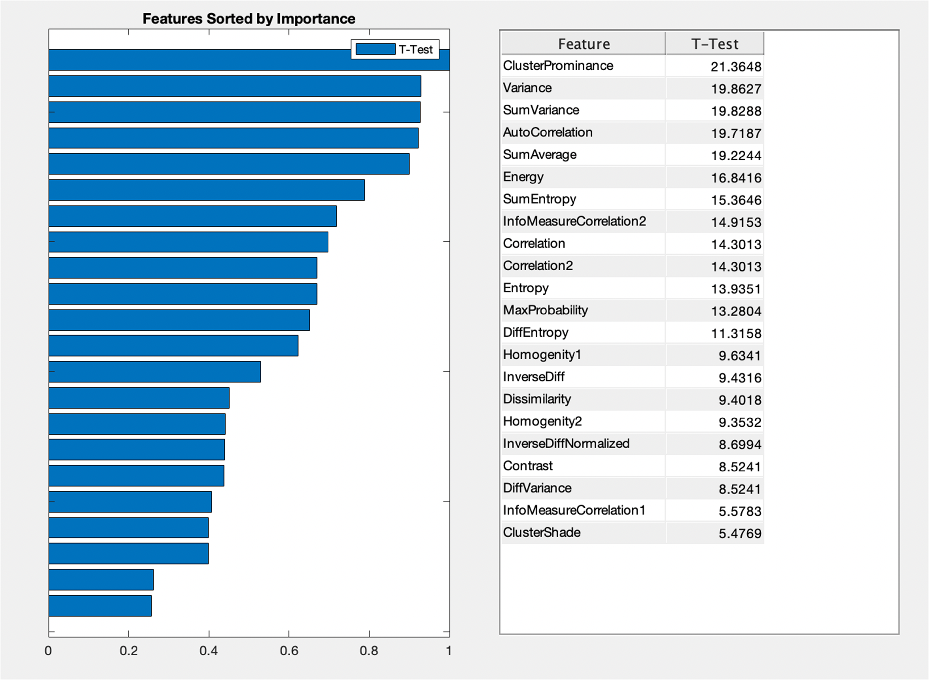
Feature ranking based on T-test values.

Figure 3 depicts the relationship analysis using BI methods including the MI, KL, and PC. The bold lines represent the stronger relationship, and the lighter lines indicate the smaller relationship. The blue color indicates the positive relationship, whereas the red color indicates the negative relationship. Moreover, the arrows indicate the $(p a r e n t \to c h i l d)$ relationship. We kept our target node as Cluster Prominence, using MI, there probability of occurrence for the state ≤330.88 (6.93%), state≤0.714.92 (30.28%), state≤1004.87 (24.33%), and state > 1004.87 (38.46%), with joint probability for all states is 100%. The probability distribution with other extracted nodes at selected states is depicted in Figure 3 (a-c).

Figure 3.

Relationship analysis using different Bayesian inference approaches such as (a) Mutual information (MI), (b) Kullback–Leibler (KL) divergence, and (c) Pearson's correlation by applying the unsupervised learning using maximum spanning tree and selecting Cluster Prominence as our target node.

Figure 4 represents the 3D mapping arc analysis to show the relationship among the multimodal extracted features. The nodes represent the features and lines represent the relationship between the nodes. The strength of relationship is denoted by the width of line. The blue color represents the positive relationship, whereas the red color denotes the negative relationship. Using the MI, the highest association was obtained between the nodes between the nodes $(C o r r e l a t i o n \to C o r r e l a t i o n 2, 1.6997)$ followed by $(e n e r g y \to e n t r o p y, 1.1536)$ , $(c l u s t e r p r o m i n a n c e \to c l u s t e r s h a d e, 0.6704)$ , and so on as reflected in Figure 4 (a). Figure 4 (b) shows the association between the nodes using KL. The highest strength of relationship was yielded between the nodes $(C o r r e l a t i o n \to C o r r e l a t i o n 2, 1.6997)$ followed by $(e n e r g y \to e n t r o p y, 1.2024)$ , $(c l u s t e r p r o m i n a n c e \to c l u s t e r s h a d e, 0.9592)$ , and so on. Figure 4 (c) denotes the relationship between nodes using Pearson's correlation. The highest relationship was yielded between the nodes $(C o r r e l a t i o n \to C o r r e l a t i o n 2, 0.9997)$ followed by $(c l u s t e r p r o m i n a n c e \to c l u s t e r s h a d e, 0.6313)$ , and so on. The highest negative relationship was yielded between the nodes $(E n e r g y \to e n t r o p y, - 0.8705)$ . The strength of relationship using these methods is also reflected in Table 1. Moreover, the highly significant results (p < 0.005) were yielded for all $(P a r e n t \to c h i l d)$ relationships except the last two pairs.

Figure 4.

Arc analysis 3D mapping to determine the relationship among the nodes (a) Mutual information, (b) Kullback–Leibler (KL) divergence, and (c) Pearson's correlation.

Table 1.

Parent–child relationship on extracted multimodal features to distinguish the NSCLC from SCLC using mutual information (MI), Kullback–Leibler (KL) divergence and Pearson's correlation.

Parent	Child	KL Divergence	Relative weight	Overall contribution	Mutual information	Pearson's correlation
Correlation	Correlation2	1.6997	1.0000	17.96%	1.6997	0.9994
Energy	Entropy	1.2024	0.7074	12.70%	1.1536	−0.8705
Cluster Prominence	Cluster shade	0.9592	0.5643	10.14%	0.6704	0.6313
Homogenity1	Dissimilarity	0.8958	0.5270	9.46%	0.8958	−0.8716
Correlation2	AutoCorrelation	0.7872	0.4631	8.32%	0.7872	0.5629
AutoCorrelation	Energy	0.6436	0.3786	6.80%	0.6436	−0.6685
AutoCorrelation	Cluster shade	0.6426	0.3781	6.79%	0.3538	−02851
Correlation2	Cluster Prominence	0.5538	0.3258	5.85%	0.4102	0.3911
Entropy	Homogenity1	0.5343	0.3143	5.64%	0.8447	−0.787
Energy	Cluster Prominence	0.4034	0.2373	4.26%	0.2599	−0.2010
Dissimilarity	Contrast	0.3908	0.2299	4.12%	0.3469	0.7623
Cluster Prominence	Contrast	0.2844	0.1673	3.00%	0.2406	0.3356
Cluster shade	Entropy	0.2749	0.1617	2.90%	0.2261	−0.0.644
AutoCorrelation	Homogenity1	0.1899	0.1117	2.00%	0.5003	−0.4982

Table 2 reflects the incoming, outgoing and total force of GLCM features from lung cancer MRIs. The correlation2 node has outgoing force (1.3409), incoming force (1.6997), and total force (3.0406); the AutoCorrelation node has outgoing force (1.4760), incoming (0.7872), total force (2.2632), and so on. The highest outgoing and total force was yielded by the node Correlation2. The highest incoming force was yielded by the node WE-Th (1.6997).

Table 2.

Node force of extracted multimodal features from lung cancer MRIs.

Node	Outgoing Force	Incoming Force	Total Force
Correlation2	1.3409	1.6997	3.0406
AutoCorrelation	1.4760	0.7872	2.2632
Energy	1.6058	0.6436	2.2493
Cluster Prominence	1.2436	0.9572	2.2008
Entropy	0.5343	1.4773	2.0116
Cluster Shade	0.2749	1.6018	1.8767
Correlation	1.6997	0.0000	1.6997
Homogenity1	0.8958	0.7241	1.6200
Dissimilarity	0.3908	0.8958	1.2866
Contrast	0.0000	0.6752	0.6752

We first extracted the GLCM features from NSCLC and SCLC. We then ranked the features before applying the BI approach. The cluster Prominence was highly ranked features measured using t-test, which was selected as our target for further Bayesian analysis. We computed the association of top-ranked Cluster Prominence feature with other features to further unfold the association among the features. There were four states represented by ≤330.885, ≤714.925, ≤1004.873, and >1004.873 with highest data points to lowest data points in ascending order, respectively, as represented in the Mosaic association graph in Figure 5 and Table 2.

Figure 5.

Analysis of target node Cluster Prominence with other extracted nodes using Mosaic graph and predictions of occurrence made against each state ≤330.885, ≤0.714.925, ≤1004.873, and >1004.873.

In a BN, the prior probabilities represent the probability distribution of each variable before any evidence is observed. These prior probabilities are used as inputs to calculate the posterior probabilities, which represent the probability distribution of the variables after the evidence is observed.

The prior probabilities in BayesiaLab represent the probabilities of each variable before any evidence is observed, and the rules for calculating posterior probabilities are based on Bayes’ theorem. To set different states for prior probabilities in BayesiaLab, we used a prior probability distribution. The prior probability distribution can be chosen from a set of predefined distributions, such as uniform, normal, beta, and gamma, and we used the normal distribution as reflected in Figure 5. Once the prior probabilities are set, BayesiaLab uses the rules of BI to calculate the posterior probabilities.

Figure 6 depicts the analysis of the association graph for segment profile analysis of top-ranked target node with other extracted Multimodal features using the Radar chart which reflects the distributions based on 1–12 clock hours. Figure 6 (a) reflects the overall probability and we used the NHST t-test and Bayesian test to find the significance to distinguish with other different states such as (a) overall, with selected states, (b) ≤330.885, (c) ≤0.714.925, (d) ≤1004.873, and (e) ><=1004.873 as reflected in Figure 6 (b-e). The highest significance using both tests is reflected by double boxes blue and light blue. Where the significance of any one test is reflected by single box. The node with no box shows no significance at all with any test.

Figure 6.

Association graph of segment profile analysis of SDAPM node with other extracted multimodal features using radar chart graph at different selected states (a) overall, with selected states (b) ≤330.885, (c) ≤0.714.925, (d) ≤1004.873, e) ><=1004.873.

The network performance of selected target node Cluster Prominence with other selected nodes yielded the highest predictions with 100% reliability and precision for all selected states as Figure 7 (a-d). A relative Gini index of 99.98%, ROC index of 100% was obtained as reflected in Figure 7 (b-c) and lift index of 99.95%.

Figure 7.

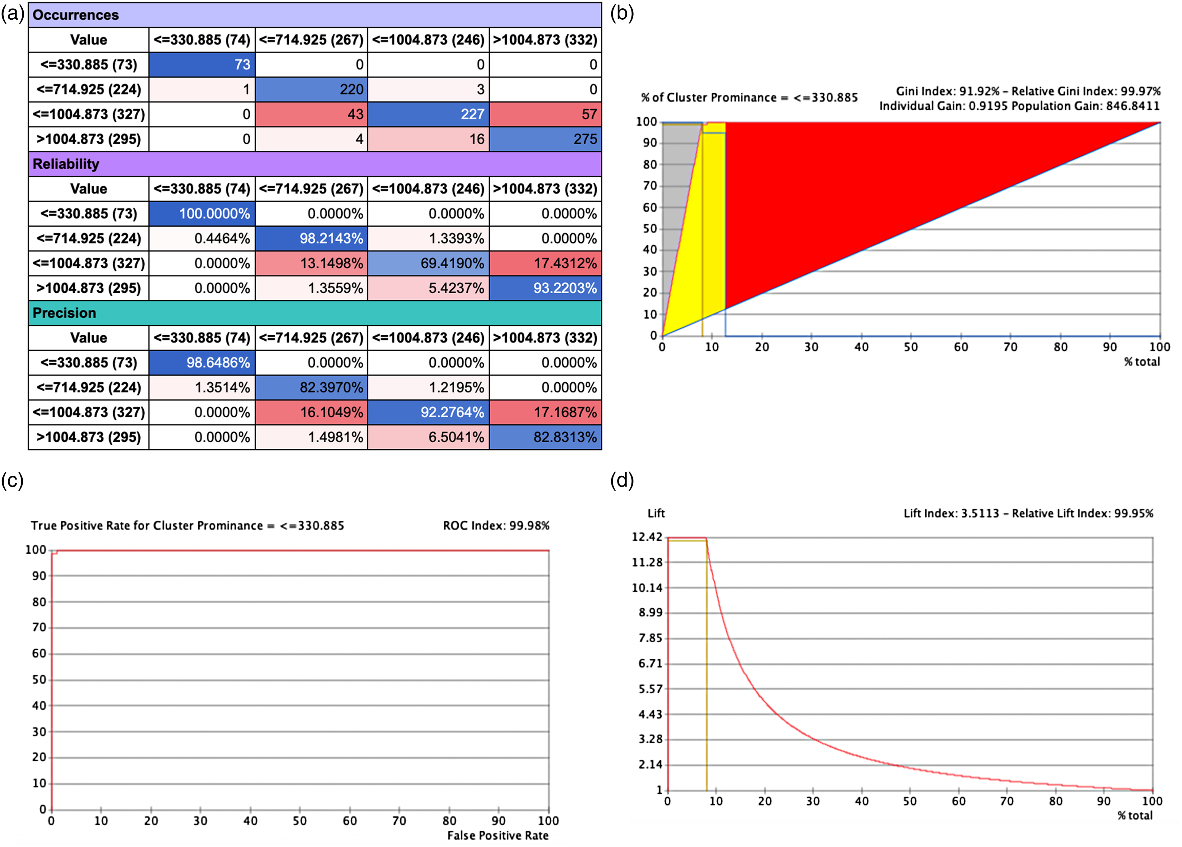
Network performance target evaluation Cluster Prominence node with other selected nodes (a) Occurrence, reliability and precision report; (b) Gain report of state ≤330.887, (c) ROC index of state ≤330.887, and (d) Lift index of state ≤330.887.

Figure 8 reflects the Tornado diagram of posterior probabilities to compute the significance of Cluster Prominence node with all nodes at different selected states. Table 3 shows the local analysis of the target state Cluster Prominence with state ≤330.887. The highest association was achieved with node Cluster shade with binary MI (0.19710), relative BMI (54.24%), binary relative significance (1.00), posterior mean value (1.540), and max Bayes factor (state ≤25.48 (1/4) with occurrence 93.93% and contribution of 7.33) followed by contrast with binary MI (0.1146), relative BMI (31.54%), binary relative significance (0.581), posterior mean (0.324), Max Bayes factor (state 0.397 (1/4) with occurrence 97.40% and contribution 5.11), and so on.

Figure 8.

Tornado diagram of posterior probabilities to compute the significance of Cluster Prominence node with all nodes at selected cluster states (≤330.887, ≤714.925, ≤1004.873, and > 1004.873).

Table 3.

Local analysis of target state cluster prominence with state ≤330.887.

Node	Binary MI	Relative BMI	Binary Relative sig.	Posterior mean value	Max Bayes Factor
Cluster shade	0.1971	54.24%	1.000	1.540	≤25.48 (1/4)	93.93%	7.33
Contrast	0.1146	31.54%	0.581	0.324	≤0.397 (1/4)	79.40%	5.11
Energy	0.0563	15.48%	0.286	0.334	≤0.462 (2/4)	79.35%	2.14
Correlation2	0.0359	9.88%	0.182	0.914	≤0.943 (3/4)	45.25%	1.69
Correlation	0.0359	9.88%	0.182	0.914	≤0.943 (3/4)	45.42%	1.69
AutoCorrelation	0.0330	9.08%	0.167	6.692	≤9.039 (1/4)	93.59%	1.57
Entropy	0.0259	7.13%	0.132	1.587	≤1.599 (2/4)	63.54%	1.83
Homogenity1	0.0023	0.63%	0.012	0.914	>0.925 (4/4)	46.66%	1.21
Dissimilarity	0.0012	0.34%	0.006	0.226	≤0.188 (1/4)	31.91%	1.19

Figure 9 reflects the structural coefficient analysis to reflect the strength of the association of arc frequency and v-structure frequency among GLCM extracted features. The highest 100% arc frequency was yielded between nodes $(D i s s i m i l a r i t y \to c o n t r a s t), C l u s t e r p r o m i n a n c e \to C o n t r a s t), C l u s t e r p r o m i n a n c e \to c l u s t e r s h a d e)$ followed by $(e n e e r g y \to e n t r o p y), (C l u s t e r s h a d e \to e n t r o p y))$ with 70% of arc frequency and $(C o r r e l a t i o n 2 \to c l u s t e r p r o m i n a n c e), h o m o g e n i t y 1 \to d i s s i m i l a r i t y), (C l u s t e r p r o m i n a n c e \to d i s s i m i l a r i t y)$ with 60% of arc frequency. Similarly, the highest v-structure with v-structure frequency of 100% was yielded with nodes $(C l u s t e r p r o m i n a n c e \to c l u s t e r s h a d e \to a u t o c o r r e l a t i o n), f o l l o w e d b y (e n e r g y \to c l u s t e r p r o m i n a n c e \to c o r r e l a t i o n 2)$ with 80% v-structure frequency and $(e n e r g y \to e n t r o p y \to c l u s t e r s h a d e)$ with 70% of v-structure frequency.

Figure 9.

Structural coefficient analysis based on learning of taboo algorithm.

Discussions and conclusions

The process segment discusses the machine learning advantages, hypotheses, and conditions for the following machine algorithms: Naive Bayes, decision tree, KNN, Neural Network, Support Vector Machine, and Genetic Algorithm. CAD operations are dynamic schemes built in the range of lung cancer diagnosis to identify and classify several lesions. A conventional CAD system involves processing multiple images, performing different tasks, and then classifying these into tumors or benign lesions.⁵⁷ The CAD device is used specifically to detect lung cancer. This method addresses the issue of designing a computer-based system to obtain the highest features from the differentiated unusual region of the lung CT image. Those features could be utilized to specifically identify lung tumors from the CT as favorable or destructive. A recent study achieved a sensitivity of 80% for detecting nodules with malignant potential and resulted in 0.85 false positive readings per section. In short, computer-aided diagnosis of lung nodules is likely to have an important role in CT-based screening tests in the near future.⁵⁸ The present research is consistent with similar studies investigated by utilizing BayesiaLab to determine the strength of relationship, causality among the features, node force, dynamic profile analysis, sensitivity analysis to further unfold the nonlinear hidden dynamics to further improve the diagnostic and prognostic such as brain tumor MRIs,¹² congestive heart failure,¹³ prostate cancer,⁵⁹ and lungs infection due to particulate matters.¹⁵ The results reveal that the proposed approach can be better utilized for early decision-making and improving the better diagnostic and prognostic system for patients suffering from lung pathologies.

The extraction of the most relevant features is a tedious task that requires specialist knowledge to compute the most relevant feature based on the choice of the problem. Previously, the researchers computed features based on texture, morphological, scale-invariant Feature transform, elliptic Fourier descriptors, and entropy features to detect the different pathologies in breast cancer and lung cancer. However, the extensions in texture features based on GLCM are further strengthening to improve lung cancer prediction which is proposed in this study. The GLCM features are widely used in medical image analysis, including lung cancer detection and diagnosis. GLCM features are extracted from the co-occurrence matrix that describes the distribution of gray-level pairs in an image. The GLCM features capture texture information and provide quantitative measures of the image's texture properties. Contrast measures the difference in intensity between neighboring pixels and is useful in distinguishing between regions with varying intensity levels. Correlation measures the linear relationship between pixel intensities and is useful in identifying patterns in the image. Energy measures the uniformity of gray-level values and is useful in identifying areas with homogeneous texture. Homogeneity measures the similarity between neighboring pixels and is useful in identifying areas with consistent texture. Entropy measures the randomness of gray-level values and is useful in identifying areas with complex texture.

In terms of ranking, if the goal is to identify differences between groups or features based on means, a t-test may be more appropriate. However, if the goal is to identify complex patterns and features based on their randomness or entropy, an entropy test may be more appropriate. In other cases, entropy-based methods may be more appropriate, such as when the data are nonparametric, or the goal is to identify informative features regardless of their relationship to the target variable.

To use BayesiaLab for lung cancer detection based on GLCM features, we constructed a BN. A BN is a graphical representation of the probabilistic relationships between variables. In this case, the variables computed were GLCM features and the presence or absence of lung cancer. The first step in building a BN is to define the variables and their relationships. We defined the GLCM features as the input variables and ranked these features based on t-test. We then kept the high-ranked features Cluster Prominence as our target variable. We then defined the conditional probabilities between these variables based on prior knowledge and available data. Once the BN was constructed, we used to make predictions about the presence or absence of lung cancer based on the GLCM features. To do this, we input the GLCM features into the network and calculated the probability of lung cancer given those features. A detailed analysis was then performed with the target variable such as exploratory analysis, relationship analysis, target optimization, segment profile analysis, network temporization analysis, dynamic profile analysis, and structural coefficient analysis. This approach can be more helpful to unfold the complete picture of the extracted nodes and their strengths and associations can help us to further investigate to build a better diagnostic system. The proposed approach will be very helpful to investigate the hidden complex and nonlinear dynamics and associations among the extracted GLCM features which can be further utilized to improve the prognosis and diagnosis of lung cancer and can assist healthcare practitioners to provide better disease decision-making system. The proposed approach will further help to decrease the mortality rate.

There are few limitations of the study, as currently, the dataset is single centric study and lacks of clinical information of the patients, thus need more computational methods with hyperparameters optimization to manage the multicenter studies. In the future, the proposed approach can be utilized on depository dataset from different facility to authenticate the results for larger and multicentric study. Multicentric studies have several advantages over single-center study and are commonly used in medical research, where they may involve several hospitals, clinics, or research centers collaborating on a common research question.

For example, a multicentric study might investigate the effectiveness of a new cancer treatment by collecting data from patients treated at different hospitals across the country or the world. The advantages of multicentric studies include the ability to recruit a large and diverse sample, which can increase the generalizability of the results, and the ability to combine resources and expertise from multiple sites. We will apply the proposed methods on a larger dataset with more clinical information of the patients.

Footnotes

Acknowledgments

This work was supported by the King Khalid University, Abha, Saudi Arabia. The authors extend their appreciation to the Deanship of Scientific Research at King Khalid University for funding this work through Larg Groups Project under grant number (R.G.P. 2/43/44). Princess Nourah bint Abdulrahman University Researchers Supporting Project number (PNURSP2023R192), Princess Nourah bint Abdulrahman University, Riyadh, Saudi Arabia. The authors would like to thank the Deanship of Scientific Research at Shaqra University for supporting. This study is supported via funding from Prince Sattam Bin Abdulaziz University project number PSAU/2023/R/1444

Contributorship: JY, PLY, AAK, HK, MSK, and AO edited the paper. AA conceptualized the study and edit the paper. AEJ AA conceptualized the study and edit the paper. LH conceptualized the study, analyzed data, and wrote the paper.

Consent statement

A publicly available dataset from was taken which is detailed and recently used in Hussain et al,²⁹ so the patient consent is not necessary.

Declaration of conflicting interests

The author(s) declares that they do not have any conflict of interest.

Ethical approval

A publicly available dataset from was taken which is detailed and recently used in Hussain et al.²⁹

Funding

The author(s) received no financial support for the research, authorship, and/or publication of this article.

Guarantor

N/A

ORCID iD

Lal Hussain

References

Siegel

Miller

Jemal

. Cancer statistics, 2018. CA Cancer J Clin 2018; 68: 7–30.

Oser

Niederst

Sequist

, et al. Transformation from non-small-cell lung cancer to small-cell lung cancer: molecular drivers and cells of origin. Lancet Oncol [Internet] 2015; 16: e165–e172. https://linkinghub.elsevier.com/retrieve/pii/S1470204514711805 .

Krishnaiah

Narsimha

Subhash

, et al. Diagnosis of lung cancer prediction system using data mining classification techniques. Int J Comput Sci Inf Technol 2013; 4: 39–45.

Manikandan

Bharathi

. Lung cancer detection using fuzzy auto-seed cluster means morphological segmentation and SVM classifier. J Med Syst [Internet] 2016; 40: 181. http://link.springer.com/10.1007/s10916-016-0539-9 .

Rubio

JdJ

Cruz

Elias

, et al. ANFIS system for classification of brain signals. J Intell Fuzzy Syst [Internet] 2019; 37: 4033–4041. https://www.medra.org/servlet/aliasResolver?alias=iospress&doi=10.3233/JIFS-190207 .

Nithila

Kumar

. Segmentation of lung nodule in CT data using active contour model and fuzzy C-mean clustering. Alex Eng J [Internet] 2016; 55: 2583–2588. https://linkinghub.elsevier.com/retrieve/pii/S1110016816301399 .

Kaikkonen

Parviainen

Rahikainen

, et al. Bayesian networks in environmental risk assessment: a review. Integr Environ Assess Manag [Internet] 2021; 17: 62–78. https://onlinelibrary.wiley.com/doi/10.1002/ieam.4332 .

Kocian

Massa

Cannazzaro

, et al. Dynamic Bayesian network for crop growth prediction in greenhouses. Comput Electron Agric [Internet] 2020; 169: 105167. https://linkinghub.elsevier.com/retrieve/pii/S0168169919321131 .

Amaral

Oliveira

Eghrari

, et al. Bayesian network: a simplified approach for environmental similarity studies on maize. Crop Breed Appl Biotechnol [Internet] 2019; 19: 70–76. http://www.scielo.br/scielo.php?script=sci_arttext&pid=S1984-70332019000100070&tlng=en .

10.

Laurila-Pant

Mäntyniemi

Venesjärvi

, et al. Incorporating stakeholders’ values into environmental decision support: a Bayesian belief network approach. Sci Total Environ [Internet] 2019; 697: 134026. https://linkinghub.elsevier.com/retrieve/pii/S0048969719340033 .

11.

Zhang

Pan

Wang

, et al. Bayesian network construction and genotype-phenotype inference using GWAS statistics. IEEE/ACM Trans Comput Biol Bioinform [Internet] 2019; 16: 475–489. https://ieeexplore.ieee.org/document/8126853/ .

12.

Hussain

Malibari

Alzahrani

, et al. Bayesian dynamic profiling and optimization of important ranked energy from gray level co-occurrence (GLCM) features for empirical analysis of brain MRI. Sci Rep [Internet] 2022; 12: 15389. https://www.nature.com/articles/s41598-022-19563-0 .

13.

Eltahir

Hussain

Malibari

, et al. A Bayesian dynamic inference approach based on extracted gray level co-occurrence (GLCM) features for the dynamical analysis of congestive heart failure. Appl Sci [Internet] 2022; 12: 6350. https://www.mdpi.com/2076-3417/12/13/6350 .

14.

Kim

Park

Jeon

, et al. Usage dynamics of environmental sustainability indicators for manufacturing and service systems. J Clean Prod [Internet] 2022; 360: 132062. https://linkinghub.elsevier.com/retrieve/pii/S0959652622016699 .

15.

Albraikan

Alzahrani

Negm

, et al. Future challenges of particulate matters (PMs) monitoring by computing associations among extracted multimodal features applying Bayesian network approach. Appl Artif Intell [Internet] 2022: 36. https://www.tandfonline.com/doi/full/10.1080/08839514.2022.2112545 .

16.

Mulhern

Roostaei

Schwetschenau

, et al. A new approach to a legacy concern: evaluating machine-learned Bayesian networks to predict childhood lead exposure risk from community water systems. Environ Res [Internet] 2022; 204: 112146. https://linkinghub.elsevier.com/retrieve/pii/S001393512101447X .

17.

Zhang

Cai

, et al. A Bayesian network prediction model for microvascular invasion in patients with intrahepatic cholangiocarcinoma: a multi-institutional study. World J Surg [Internet] 2023; 47: 773–784. https://link.springer.com/10.1007/s00268-022-06867-5 .

18.

Khan

Yin

Mustafa

, et al. Analyzing human factor involvement in sustainable hazardous cargo port operations. Ocean Eng [Internet] 2022; 250: 111028. https://linkinghub.elsevier.com/retrieve/pii/S0029801822004486 .

19.

Zhang

Cai

, et al. A Bayesian network prediction model for gallbladder polyps with malignant potential based on preoperative ultrasound. Surg Endosc [Internet] 2023; 37: 518–527. https://link.springer.com/10.1007/s00464-022-09532-z .

20.

Amzil

Yahia

Klement

, et al. Automatic neural networks construction and causality ranking for faster and more consistent decision making. Int J Comput Integr Manuf [Internet] 2022; 36: 1–21.

21.

De Giovanni

Belvedere

Grando

. The selection of industry 4.0 technologies through Bayesian networks: an operational perspective. IEEE Trans Eng Manag [Internet] 2022; 70: 1–16. https://ieeexplore.ieee.org/document/9889097/ .

22.

de Waal

Joubert

. Explainable Bayesian networks applied to transport vulnerability. Expert Syst Appl [Internet] 2022; 209: 118348. https://linkinghub.elsevier.com/retrieve/pii/S0957417422014671 .

23.

Sperotto

Molina

Torresan

, et al. A Bayesian networks approach for the assessment of climate change impacts on nutrients loading. Environ Sci Policy [Internet] 2019; 100: 21–36. https://linkinghub.elsevier.com/retrieve/pii/S1462901118311705 .

24.

Gandhi

Armstrong

Petkar

. PredictingRice crop yield using Bayesian networks. 2016 Int Conf Adv Comput Commun Informatics [Internet]. IEEE; 2016. p. 795–799. http://ieeexplore.ieee.org/document/7732143/.

25.

Corrales

. Toward detecting crop diseases and pest by supervised learning. Ing Univ [Internet] 2015; 19: 207. http://revistas.javeriana.edu.co/index.php/iyu/article/view/6732 .

26.

Musango

Peter

. A Bayesian approach towards facilitating climate change adaptation research on the South African agricultural sector. Agrekon [Internet] 2007; 46: 245–259. http://www.tandfonline.com/doi/abs/10.1080/03031853.2007.9523770 .

27.

Ershadi

Seifi

. An efficient Bayesian network for differential diagnosis using experts’ knowledge. Int J Intell Comput Cybern [Internet] 2020; 13: 103–126. https://www.emerald.com/insight/content/doi/10.1108/IJICC-10-2019-0112/full/html .

28.

Newlands

Carisse

, et al. Disease risk forecasting with Bayesian learning networks: application to grape powdery mildew (Erysiphe necator) in vineyards. Agronomy [Internet] 2020; 10: 622. https://www.mdpi.com/2073-4395/10/5/622 .

29.

Hussain

Aziz

Alshdadi

AAA

, et al. Analyzing the dynamics of lung cancer imaging data using refined fuzzy entropy methods by extracting different features. IEEE Access [Internet] 2019; 7: 64704–64721. https://ieeexplore.ieee.org/document/8716659/ .

30.

Hussain

Aziz

Saeed

, et al. Arrhythmia detection by extracting hybrid features based on refined fuzzy entropy (FuzEn) approach and employing machine learning techniques. Waves Random Complex Media 2020; 30:656–686.

31.

Hussain

Saeed

Awan

, et al. Detecting brain tumor using machine learning techniques based on different features extracting strategies. Curr Med Imaging Former Curr Med Imaging Rev [Internet] 2019; 15: 595–606. http://www.eurekaselect.com/163868/article .

32.

Hussain

. Detecting epileptic seizure with different feature extracting strategies using robust machine learning classification techniques by applying advance parameter optimization approach. Cogn Neurodyn [Internet] 2018; 12: 271–294. http://link.springer.com/10.1007/s11571-018-9477-1 .

33.

Hussain

Aziz

Khan

, et al. Machine learning based congestive heart failure detection using feature importance ranking of multimodal features. Math Biosci Eng [Internet] 2021; 18: 69–91. http://aimspress.com/article/doi/10.3934/mbe.2021004 .

34.

Hussain

Ahmed

Saeed

, et al. Prostate cancer detection using machine learning techniques by employing combination of features extracting strategies. Cancer Biomarkers [Internet] 2018; 21: 393–413. http://www.medra.org/servlet/aliasResolver?alias=iospress&doi=10.3233/CBM-170643 .

35.

Haralick

Shanmugam

. 04309314. 1973.

36.

Olaniyi

Adekunle

Odekuoye

, et al. Automatic system for grading banana using GLCM texture feature extraction and neural network arbitrations. J Food Process Eng [Internet] 2017; 40: e12575.

37.

Campbell

Kang

Shokouhi

. Application of Haralick texture features in brain [18F]-florbetapir positron emission tomography without reference region normalization. Clin Interv Aging [Internet] 2017; 12: 2077–2086. https://www.dovepress.com/application-of-haralick-texture-features-in-brain-18f-florbetapir-posi-peer-reviewed-article-CIA .

38.

Shahajad

Gambhir

Gandhi

. Features extraction for classification of brain tumor MRI images using support vector machine. 2021 11th Int Conf Cloud Comput Data Sci Eng [Internet]. IEEE; 2021. p. 767–772. https://ieeexplore.ieee.org/document/9377111/.

39.

James

Heddallikar

Choudhari

, et al. Analysis of Features in SAR Imagery Using GLCM Segmentation Algorithm. 2021. p. 253–266. https://link.springer.com/10.1007/978-981-16-1681-5_16.

40.

Wang

Khoshgoftaar

Gao

. A comparative study of filter-based feature ranking techniques. 2010 IEEE Int Conf Inf Reuse Integr [Internet]. IEEE; 2010. p. 43–48. http://ieeexplore.ieee.org/document/5558966/.

41.

Zhang

Liang

, et al. A Matlab Toolbox for Feature Importance Ranking. 2019 Int Conf Med Imaging Phys Eng [Internet]. IEEE; 2019. p. 1–6. https://ieeexplore.ieee.org/document/9098233/.

42.

Kim

. T test as a parametric statistic. Korean J Anesthesiol [Internet] 2015; 68: 540. http://ekja.org/journal/view.php?doi=10.4097/kjae.2015.68.6.540 .

43.

Pearl

. Fusion, propagation, and structuring in belief networks. Artif Intell 1986; 29: 241–288.

44.

Bayesia

. BayesiaLab7. Bayesia USA 305 Lockhart Court Franklin, TN 37069 USA. 2017.

45.

Shannon

. A mathematical theory of communication. Bell Syst Tech J 1948; 27: 379–423.

46.

Xiao

Gao

, et al. Inferring gene regulatory networks using conditional regulation pattern to guide candidate genes. PLoS One 2016; 11: 1–13.

47.

Janzing

Balduzzi

Grosse-Wentrup

, et al. Quantifying causal influences. Ann Stat 2013; 41: 2324–2358.

48.

Conrady

Jouffe

. Bayesian networks and BayesiaLab: A practical introduction for researchers. New York: Bayesia USA, 2015.

49.

Harris

Bhuvaneshwar

Natarajan

, et al. Pharmacogenomic characterization of gemcitabine response – a framework for data integration to enable personalized medicine. Pharmacogenet Genomics [Internet] 2014; 24: 81–93. https://journals.lww.com/01213011-201402000-00001 .

50.

Thai

Campo

Lara

, et al. Convergence and coevolution of Hepatitis B virus drug resistance. Nat Commun [Internet] 2012; 3: 789. http://www.nature.com/articles/ncomms1794 .

51.

Moreno-Jiménez

García-Gómez

Oropesa

, et al. Screening risk assessment tools for assessing the environmental impact in an abandoned pyritic mine in Spain. Sci Total Environ [Internet] 2011; 409: 692–703. https://linkinghub.elsevier.com/retrieve/pii/S0048969710011745 .

52.

Wilhere

. Using Bayesian networks to incorporate uncertainty in habitat suitability index models. J Wildl Manage [Internet] 2012; 76: 1298–1309. https://onlinelibrary.wiley.com/doi/10.1002/jwmg.366 .

53.

Tanackov

Janković

Sremac

, et al. Risk distribution of dangerous goods in logistics subsystems. J Loss Prev Process Ind [Internet] 2018; 54: 373–383. https://linkinghub.elsevier.com/retrieve/pii/S0950423016305071 .

54.

Goerlandt

Montewka

. Maritime transportation risk analysis: review and analysis in light of some foundational issues. Reliab Eng Syst Saf [Internet] 2015; 138: 115–134. https://linkinghub.elsevier.com/retrieve/pii/S0951832015000356 .

55.

Hänninen

Kujala

. Influences of variables on ship collision probability in a Bayesian belief network model. Reliab Eng Syst Saf [Internet] 2012; 102: 27–40. https://linkinghub.elsevier.com/retrieve/pii/S0951832012000245 .

56.

Kruschke

. Bayesian Estimation supersedes the t test. J Exp Psychol Gen [Internet] 2013; 142: 573–603.

57.

Yu-Jen Chen

Y-J

Hua

K-L

Hsu

C-H

, et al. Computer-aided classification of lung nodules on computed tomography images via deep learning technique. Onco Targets Ther [Internet] 2015; 2015–2022. http://www.dovepress.com/computer-aided-classification-of-lung-nodules-on-computed-tomography-i-peer-reviewed-article-OTT.

58.

Armato

Roy

MacMahon

, et al. Evaluation of automated lung nodule detection on low-dose computed tomography scans from a lung cancer screening program1. Acad Radiol 2005; 12: 337–346.

59.

Hussain

Ali

Rathore

, et al. Applying Bayesian network approach to determine the association between morphological features extracted from prostate cancer images. IEEE Access [Internet] 2019; 7: 1586–1601. https://ieeexplore.ieee.org/document/8579592/ .

Intelligent lung cancer MRI prediction analysis based on cluster prominence and posterior probabilities utilizing intelligent Bayesian methods on extracted gray-level co-occurrence (GLCM) features

Abstract

Keywords

Introduction

Materials and methods

Dataset

Feature extraction

Feature importance ranking algorithms

T-test method for feature ranking

Bayesian network analysis

Statistical analysis

Exploratory analysis of the unsupervised network

Sensitivity analysis

Segment profile analysis of energy

Results

Discussions and conclusions

Footnotes

Acknowledgments

Consent statement

Declaration of conflicting interests

Ethical approval

Funding

Guarantor

ORCID iD

References