Sage Journals: Discover world-class research

Abstract

The abnormal growth of human healthy cells is called cancer. One of the major types of cancer is sarcoma, mostly found in human bones and soft tissue cells. It commonly occurs in children. According to a survey of the United States of America, there are more than 17,000 sarcoma patients registered each year which is 15% of all cancer cases. Recognition of cancer at its early stage saves many lives. The proposed study developed a framework for the early detection of human sarcoma cancer using deep learning Recurrent Neural Network (RNN) algorithms. The DNA of a human cell is made up of 25,000 to 30,000 genes. Each gene is represented by sequences of nucleotides. The nucleotides in a sequence of a driver gene can change which is termed as mutations. Some mutations can cause cancer. There are seven types of a gene whose mutation causes sarcoma cancer. The study uses the dataset which has been taken from more than 134 samples and includes 141 mutations in 8 driver genes. On these gene sequences RNN algorithms Long and Short-Term Memory (LSTM), Gated Recurrent Units and Bi-directional LSTM (Bi-LSTM) are used for training. Rigorous testing techniques such as Self-consistency testing, independent set testing, 10-fold cross-validation test are applied for the validation of results. These validation techniques yield several metrics such as Area Under the Curve (AUC), sensitivity, specificity, Mathew's correlation coefficient, loss, and accuracy. The proposed algorithm exhibits an accuracy of 99.6% with an AUC value of 1.00.

Keywords

Long and short-term memory (LSTM) network gated recurrent units and bi-directional LSTM sarcoma cancer self-consistency test independent set test 10-fold cross-validation test receiver operating characteristic (ROC) curve

Introduction

Genomics in molecular biology is the study of the structure and function of genomes. Every human cell is made up of 25,000 to 30,000 genes. Every gene carries specific information for the proper functioning of the cell. It also carries the information that is passed from the parents to the offspring.^1,2 Every genome is made up of a special sequence of genes. For the complete study of the genome, it is necessary to understand the structure of genes in it. A single gene does not provide a global perspective of all aspects of a cell, so it is necessary to understand the sequence of genes connected.^3,4 Every genome has four bases (Adenine “A,” Thymine “T,” Guanine “G,” Cytosine “C”). The change in the sequence of the base of DNA causes mutation⁵ and mutation is one of the most common causes of genetic disorders. Cancer is also caused by mutation.^6,7

Four types of mutation in genes include base substitution, insertion, deletion, and inversion,⁵ as shown in Figure 1. “T,” “C,” and “A” are replaced with “G,” “T,” and “G” in Figure 1 and known as base substitution. In Figure 1, base “A” is added to the sequence that is called insertion. In Figure 1, base “C” is deleted from the sequence, that is called a deletion. The segment “ACT” is reversed as “TCA” in Figure 1 which is known as inversion.

Fig. 1.

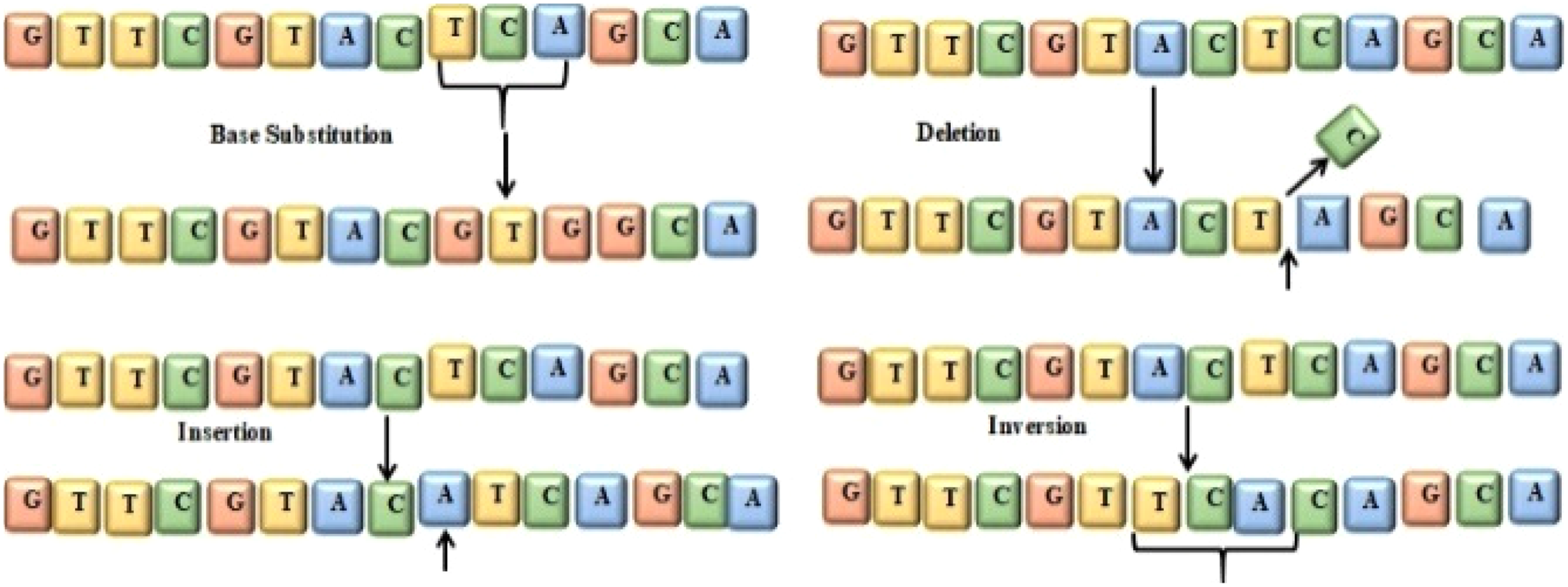
Mutation in gene base.

Genetic mutation can disturb the functional characteristics of a gene that may cause cancer. Such disturbance creates an unbalance between the growth of cells (Mitosis) and the destruction of cells (apoptosis) that leads to the development or progression of cancer. Tools and methodologies that help to identify mutations that cause cancer at an early stage are a dire need. Cancer can be successfully treated if the patient is diagnosed at an early stage of cancer.

Different types of cancer exist in humans. Sarcoma is the unhealthy growth of human bone and soft tissue cells. 60% of sarcoma cancer cases occur in arms and legs. It is a childhood cancer and rarely occurs in adults. Sarcoma is rare in adults making up about 1% of all adult cancers. However, it occurs more abundantly in children comprising about 15% of all childhood cancers.⁸ In the United States of America about 17,000 sarcoma cases are registered each year. There are different types of sarcoma cancers such as deep skin tissue sarcoma, Osteosarcoma, blood vessels sarcoma, Kaposi's sarcoma, angiosarcoma, bone cancer, chordoma, chondrosarcoma, desmoid-type fibromatosis, and Ewing sarcoma, etc. One of the best techniques for the detection of sarcoma is to detect circulating tumor cells from marginal blood vessels.³ Biopsy is the main technique used for the detection of soft tissue sarcoma. This technique works by examining a small tissue cell under a microscope. Core Needle Biopsy and Surgical Biopsy are used for the detection of tissue sarcoma from an obtained tissue sample.

Artificial intelligence (AI) is gaining popularity in the field of medical science. AI is used in medical science for the detection of various diseases.

This study uses AI-based techniques for the early detection of sarcoma. Recurrent Neural Networks (RNNs) and Convolutional Neural Networks (CNNs) are the most popular deep learning (DL) models. CNN has inherently evolved as a classifier for images or two-dimensional data while RNN is more suited for text classification.^9,10 The dataset used in this work contains gene sequences which are essentially text-based data and henceforth recurrent networks are proposed.

Literature review

In this section, some computational studies for the detection and identification of sarcoma cancer are discussed. Soft tissue sarcoma (STS) is a type of sarcoma cancer that is present in the tissues that connect and support the body. In a study regarding the identification of STS 20 attributes were identified, out of which 15 are numeric and five are of categoric nature. This dataset was assembled from 50 participants of age between 1 and 77 years. Machine learning algorithms like Support vector machines and Decision trees are used for the classification of the dataset.^11–13

Radiomics-based machine learning algorithm is also used for the detection of metastases from STS. A dataset consisting of 54 training sets and 23 validation test sets is used for this study. Three methods RelieEf, LASSO, and UDFS are used for feature extraction.¹⁴

Fuzzy Clustering and Neuro-fuzzy classifier is also used for the detection of bone sarcoma. 120 patients’ data is used for this study for the detection of bone sarcoma. An adaptive neuro-fuzzy inference system (ANFIS) is used for the classification of benign and malignant bone cancer. MR images of bones are used for extracting gray-level co-occurrence matrix features.¹⁵ The accuracy of this model is 93.75%.

In another study, the author used five cohorts of data set. They used the combination of Digital pathology and Deep learning for the detection of sarcoma cancer. A deep Convolutional neural network is designed for the data set for a batch of 32. In every cohort, cross-validation is applied. The DL method achieved a mean AUROC of 0.97 for diagnosing the five most common STS subtypes.¹⁶ The most common type of children’s sarcoma is Ewing sarcoma. An immune-related gene signature based on machine learning is identified for the detection of Ewing Sarcoma (ES). A total of 249 database and extracted differential expressed immune-related genes were screened for this method from which 11-gene signature were the strongest correlation where patient prognoses were analyzed using a machine learning algorithm. The 11-gene signature also had a high prognostic value in the ES external verification in ES.¹⁷ The accuracy of this model is 87%. This study is also using machine learning techniques for the detection of mutation in sarcoma.

Eight supervised machine learning methods were used for tissue classification of multi-parametric MRI measurements in soft-tissue sarcomas. Data from 18 sarcoma patients are used for this research. LR, SVM, RF, KNN, Kernel Density Estimation, NB, and Neural network with 20 nodes are used for classification using the Scikit-Learn software package.¹⁸ The high median cross-validation accuracies of these methods are between 80% and 85%. Naïve Bayes (NB) gives relatively short training and prediction times of 0.73 and 0.69 microsecond, respectively on a 3.5 GHz personal machine. The summary of the previous work is also written in Table 1.

Table 1.

Summary of the previous work.

Paper citation	Algorithms	Accuracy achieved
¹⁵	ANFIS	93.75%
¹⁶	Densely Connected Convolutional Network	97%
¹⁷	Regression Analysis	87%
¹⁹	Naive Bayesian, Decision Tree, Support Vector Machine and Random Forest	72.5%
²⁰	Markov model with feature hashing	82.83%
²¹	Support Vector Machine	93%
²²	RNN, LSTM, GRU	78%

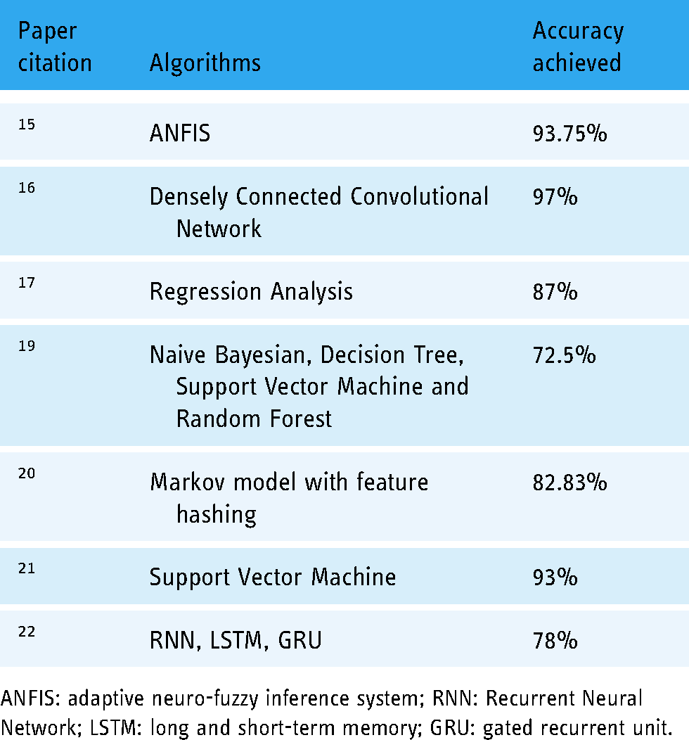
ANFIS: adaptive neuro-fuzzy inference system; RNN: Recurrent Neural Network; LSTM: long and short-term memory; GRU: gated recurrent unit.

Numerous limitations and constraints were observed in the current state-of-the-artwork. No generalized and explicit benchmark dataset for sarcoma-based mutations along with specific sequences has been compiled.²² Further, evaluation techniques are not sufficiently rigorous and convincing. Subsequently, there seems to be adequate room for improvement in the accuracy of the models. Keeping these limitations in view this study has compiled the latest and more generalized dataset as discussed in the data acquisition framework. Furthermore, multiple DL algorithms are exploited to achieve an overall accuracy of 99.6%. Multiple evaluations and validation techniques such as a self-consistency test, independent set test, and 10-fold cross-validation test are probed. The evaluation metrics sensitivity, specificity, Area under the curve, and Matthew's correlation coefficient are also estimated as discussed in Table 3.

Table 3.

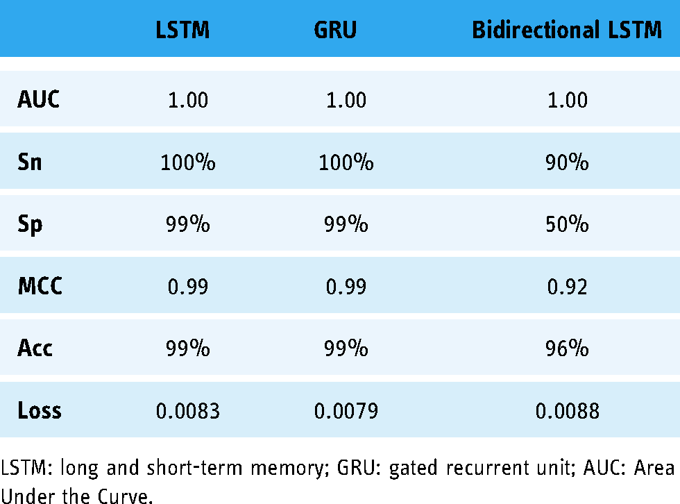
Results of self-consistency test.

	LSTM	GRU	Bidirectional LSTM
AUC	1.00	1.00	1.00
Sn	99%	99%	99%
Sp	100%	100%	100%
MCC	0.99	0.99	0.99
Acc	99%	99%	99%
Loss	0.0078	0.0081	0.0077

LSTM: long and short-term memory; GRU: gated recurrent unit; AUC: Area Under the Curve.

Materials and methods

In this section, a detailed description and usage of the feature extraction and classification processes in terms of their internal working is discussed. The study can be described via systematic phases which include Data Acquisition Framework, Feature Extraction Framework (FEF), training of classifiers using a cohort of DL models, testing and validation, and evaluation using well-defined metrics. The graphical representation of the flow of the proposed model is depicted in Figure 2.

Fig. 2.

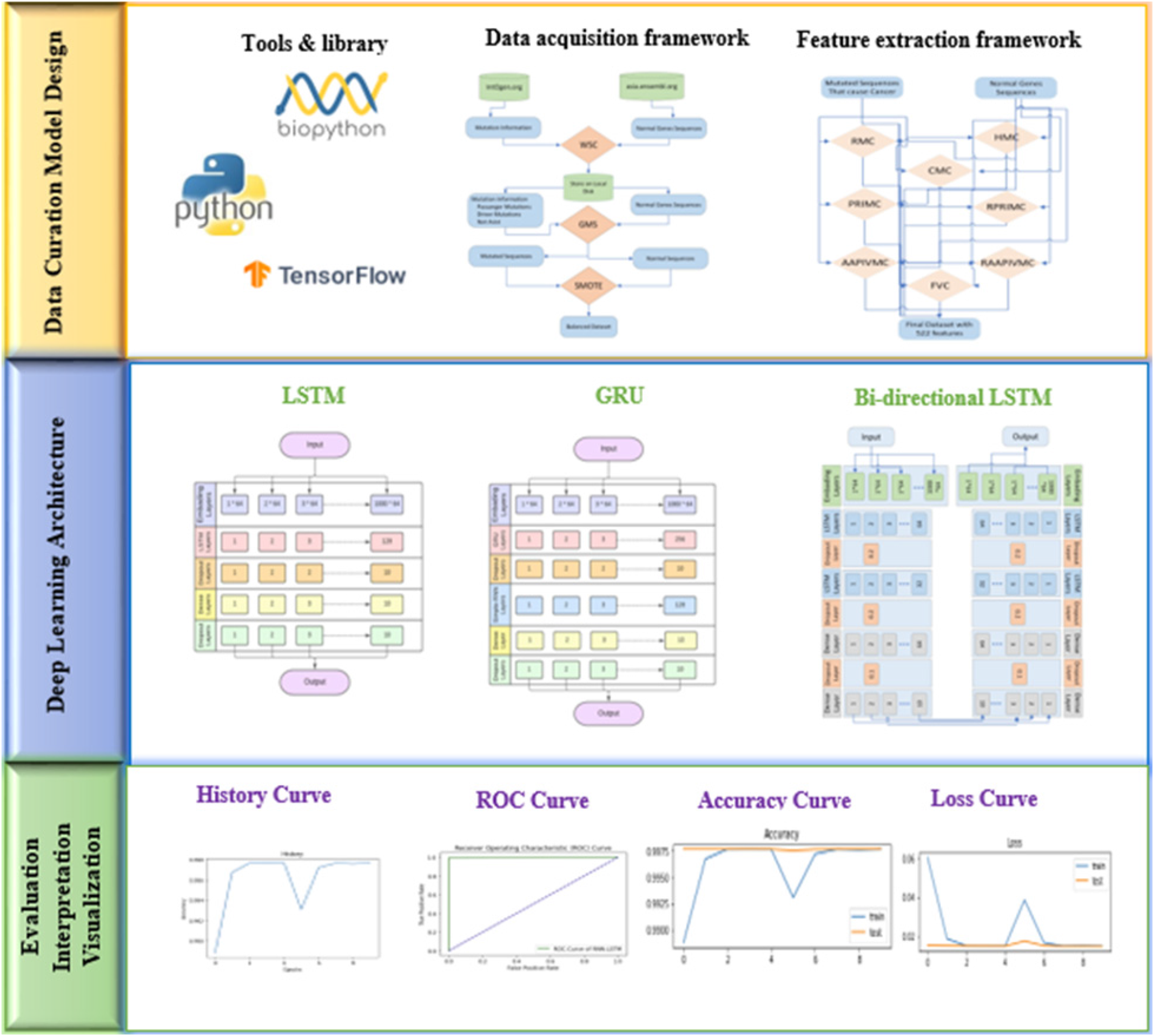
The graphical representation of the proposed model.

Data acquisition framework

A robust benchmark dataset is the key enabler of any classification problem. Typically, features and other relevant information is extracted from the benchmark dataset that helps in training and testing the proposed learning and predictive frameworks. Keeping in view the importance of the dataset in devising a proposed predictive framework, the method of benchmark dataset acquisition is discussed in a detailed manner. Dataset is comprised such that it consists of Normal sequences as well as mutated sequences. Normal sequences are extracted from asia.ensembl.org²³ through web scrapping code (WSC) while mutated sequence cannot be extracted through web scrapping directly from any source. Although mutation information is available at intOGen.Org.²⁴ This mutation information is extracted using WSC. The data acquisition framework is also explained with the help of a diagram in Figure 3.

Fig. 3.

Benchmark dataset generation process.

Generate Mutated Sequences code is also provided to transform the normal sequences into mutated sequences based on available mutation information and subsequently label it as a passenger, not assist or driver mutation. Where driver mutation is the class of interest that causes cancer.²⁵

Dataset used in this study consists of 134 human samples and 141 mutations. Whereas eight types of diverse genes along with their mutation information are collected from the said human samples and are listed in Table 2.

Table 2.

Genes involved in sarcoma cancer and number of mutations.

Gene Symbol	Mutations	Samples
TP53	75	65
ATRX	23	31
RB1	18	14
PIK3CA	6	7
NF1	4	5
PTEN	6	5
TET2	6	4
RET	3	3

The genes listed in Table 2 have been identified to cause sarcoma cancer in humans as revealed in numerous studies.²⁶ The dataset consists of 134 samples, eight genes, and 141 mutations. The word cloud of the mutated sequences is represented in Figure 4.

Fig. 4.

World cloud of related gene sequences.

It is necessary that any bias from the unbalanced dataset in the training and testing of the proposed predictive framework is addressed preemptively. Sampling and Oversampling are used to balance the available dataset. In the under-sampling technique, the number of samples of the majority classes are reduced to balance the dataset. While oversampling techniques increase the number of samples in minority classes.²⁷

The dataset is denoted by D, which is defined in equation (1)

D = D^{+} U D^{-}

(1)

Here

D^{+}

is considered as a mutated sequence that causes cancer while

D^{-}

is considered as Normal sequences and passenger mutations that do not cause cancer and U is the union for both sequences.

Feature extraction framework

The learning algorithms consume input in quantitative form. The proposed model incorporates numerous basic quantitative encodings and dimensionality reduction techniques using various feature extraction techniques. An FEF is developed to extract useful features from the given dataset for training and testing purposes. FEF will help the DL models to increase learning accuracy.^28,29 The operational workflow of FEF is presented in Figure 5. It consists of information-oriented statistical operations to quantify different types of information contained inside the DNA Sequences.

Fig. 5.

Feature extraction framework.

Statistical moments

The statistical characterization of data is helpful to estimate the general behavior of its randomness. That's why in this work, statistical moments are applied to transform genomic data into required fixed size. Every chosen statistical moment identifies certain information to represent the nature of data. Hahn moment (HM), central moment (CM), and raw moment (RM) of the genomic data provide the valuable components of the input vector to be utilized by the predictor. HM requires two-dimensional data in the form of a square matrix; therefore, the genomic sequences are converted into a two-dimensional notation 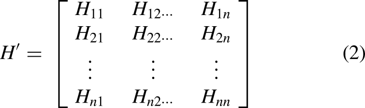$H^{'}$ of size $x * x$ as given in equation (2).

H^{'} = [\begin{matrix} H_{11} & H_{12 \dots} & H_{1 n} \\ H_{21} & H_{22 \dots} & H_{2 n} \\ \begin{matrix} ⋮ \\ H_{n 1} \end{matrix} & \begin{matrix} ⋮ \\ H_{n 2 \dots} \end{matrix} & \begin{matrix} ⋮ \\ H_{n n} \end{matrix} \end{matrix}]

(2)

Here H defines the gene sequence.³⁰

The advantage of the obtained matrix is twofold. It is exploited to compute the statistical moments for dimensionality reduction and having fixed-sized feature vectors.

HMs are reversible and present the symmetrical nature of data. That reversibility means that original data can be constructed using the HMs. The computed HM is exploited by the predictor through the corresponding feature vector. HM is calculated by using the following Hahn polynomial

\begin{aligned} h_{n}^{r, s} (P, Q) & = (Q + V - 1)_{n} (Q - 1)_{n} \\ \times \sum_{z = 0}^{n} (- 1)^{z} \frac{{(- n)}_{z} {(- p)}_{z} {(2 Q + r + s - n - 1)}_{z}}{{(Q + s - 1)}_{z} {(Q - 1)}_{z}} \frac{1}{z!} \end{aligned}

(3)

H_{x y} = \sum_{j = 0}^{G - 1} \sum_{i = 0}^{G - 1} δ_{x y} h_{x}^{a, b} (j, Q) h_{y}^{a, b} (j, Q), m, n = 0, 1, 2, . . ., Q - 1

(4)

RM are place and scale variants. It is the most common type of statistical moment. It is used for means, asymmetry, and variance calculation of probability distribution. The RM is used for data imputation. Imputation is the process of replacing the missing data values in a dataset with the most substitute values to preserve the information.^31,32 The RMs of 2D data with order

r + s

is expressed by equation 5.

U_{r s} = \sum_{e = 1}^{n} \sum_{f = 1}^{n} e^{r} f^{s} δ_{e f}

(5)

Centroids

(r, s)

are required to compute the CMs that are visualized as the center of data. By exploiting the centroids, CMs can be computed as³⁰

V_{r s} = \sum_{e = 1}^{n} \sum_{f = 1}^{n} (e - \bar{x})^{r} (f - \bar{y})^{s} δ e f

(6)

Position relative incidence matrix

The position relative incidence matrix (PRIM) plays a key role in determining the relative positioning of nucleotide bases. The significance of the position where the said base is placed and the precise role of nucleotide bases regarding the mapping of gene attributes is critical. It is defined as two-dimensional matric, described in equation (7)

R_{P R I M} = [\begin{matrix} \begin{matrix} R_{1 \to 1} & R_{1 \to 2 \dots} \\ R_{2 \to 1} & R_{2 \to 2 \dots} \end{matrix} & \begin{matrix} R_{1 \to q \dots} \\ R_{2 \to q \dots} \end{matrix} & \begin{matrix} R_{1 \to M} \\ R_{2 \to M} \end{matrix} \\ \begin{matrix} ⋮ & ⋮ \\ R_{p \to 1} & R_{p \to 2 \dots} \end{matrix} & \begin{matrix} ⋮ \\ R_{p \to q \dots} \end{matrix} & \begin{matrix} ⋮ \\ R_{p \to M} \end{matrix} \\ \begin{matrix} ⋮ & ⋮ \\ R_{M \to 1} & R_{M \to 2 \dots} \end{matrix} & \begin{matrix} ⋮ \\ R_{M \to q \dots} \end{matrix} & \begin{matrix} ⋮ \\ R_{M \to M} \end{matrix} \end{matrix}]

(7)

Here

R_{p \to q}

represents the cluster of relative places of qth base with respect to the first occurrence of the pth base. The matrix can then be exploited to compute HM, CM and RMs.

Reverse position relative incidence matrix

Diversity always provides the reliability of the features obtained using certain statistical techniques by rearranging and reshuffling the gene sequences. The reverse position relative incidence matrix (RPRIM) is calculated by reversing the original gene sequences as described in equation (8).²⁸ Like PRIM, RPRIM is also used to compute HM, CM, and RMs.

R_{R P R I M} = [\begin{matrix} \begin{matrix} R_{1 \to 1} & R_{1 \to 2 \dots} \\ R_{2 \to 1} & R_{2 \to 2 \dots} \end{matrix} & \begin{matrix} R_{1 \to q \dots} \\ R_{2 \to q \dots} \end{matrix} & \begin{matrix} R_{1 \to M} \\ R_{2 \to M} \end{matrix} \\ \begin{matrix} ⋮ & ⋮ \\ R_{p \to 1} & R_{p \to 2 \dots} \end{matrix} & \begin{matrix} ⋮ \\ R_{p \to q \dots} \end{matrix} & \begin{matrix} ⋮ \\ R_{p \to M} \end{matrix} \\ \begin{matrix} ⋮ & ⋮ \\ R_{M \to 1} & R_{M \to 2 \dots} \end{matrix} & \begin{matrix} ⋮ \\ R_{M \to q \dots} \end{matrix} & \begin{matrix} ⋮ \\ R_{M \to M} \end{matrix} \end{matrix}]

(8)

Frequency vector

Sequence-related correlations of nucleotide bases are extracted using already defined PRIM and RPRIM while frequency vector (FV) is helpful in providing the composition-related information. Each element of FV is to calculate the number of occurrences of nucleotide within the gene sequence. A frequency matrix is used to represent the structure of DNA gene sequences. It is represented by equation (9)

α = {ε_{1}, ε_{2}, . . . ε_{n}}

(9)

Here

ε

is the frequency of each nucleotide in the DNA gene sequences.

Accumulative absolute position incidence vector

Feature extraction is very effective to get ambiguous pattern in the DNA gene sequences. Accumulative absolute position incidence vector (AAPIV) gives the accumulative information about position occurrence for any nucleotide base of the gene sequences. Equation (10) illustrates the positioning of gene sequences.

K = {λ_{1}, λ_{2}, . . . λ_{n}}

(10)

For any ith component,

λ_{i} = \sum_{k = 1}^{n} β_{k}

(11)

Reverse accumulative absolute position incidence vector (RAAPIV)

Reverse sequence helps in finding the diverse and detailed patterns in the DNA gene sequences. Reverse accumulative absolute position incidence vector (RAAPIV) estimates the required information similar to AAPIV works but in the reverse order. Equation (12) for RAAPIV is as follows

λ = {n_{1}, n_{2}, . . . n_{m}}

(12)

Where any element of

λ

contains the accumulative positions of occurrence of the nucleotide within the reverse sequence.

All the above statistical functions, used for feature extraction, have specific biological significance.^33–44 These functions extract information related to the position and composition of DNA gene sequences. Feature extraction helps in extracting very useful information such as the frequency of each element in DNA gene sequences, position relative to the occurrence, composition of a specific gene, and absolute position of each element of gene sequences.

Prediction algorithm

Deep Learning (DL) algorithms are mainly categorized into supervised and unsupervised machine learning.¹⁸ While the DL framework is classified as a such learning method that uses many layers. Each layer of the DL algorithm takes the input from the previous layer and then processes further on that input features. The features are the information of interest for each layer learned itself by the DL algorithm using the input data.⁴⁵ DL Frameworks provide a major advancement by addressing the complex problems in an efficient manner.^46–48

In this study, DL algorithms are used for the detection of sarcoma cancer that includes Long Short-Term Memory (LSTM), Gated Recurrent Units (GRUs) and Bi-directional LSTM. The said models are evaluated using three metrices that are self-consistency test, independent set test and 10-fold cross validation test for the identification of sarcoma cancer.

LSTM network

LSTM is an advanced form of RNN. LSTM can handle the vanishing gradient problem faced by RNNs. LSTM is a gating process as all the information in LSTM is read, stored, and written with the help of these gates. These gates are classified as input gates, forget gates and output gates. Forget gate makes decisions like which information should be passed from the current memory state and the hidden memory states to the next state. It also directs which information is to be ignored in further processing. Input gates perform different activation functions to update the cell state. The output gate evaluates the output from the current cell state.⁴⁹ The layer model of LSTM used in this proposed study is explained in Figure 6.

Fig. 6.

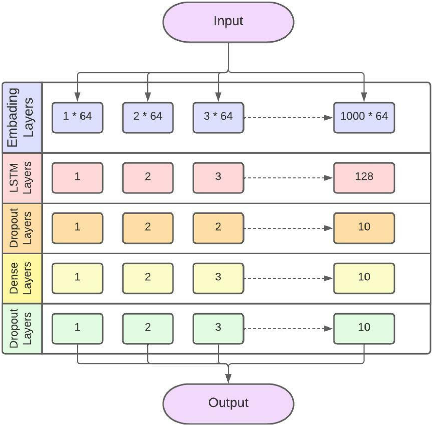
LSTM layered structure model for identification of sarcoma cancer.

The proposed LSTM has an embedding layer. Embedding layer is used to convert the input into a fixed length vector of defined size. The vocabulary size is 1000 and the length of the word vector is 64. The second layer is the LSTM layer. The LSTM layer has 128 neurons in the output layer. Further, two dropout layers are also added. Subsequently, 10% neurons are kept off to avoid overfitting. A dense layer is used with 10 neurons. Stochastic Gradient Descent (SGD) is used in LSTM as an optimizer. Sigmoid is used as an activation function. The Sparse Categorical Cross Entropy (SCCE) function is used to minimize the loss.

The gate in LSTM is responsible for the regulation of information from one cell to another cell. Different activation functions are applied in each gate.^{50, 51} Figure 7 presents the working model of gates in LSTM.⁵²

Fig. 7.

A simple LSTM cell structure.

where $x_{t}$ is the input and $h_{t}$ is the output at specific time t. $f_{t}$ represents forget gate, $i_{t}$ and $o_{t}$ represent input and output gate respectively. Every cell of LSTM has three inputs $x_{t}, h_{t - 1}, C_{t - 1}$ and has two outputs as $h_{t}$ and $C_{t}$ . Equation 13, 14, 15, 16, 17, 18 explain LSTM.

i_{t} = σ (x_{t} A^{i} + h_{t - 1} B^{i}

(13)

f_{t} = σ (x_{t} A^{f} + h_{t - 1} B^{f}

(14)

o_{t} = σ (x_{t} A^{o} + h_{t - 1} B^{o})

(15)

C_{t}^{'} = \tanh (x_{t} A^{c} + h_{t - 1} B^{c})

(16)

C_{t} = σ (f_{t} * C_{t - 1} + i_{t} * C_{t}^{'}

(17)

h_{t} = \tanh (C_{t}) * o_{t}

(18)

where

h_{t - 1}

is the previous data cell output,

C_{t - 1}

is the previous cell memory,

C_{t}

is the current cell memory? While A and B are the weights for the forget, input and output gate.

Gated recurrent unit (GRU)

Another DL algorithm used in this proposed study is GRU. It works in a similar fashin as LSTM does, but it uses less parameters and a smaller number of gates. It performs better then LSTM with smaller training data. Another benefit of using GRU over LSTM is that GRU is simpler than LSTM and provide good performance. GRU uses only two gates, reset gate and update gate in the cell.⁴⁹ The layered structure of GRU in sarcoma cancer detection is explained in Figure 8.

Fig. 8.

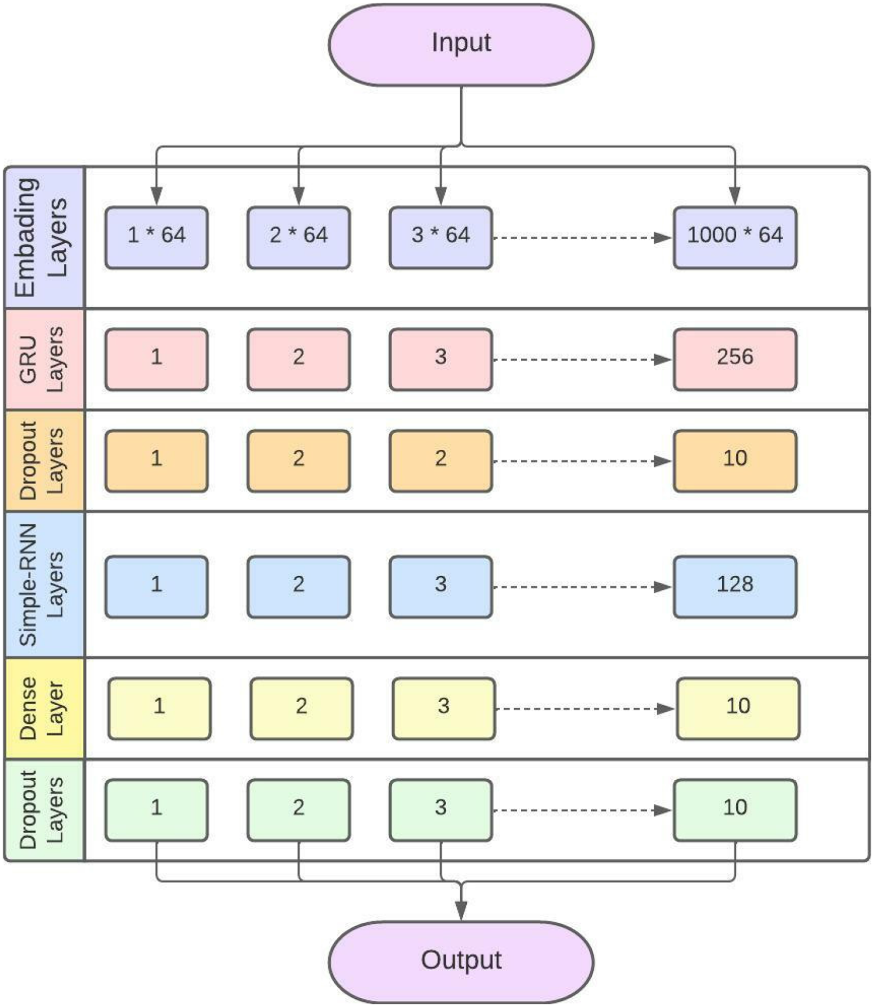
GRU layered structure model for identification of sarcoma cancer.

The proposed GRU has 1 embedding layer. Embedding layer is used to convert the input into a fixed length vector of defined size. vocabulary size is 1000 and the length of word vector is 64. The second layer is GRU layer. The GRU layer has 256 neurons in output layer. One simple RNN layer is also added with 128 neurons. Further, two dropout layers are also added. Subsequently, 10 percent neurons are kept off to avoid overfitting. A dense layer is used with 10 neurons. SGD is used in GRU as an optimizer. Sigmoid is used as an activation function. SCCE function is used to minimize the loss.

The reset gate of GRU decides how much past information is neglected and the update gate decides how much past information is to be used. Figure 9 explains the cell structure of GRU.⁵³

Fig. 9.

A simple GRU cell structure.

Equations 19, 20, 21, and 22 explain the GRU working process.

r_{t} = σ (x_{t} A^{r} + h_{t - 1} B^{r}

(19)

z_{t} = σ (x_{t} A^{z} + h_{t - 1} B^{z}

(20)

h_{t}^{'} = \tanh (r_{t} * h_{t - 1} A + x_{t} B)

(21)

h_{t} = (1 - z_{t}) * h_{t}^{'} + z_{t} * h_{t - 1})

(22)

Equations (19) and (20) $r_{t}$ represents the reset gate and $z_{t}$ is the update gate. GRU takes less computational time than LSTM.⁵⁴

Bi-Directional LSTM

Finally, the DL technique used in the proposed study is Bi-directional LSTM.⁵⁵ A Bi-directional LSTM uses two LSTM cells, one in the forward direction and one in the backward direction that are related to a single output.

The proposed Bi-directional LSTM has one embedding layer. The embedding layer is used to convert the input into a fixed-length vector of defined size. Similarly, the vocabulary size is 1000 and the length of the word vector is 64. The second layer is the LSTM layer. The LSTM layer has 64 neurons in the output layer. Three dropout layers are added. In the first dropout layer, 20% neurons are kept off. In the second dropout layer, 20% neurons are kept off and in the third dropout layer, 10% neurons are kept off to avoid overfitting. Furthermore, two dense layers are also used. The first dense layer has 64 neurons, and the second layer has 10 neurons. Adaptive Moment Estimation (ADAM) is used in bi-directional LSTM as an optimizer. Sigmoid is used as an activation function. The Binary Cross Entropy function is used to minimize the loss.

This process does not need any past knowledge it learns itself by moving in forward and backward directions.⁵⁶ The proposed Bi-directional LSTM is explained in Figures 10 and 11.

Fig. 10.

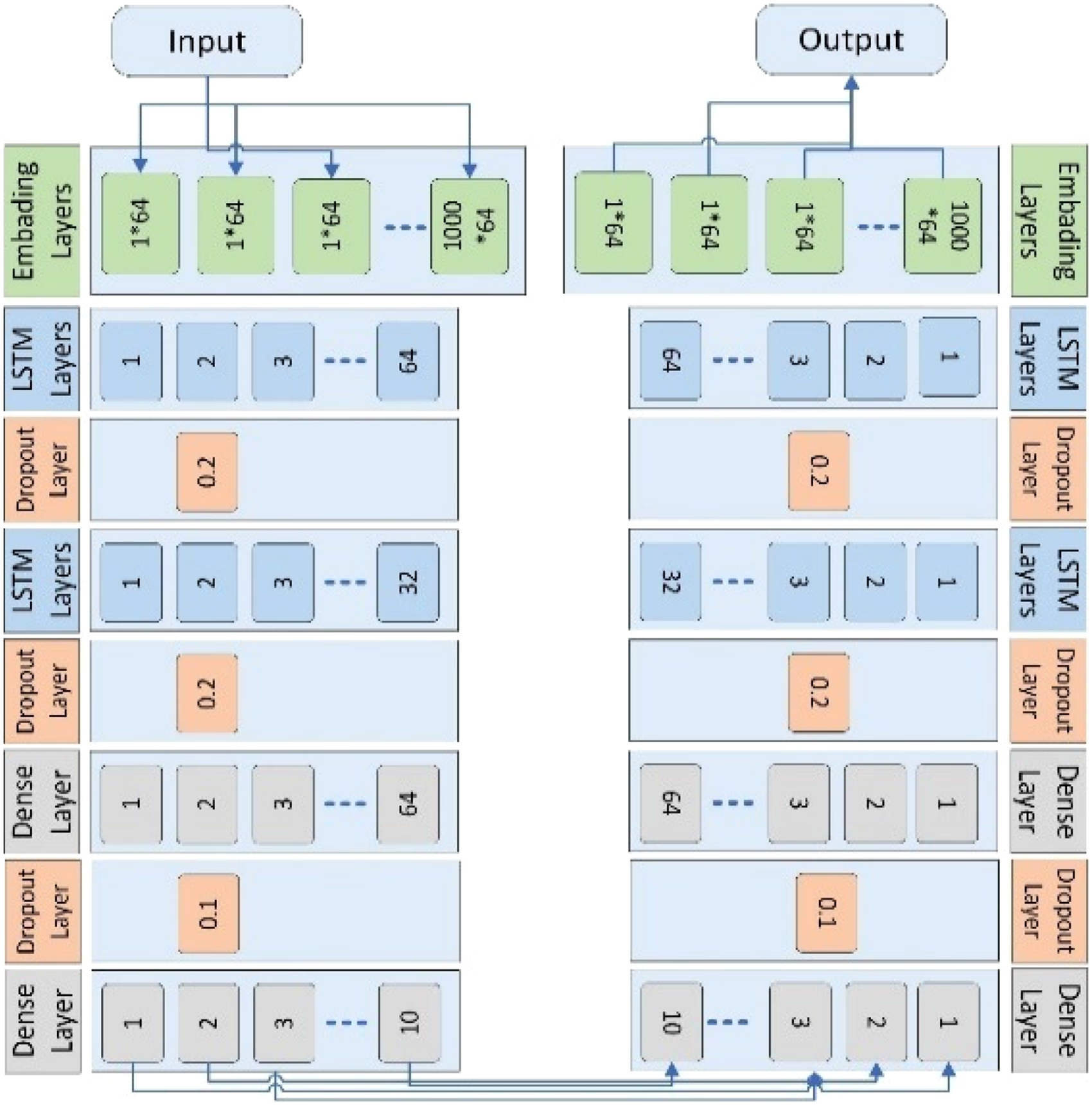
Bi-directional LSTM layered structure model that depicts both directions.

Fig. 11.

Bi-directional LSTM layered structure model for identification of sarcoma cancer.

The models are trained using 20 epochs (20 iterations of feed-forward and feed backward). The performance of the DL techniques is evaluated using AUC, precision, F1 score, recall, Cohen's kappa, Specificity, Sensitivity, Mathew's correlation coefficient, loss, and Accuracy.^57,58 The equations (23), (24), (25), and (26) describe sensitivity, specificity, accuracy, and Mathew's correlation coefficient respectively.

Sensitivity = \frac{TP}{TP + FN}

(23)

Specificity = \frac{TN}{TN + FP}

(24)

Accuracy = \frac{TP + TN}{TP + FP + FN + TN}

(25)

MCC = \frac{(TP \times TN) - (FP \times FN)}{\sqrt{(TP + FP) (TP + FN) (TN + FP) (TN + FN})}

(26)

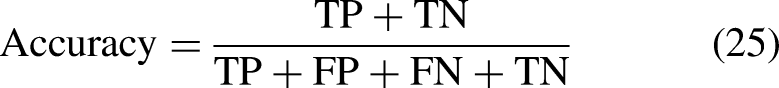
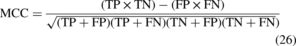
In these equations:

TN = All the true negative values

TP = All the true positive values from the dataset

FN = False Negative values

FP = False positive values

For the proposed study Sensitivity refers to the ability of tests that truly identify the sarcoma cancer while specificity mentions to the ability of the tests that truly identify those who did not have sarcoma cancer in the dataset.⁵⁹ In the equations

T P + F N

represents all subjects with a given conditions. While

T N + F P

is all the subjects without the given conditions.

T P + F P

is the total number of subjects with positive test and

T N + F N

is the subjects with the negative results.⁶⁰ A confusion matrix is a technique used for summarizing the algorithm.^61,62 TN are True Negative values, TP are True Positive values, FN are False Negative, and FP are False Positive values that are represented in the confusion matrix.

Results

The dataset of sarcoma cancer is preprocessed and then processed so that the main features of the balanced data are extracted. The DL algorithms are then applied to the extracted data. To validate the performance of DL algorithms independent set test, self-consistency test, and 10-fold cross-validation test are applied. The results of these validation techniques are explained in this section.

Self-consistency testing

Self-consistency test is the testing technique used for testing the DL algorithm. In the self-consistency test, 100% data is used for training and testing purposes. In self-consistency test the whole dataset is used for both training and testing. Bi-directional LSTM has a very minimum loss. Whereas, LSTM, GRU, and Bidirectional LSTM achieved very good accuracy in the self-consistency test as shown in Table 3.

The ROC curve of the LSTM algorithm is shown in Figure 12.

Fig. 12.

ROC curve of LSTM using self-consistency test.

The accuracy and loss curve of LSTM in the self-consistency test is shown in Figures 13 and 14.

Fig. 13.

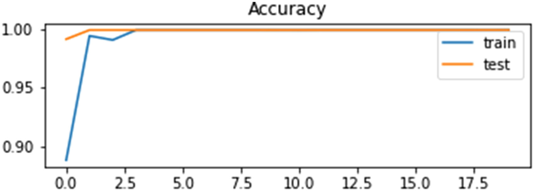
Accuracy curve of LSTM using self-consistency test.

Fig. 14.

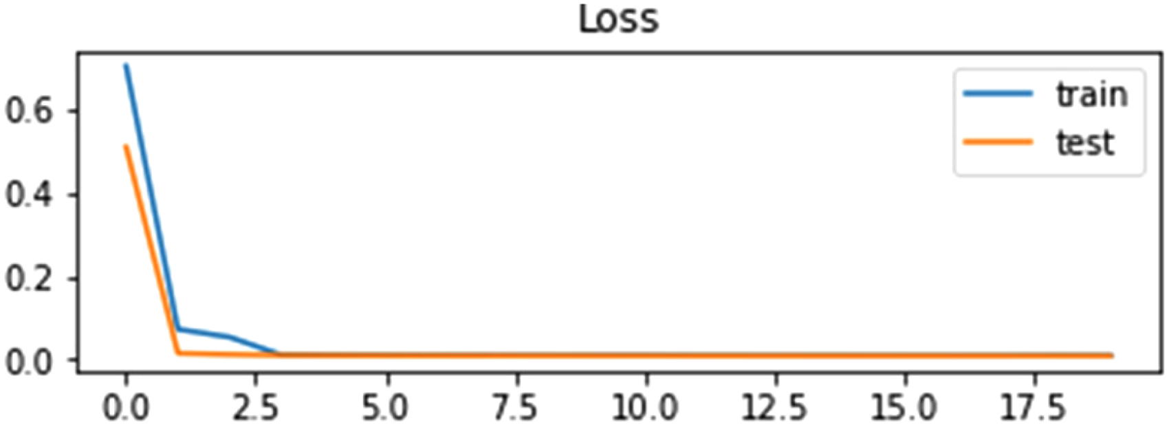
Loss curve of LSTM using self-consistency test.

Figures 13 and 14 illustrate that the accuracy of the LSTM algorithm is increasing gradually at the same time the loss curve value is decreasing gradually for training and testing data.

In the layered framework of RNN, different types of convolutional filters are applied to the extracted data. The sequential model is used here.

The ROC curve of the GRU algorithm while self-consistency test is applied on it is shown in Figure 15.

Fig. 15.

ROC curve of GRU using self-consistency test.

Accuracy and loss curve of GRU in the self-consistency test is shown in Figures 16 and 17.

Fig. 16.

Accuracy curve of GRU using self-consistency test.

Fig. 17.

Loss curve of GRU using self-consistency test.

The ROC curve of bi-directional LSTM is explained in Figure 18.

Fig. 18.

ROC curve of bi-directional LSTM using self-consistency test.

The combined ROC curve of LSTM, GRU, and Bi-directional LSTM when self-consistency test applied on them is illustrated in Figure 19.

Fig. 19.

Combined ROC curve of LSTM, GRU, and bi-directional LSTM using self-consistency testing.

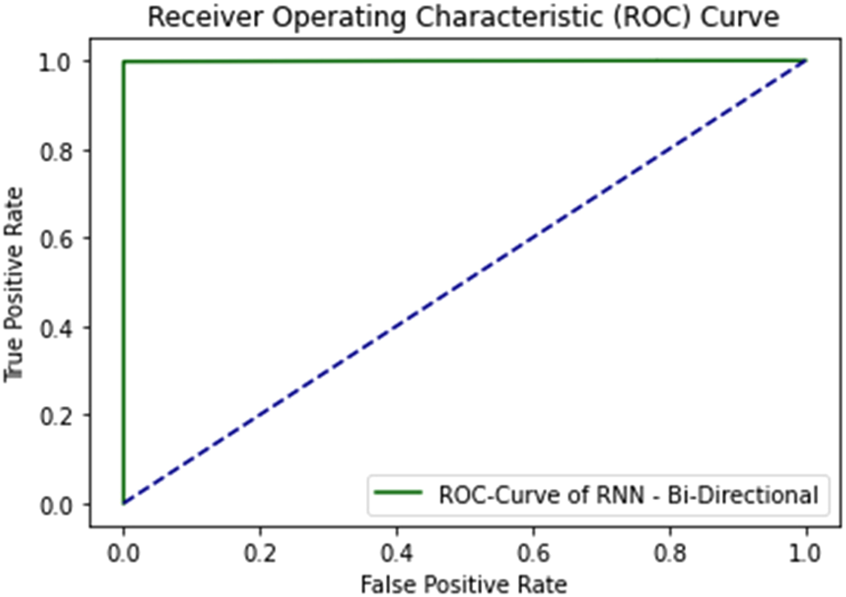
All three DL algorithms give an AUC Value of 1.0 considered as excellent results according to AUC accuracy classification.⁶³

Independent set testing

Another validation technique used for the proposed work is independent set testing. The values are extracted from the confusion matrix to determine the precision of the model. This test is considered as the basic performance measuring method for the proposed model. Where 80% of the dataset is used for training the algorithm while 20% is used for testing purposes.

Table 4 illustrates the results of the independent set test on LSTM, GRU, and bi-directional LSTM.

Table 4.

Results of independent set testing.

	LSTM	GRU	Bidirectional LSTM
AUC	1.00	1.00	1.00
Sn	99%	99%	89%
Sp	98%	98%	90%
MCC	0.99	0.99	0.90
Acc	99%	99%	92%
Loss	0.0074	0.0073	0.0075

LSTM: long and short-term memory; GRU: gated recurrent unit; AUC: Area Under the Curve.

LSTM uses the same parameters with the same layer filters in all the testing techniques. The ROC curve of the LSTM algorithm is shown in Figure 20.

Fig. 20.

ROC curve of LSTM using the independent set test.

The ROC curve of LSTM gives the AUC value 1.00 on the graph. The accuracy and loss curve of LSTM in independent set testing is shown in Figures 21 and 22.

Fig. 21.

Accuracy curve of LSTM using independent set testing.

Fig. 22.

Loss curve of LSTM using independent set testing.

Figures 21 and 22 illustrate that the accuracy is increasing gradually at the same time the loss curve value is decreasing gradually for training and testing data. The ROC curve of the GRU algorithm while independent set test is applied on it is shown in Figure 23.

Fig. 23.

ROC curve of GRU using independent set test.

The accuracy and loss curve of GRU shows that the accuracy of the model is increasing with every iteration in the meantime the loss of the model decreases gradually forming the curve as shown in Figures 24 and 25.

Fig. 24.

Accuracy curve of GRU using independent set test.

Fig. 25.

Loss curve of GRU using independent set test.

The accuracy of the training set is represented by a blue line and the accuracy of the testing dataset is represented by a yellow line. The GRU algorithm gives an accuracy of 99% with an AUC value of 1 which is considered as an excellent result for the identification of sarcoma cancer.

Figure 26 illustrates the ROC of bi-directional LSTM using an independent set testing technique.

Fig. 26.

ROC curve of bidirectional LSTM using independent set test.

The accuracy and loss curve of bidirectional LSTM in the independent set test are shown in Figures 27 and 28.

Fig. 27.

Accuracy curve of bidirectional LSTM using self-consistency test.

Fig. 28.

Loss curve of bi-directional LSTM using self-consistency test.

The combined ROC curve of LSTM, GRU, and Bi-directional LSTM when an independent set test is applied to them is illustrated in Figure 29.

Fig. 29.

Combined ROC curve of LSTM, GRU and bidirectional LSTM using the independent set test.

10-Fold cross-validation test

In the 10-Fold cross-validation (10-FCV) testing technique, the data is equally subsampled into 10 groups. divide the training set into 10 partitions and then treat each of them in the validation set, training the model and then average generalization performance across the 10-folds to make choices about hyper-parameters and architecture.⁶⁴

Figure 30 shows the working process of the 10-fold cross-validation technique.

Fig. 30.

Working process of 10-fold cross-validation.

Table 5 represents the results of the 10-fold cross-validation technique.

Table 5.

Results of 10-fold cross-validation.

	LSTM	GRU	Bidirectional LSTM
AUC	1.00	1.00	1.00
Sn	100%	100%	90%
Sp	99%	99%	50%
MCC	0.99	0.99	0.92
Acc	99%	99%	96%
Loss	0.0083	0.0079	0.0088

LSTM: long and short-term memory; GRU: gated recurrent unit; AUC: Area Under the Curve.

The ROC curve of the LSTM algorithm when the 10-FCV test is applied to it is shown in Figure 31.

Fig. 31.

ROC curve of LSTM using 10-FCV.

Figure 31 shows that there are 10 results for LSTM on each iteration because 10-fold cross-validation data is divided into 10 groups and each group is trained and tested separately.

The ROC curve of the GRU algorithm while a 10-fold cross-validation test is applied to it is shown in Figure 32.

Fig. 32.

ROC curve of GRU using 10-FCV test.

Figure 33 illustrates the ROC of bi-directional LSTM using a 10-fold cross-validation testing technique.

Fig. 33.

ROC curve of bidirectional-LSTM using 10-FCV test.

Comparison

The proposed model is compared with the latest state-of-the-art models based on the independent set test. The results of the proposed model are very good in comparison to the state-of-the-art work as shown in Table 6. The results are further discussed in detail in the discussion section.

Table 6.

Comparison of the proposed model with state-of-the-art models based on the independent set test.

	Proposed models			Previous work [29]			Previous work [33]			Previous work [67]
	LSTM	GRU	Bi-LSTM	RF	SVM	NN	RF	SVM	NN	RNN	LSTM	GRU
Acc%	99	99	92	92.48	86.81	88.23	100	94.3	64.2	73.1	78.4	77.2
Sn%	99	99	89	84.12	71.66	81.39	100	100	92.9	73.3	79.9	78.7
Sp%	98	98	90	96.12	99.54	83.01	100	83.1	7.0	73.1	78.4	77.2
MCC	0.99	0.99	0.90	0.814	0.552	0.601	1.0	0.9	0.01	NA	NA	NA

LSTM: long and short-term memory; GRU: gated recurrent unit; RNN: Recurrent Neural Network.

Discussion

This work proposed a framework based on three DL models such as LSTM, GRU, and bi-directional LSTM. The proposed framework is a robust in-silico technique for the identification of mutations in sarcoma cancer. This proposed framework is a computationally intelligent predictor in comparison to the state of the artwork. Mutation information and normal gene sequences are obtained through web scrapping code written in python. Then mutated sequences are generated by incorporating the mutation information into normal gene sequences and thus a benchmark dataset acquisition framework is developed. Then a feature extraction framework is developed to extract useful features to help the proposed DL framework in learning the hidden patterns in the data and to yield better results. Statistical moments, PRIM, RPRIM, FV, AAPIV, and RAAPIV are calculated to form feature vectors. The performance of LSTM, GRU, and bi-directional LSTM is shown in Tables 3, 4, and 5. GRU performed the best performance among LSTM, GRU, and bi-directional LSTM.

Three test methods such as self-consistence test, independent set test, and 10-fold cross-validation test are used to validate the performance of proposed DL techniques. 100% data is used in both training and testing in self-consistence tests to know about the training accuracy of the model. 80% data is used for training and 20% data is used for testing in independent set test. Unseen data is provided as testing to independent set test. The dataset is divided into 10 folds and the model is applied as leave one out approach and the average accuracy is obtained in 10-fold cross-validation test.

Thus, the suitability of the proposed model is discussed based on its performance. The proposed framework helps to identify mutations in sarcoma cancer efficiently and accurately. It is clear from the results that the proposed framework is a potent computational identifier for the rapid and cost-effective detection of mutations in sarcoma cancer.

The results and comparison of LSTM, GRU, and Bi-directional LSTM are presented in Tables 3, 4, and 5, respectively. Numerous evaluation metrics are tabulated such as sensitivity, specificity, MCC, accuracy, and loss for the self-consistency test, independent set test, and 10-fold cross-validation test. The proposed algorithms yield prolific results. The accuracy on average is almost 99%. The performance of LSTM, GRU, and Bi-directional LSTM is almost similar in self-consistency test. The performance of GRU is high according to the independent set test and 10-fold cross-validation test.

The loss of the proposed models is very low and almost negligible as shown in Figures 22, 25, and 28 respectively. It is also clear from the ROC curves that the proposed models performed very well as shown in Figures 12, 15, 18, 19, 20, 23, 26, 29, 31, 32, and 33 respectively.

The limitations of the proposed model are that it is trained and tested only on sarcoma cancer to identify mutations pertinent to sarcoma. In the future, this work will be extended to identify other types of diseases while exploring more computational models like ensemble and DL models.

Conclusion

Sarcoma is a cancer of bones and soft tissues. It is mostly present in the arms and legs of humans. The proposed work shows the best possible results for the early detection of sarcoma cancer using RNN DL algorithms. There are three DL algorithms LSTM, GRU, and bi-directional LSTM used for the identification of a mutation in sarcoma cancer. All the algorithms give an average accuracy of 99.8% with an AUC value of 1.00. These are the best results for the identification of sarcoma cancer till date.

The Accuracy, AUC, Loss, Sensitivity, Specificity, and Mathew's correlation coefficient of the independent set test, self-consistency test and10-fold cross-validation test were calculated and shown in Tables 3, 4, and 5. These are the best approaches for detecting sarcoma cancer at its early stages till date.

In future, this work will be extended to identify other types of diseases and an ensemble DL model will also be proposed.

Footnotes

Acknowledgments:

The researchers would like to thank the Deanship of Scientific Research, Qassim University for funding the publication of this project.

Contributorship

The manuscript was prepared by AAS, FA, and TA. The implementation of this study is done by AAS and YDK. The manuscript was reviewed and supervised by YDK. All authors contributed to the text in the manuscript and reviewed and approved the final version of the manuscript.

Guarantor:

AAS.

Ethical approval:

Ethical approval was not required for this study.

Declaration of conflicting interests:

The authors declared no potential conflicts of interest with respect to the research, authorship, and/or publication of this article.

Funding:

The authors received no financial support for the research, authorship, and/or publication of this article.

ORCID iDs

Fahad Alturise

Tamim Alkhalifah

References

Min

Lee

Yoon

. Deep learning in bioinformatics. Brief Bioinform 2017; 18: 851–869.

Zhang

Liu

. Bioinformatics. Brenner’s Encycl Genet Second Ed 2013: 338–340. doi: 10.1016/B978-0-12-374984-0.00155-8.

Koonin

. Computational genomics. pp. 155–158.

Timpson N. Bioinformatics and Functional Genomics. Pevsner J. Chichester: John Wiley & Sons Inc, 2003, pp. 753,£ 58.50 ISBN: 0-471-21004-8. International Journal of Epidemiology 2004; 33(4): 913–914.

Alterations

. 4.8: Mutation Types - Biology LibreTexts, pp. 10–12, [Online]. Available: https://bio.libretexts.org/Bookshelves/Introductory_and_General_Biology/Book%3A_Introductory_Biology_(CK-12)/04%3A_Molecular_Biology/4.08%3A_Mutation_Types [Accessed 19 April 2022].

Zeiger

Consulting

Hill

. 3. 10 GenAetic Toxicology Testing. 2010.

Genetic Mutations- Definition, Types, Causes and Examples – Genetic Education. https://geneticeducation.co.in/genetic-mutations-definition-types-causes-and-examples/ (accessed Nov. 10, 2021).

AACR. AACR Cancer Progress Report. 2020.

Shujaat

Aslam

Noreen

, et al. Intelligent and integrated framework for exudate detection in retinal fundus images. Intelligent Automation & Soft Computing 2021; 30: 663–672.

10.

Saeed

Shah

Ehsan

, et al. Automated facial expression recognition framework using deep learning. J Healthc Eng 2022; 2022: 1–11. Available: 10.1155/2022/5707930 [Accessed 24 June 2022].

11.

Vishwanathan

SVN

Murty

. SSVM: a simple SVM algorithm. Proc Int Jt Conf Neural Networks 2002; 3: 2393–2398.

12.

Myles

Feudale

Liu

, et al. An introduction to decision tree modeling. J Chemom 2004; 18: 275–285.

13.

Alaoui

EAA

Tekouabou

SCK

Hartini

, et al. Improvement in automated diagnosis of soft tissues tumors using machine learning. Big Data Min Anal 2021; 4: 33–46.

14.

, et al. Feature selection: a data perspective. ACM Comput Surv 2017; 50: 1–45. doi: 10.1145/3136625.

15.

Hossain

Rahaman

. Bone cancer detection classification using fuzzy clustering neuro fuzzy classifier. 4th Int. Conf. Electr. Eng. Inf. Commun. Technol. iCEEiCT 2018, no. September, pp. 541–546, 2019, doi: 10.1109/CEEICT.2018.8628164.

16.

Foersch

, et al. Deep learning for diagnosis and survival prediction in soft tissue sarcoma. Ann Oncol 2021; 32: 1178–1187.

17.

hui Ren

jun Deng

hua Yuan

, et al. An immune-related gene signature for determining Ewing sarcoma prognosis based on machine learning. J Cancer Res Clin Oncol 2021; 147: 153–165.

18.

Barupal

Fiehn

. Generating the blood exposome database using a comprehensive text mining and database fusion approach. Environ Health Perspect 2019; 127: 2825–2830.

19.

Jeong

Lin

Chen

. On position-specific scoring matrix for protein function prediction. IEEE/ACM Trans Comput Biol Bioinf 2011; 8: 308–315.

20.

Caragea

Silvescu

Mitra

. Protein sequence classification using feature hashing. In: Proceedings of the IEEE International Conference on Bioinformatics and Biomedicine (BIBM’11), Atlanta, GA, USA, pp. 538–543, Nov. 2011.

21.

Asgari

Mofrad

RKM

. Continuous distributed representation of biological sequences for deep proteomics and genomics. PloS one 2015; 10: 1–15.

22.

Vazhayil

. DeepProteomics: Protein family classification using Shallow and Deep Networks. arXiv.org, 2022.

23.

Gene: H4C7 (ENSG00000275663) - Summary - Homo_sapiens - Ensembl genome browser 105. Asia.ensembl.org, 2022. [Online]. Available: http://asia.ensembl.org/Homo_sapiens/Gene/Summary?g=ENSG00000275663&db=core. [Accessed: 01- Mar- 2022].

24.

IntOGen - Cancer Mutations Browser. Intogen.org, 2022. [Online]. Available: https://www.intogen.org/. [Accessed: 01- Mar- 2022].

25.

Waks

Weissbrod

Carmeli

, et al. Driver gene classification reveals a substantial overrepresentation of tumor suppressors among very large chromatin-regulating proteins. Sci Rep 2016; 6: 1–12.

26.

Generating Word Cloud in Python - GeeksforGeeks. GeeksforGeeks, 2022. [Online]. Available: https://www.geeksforgeeks.org/generating-word-cloud-python/#:∼:text=Word%20Cloud%20is%20a%20data,highlighted%20using%20a%20word%20cloud. [Accessed: 19 April- 2022].

27.

Kaur

Gosain

. Comparing the behavior of oversampling and undersampling approach of class imbalance learning by combining class imbalance problem with noise. Adv Intell Syst Comput 2018; 653: 23–30.

28.

Shah

Khan

. Identification of 4-carboxyglutamate residue sites based on position based statistical feature and multiple classification. Sci Rep 2020; 10: 2–11.

29.

Feature extraction: A survey | IEEE Journals & Magazine | IEEE Xplore. https://ieeexplore.ieee.org/abstract/document/1449207/authors#authors (accessed Aug. 28, 2021).

30.

Malebary

Khan

. Evaluating machine learning methodologies for identification of cancer driver genes. Sci Rep 2021; 11: 1–13.

31.

Sohail

Shabbir

Sohil

. Imputation of missing values by using raw moments. Stat Transit 2019; 20: 21–40.

32.

Butt

Khan

. CanLect-Pred: a cancer therapeutics tool for prediction of target cancerlectins using experiential annotated proteomic sequences. IEEE Access 2020; 8: 9520–9531.

33.

Shahid

Ilyas

Hussain

, et al. ORI-Deep: improving the accuracy for predicting origin of replication sites by using a blend of features and long short-term memory network. Brief Bioinform 2022; 23.

34.

Allehaibi

Daanial Khan

Khan

. iTAGPred: a two-level prediction model for identification of angiogenesis and tumor angiogenesis biomarkers. Appl Bionics Biomech 2021; 2021: 1–15.

35.

Ashraf

Khan

Shoaib

, et al. βLact-Pred: a predictor developed for identification of beta-lactamases using statistical moments and PseAAC via 5-step rule. Comput Intell Neurosci 2021; 2021: 1–10.

36.

Malebary

Alzahrani

Khan

. A comprehensive tool for accurate identification of methyl-glutamine sites. J Mol Graphics Modell 2022; 110: 108074.

37.

Nour

Salem

Habashy

. “ILipo-PseAAC: identification of lipoylation sites using statistical moments and general PseAAC. Computers, Materials & Continua 2022; 71: 215–230.

38.

Arif

, et al. StackACPred: prediction of anticancer peptides by integrating optimized multiple feature descriptors with stacked ensemble approach. Chemom Intell Lab Syst 2022; 220: 104458.

39.

Alghamdi

Alzahrani

Ullah

, et al. 4mC-RF: improving the prediction of 4mC sites using composition and position relative features and statistical moment. Anal Biochem 2021; 633: 114385.

40.

Khan

Naseer

, et al. iSUMOK-PseAAC: prediction of lysine sumoylation sites using statistical moments and chou’s PseAAC. PeerJ 2021; 9: e11581.

41.

Malebary

Khan

. Protopred: advancing oncological research through identification of proto-oncogene proteins. IEEE Access 2021; 9: 68788–68797.

42.

Malebary

Daanial Khan

. “Identification of antimicrobial peptides using chou’s 5 step rule. Computers, Materials & Continua 2021; 67: 2863–2881.

43.

Naseer

Ali

Khan

, et al. iGluK-Deep: computational identification of lysine glutarylation sites using deep neural networks with general pseudo amino acid compositions. J Biomol Struct Dyn 2021: 1–14.

44.

Akmal

Rasool

Khan

. Prediction of N-linked glycosylation sites using position relative features and statistical moments. PLoS One 2017; 12: 1–21..

45.

Lecun

Bengio

Hinton

. Deep learning. 2015, doi: 10.1038/nature14539.

46.

Vinayakumar

Alazab

Srinivasan

, et al. A visualized botnet detection system based deep learning for the internet of things networks of smart cities. IEEE Trans Ind Appl 2020; 56: 4436–4456.

47.

Vinayakumar

Alazab

Soman

, et al. Deep learning approach for intelligent intrusion detection system. IEEE Access 2019; 7: 41525–41550.

48.

Ravi

Alazab

Srinivasan

, et al. Adversarial defense: DGA-based botnets and DNS homographs detection through integrated deep learning. IEEE Trans Eng Manage 2021: 1–18. doi: 10.1109/TEM.2021.3059664.

49.

Rengasamy

Jafari

Rothwell

, et al. Deep learning with dynamically weighted loss function for sensor-based prognostics and health management. Sensors (Switzerland) 2020; 20: 1–21. doi: 10.3390/s20030723.

50.

, et al. Recent advances in convolutional neural networks. Pattern Recognit 2018; 77: 354–377.

51.

Lin

Shen

. Research on convolutional neural network based on improved Relu piecewise activation function. Procedia Comput Sci 2018; 131: 977–984.

52.

Varsamopoulos

Bertels

Almudever

. Designing neural network based decoders for surface codes Accelerated BWA-MEM View project Hartes View project Designing neural network based decoders for surface codes. arXiv:1811.12456 [quant-ph], no. November, pp. 1–12, 2018, [Online]. Available: https://www.researchgate.net/publication/329362532.

53.

Mateus

Mendes

Farinha

, et al. Comparing LSTM and GRU models to predict the condition of a pulp paper press. Energies 2021; 14: 1–21.

54.

Gao

Glowacka

. Deep gate recurrent neural network. J Mach Learn Res 2016; 63: 350–365.

55.

Graves

Schmidhuber

. Framewise phoneme classification with bidirectional LSTM and other neural network architectures. Neural Netw 2005; 18: 602–610.

56.

Basaldella

Antolli

Serra

, et al. Bidirectional LSTM Recurrent Neural Network. Pp. 345–353, 2018. doi: 10.1007/978-3-319-46681-1.

57.

Van Stralen

Stel

Reitsma

, et al. Diagnostic methods I: sensitivity, specificity, and other measures of accuracy. Kidney Int 2009; 75: 1257–1263.

58.

Alford

Nicoletti

Derzon

, et al. Sensitivity, specificity, and predictive values: foundations, pliabilities, and pitfalls in research and practice. Artic 307 1 Public Heal 2017; 5: 07.

59.

Lalkhen

McCluskey

. Clinical tests: sensitivity and specificity. Contin Educ Anaesthesia, Crit Care Pain 2008; 8: 221–223..

60.

Zhu

Zeng

Wang

. Sensitivity, specificity, accuracy, associated confidence interval and ROC analysis with practical SAS^® implementations. Northeast SAS Users Gr 2010 Heal Care Life Sci 2010; 19: 1–9.

61.

Visa Sofia

. Confusion matrix-based feature selection Sofia visa. ConfusionMatrix-based Featur Sel Sofia 2011; 710: 8.

62.

Analysis

Error

Reliability

, et al. Foundations of data imbalance and solutions for a data democracy Data analysis and machine learning tools in MATLAB and Python Fake news in social media recognition using Modified Long Short-Term Memory network Handling of Feature Space Complexity for. pp. 2018–2020, 2020.

63.

Cortes

Mohri

. AUC Optimization vs. Error rate minimization. Adv Neural Inf Process Syst 2004; 16.

64.

Adams

. Model Selection and Cross Validation Evaluation Hygiene: the Train / Test Split. pp. 1–8.

Evaluation of deep learning techniques for identification of sarcoma-causing carcinogenic mutations

Abstract

Keywords

Introduction

Literature review

Materials and methods

Data acquisition framework

Feature extraction framework

Statistical moments

Position relative incidence matrix

Reverse position relative incidence matrix

Frequency vector

Accumulative absolute position incidence vector

Reverse accumulative absolute position incidence vector (RAAPIV)

Prediction algorithm

LSTM network

Gated recurrent unit (GRU)

Bi-Directional LSTM

Results

Self-consistency testing

Independent set testing

10-Fold cross-validation test

Comparison

Discussion

Conclusion

Footnotes

Acknowledgments:

Contributorship

Guarantor:

Ethical approval:

Declaration of conflicting interests:

Funding:

ORCID iDs

References