Sage Journals: Discover world-class research

Abstract

Mazumder investigates the long-term effect of protest on political attitudes. He finds that whites have more liberal views on race and are more likely to be Democrats in counties where Civil Rights protest was reported in the early 1960s. The analysis omits a crucial predictor of protest and of racial attitudes: college education. We include the proportion of adults with a college degree and the number of college students at the county level. The inclusion of these variables, along with some other contextual variables from the original dataset, cuts the effect of protest by about half. Protest is no longer statistically significant in eight out of nine combinations of outcome variables and protest measures. The size of the effect remains trivial when we shift analysis from the county to the individual level. Even accounting for the individual’s own education, the county’s proportion of college graduates is strongly associated with racial liberalism. This finding emphasizes the importance of education as a contextual variable. Our conclusion highlights two methodological lessons. First, causal inference should be paired with sustained historical inquiry that specifies plausible mechanisms. Second, statistical tests for sensitivity can induce complacency about the risk of confounding.

Keywords

Social movements race collective protest

Introduction

Does collective protest shift public opinion? Several recent studies demonstrate a causal effect. Most obviously, protest can induce more favorable attitudes to the cause (Andrews et al., 2016; Branton et al., 2015; Madestam et al., 2013; Tertytchnaya and Lankina, 2020; Wallace et al., 2014). Protest can also have the reverse effect, polarizing opinion (Motta 2018) or even eroding support for democracy (Ketchley and El-Reyyes, 2020). All these studies identify effects over the short term, from a few days to a few years. Mazumder (2018) is more ambitious, investigating whether Civil Rights protest in the early 1960s affected public opinion early in the 21st century. He finds that “whites from counties that experienced historical civil rights protests are more likely to identify as Democrats and support affirmative action, and less likely to harbor racial resentment against blacks” (Mazumder, 2018: 922). Dependent variables are derived from the Cooperative Congressional Election Study (CCES) in 2006 and 2008–2011. White respondents are aggregated by county. The key independent variable is a binary indicator for whether one newspaper reported any protest for Civil Rights between 1960 and 1965. The main analysis controls for five county characteristics measured in 1960 or before. Mazumder’s study complements a burgeoning literature on the long-term legacy of political violence (Rozenas and Zhukov, 2019; Voigtländer and Voth, 2012). It also augments an established literature on the historical legacy of slavery, lynching, and anti-black mobilization in the American South (Acharya et al., 2016; Andrews, 1997; McVeigh et al., 2014).

This paper scrutinizes Mazumder’s findings. The key independent variable is subject to significant measurement error. The analysis omits a crucial predictor of protest and of racial attitudes: college education. When we include the proportion of adults with a college degree and the number of students at the county level, along with other control variables from the original dataset, the effect of protest is reduced by about half. It is no longer statistically significant in eight out of nine combinations of outcome variables and protest measures. When we analyze individual respondents, controlling for their education and other characteristics, the county’s college education and student numbers in 1960 are still strongly associated with racial liberalism. In short, there is insufficient evidence to support any causal relationship between the incidence of Civil Rights protest and variation in whites’ racial attitudes in the early 21st century. Instead, the reanalysis demonstrates the importance of education in predicting social attitudes, at the contextual as well as the individual level. Our conclusion highlights two methodological lessons. First, causal inference should be paired with sustained historical inquiry that specifies plausible mechanisms. Second, statistical tests for sensitivity can induce complacency about the risk of confounding.

Measurement error and omitted variables

Mazumder’s key independent variable—the occurrence of protest at the county level—is derived from a single newspaper, the New York Times. By contrast, other recent studies of the effects of protest utilize event data from multiple newspapers (Ketchley and El Reyyes, 2020), often complemented by records from movement organizations (Madestam et al., 2013). The vast majority of protest events are never reported in the New York Times—a recent estimate is under 5% (Beyerlein et al., 2018). Therefore many counties will be erroneously classified as experiencing no protest. The magnitude of this problem is indicated by comparing a comprehensive list of Southern states with sit-ins—where blacks physically occupied spaces from which they were excluded—during the spring of 1960 (Andrews and Biggs, 2006; Biggs and Andrews, 2015). Of 64 counties that experienced these especially disruptive and hence visible events, 20 had no Civil Rights protest of any kind reported by the New York Times over the same period. Sociologists who study the reporting of protest conclude that newspaper data have “very serious flaws” and so scholars “need to spend more time and print space thinking about how these shortcomings may affect their results” (Ortiz et al., 2005: 398). Mazumder’s Online Appendix provides a short paragraph which acknowledges a bias towards events involving arrests and violence. He argues that such bias will result in fewer events being reported in racially liberal areas, leading to an underestimate of the effect of protest, but no data are presented to support this conjecture. In supplementary analysis, Mazumder uses an alternative measure: the number of protest events reported by the New York Times. Unfortunately, one error is apparent upon inspecting Mazumder’s dataset. The county with the second highest number of events—89—is Madison, Mississippi, but we find only three events in this county in the original source (McAdam et al., n.d.). We focus on the dichotomous measure emphasized by Mazumder, but also show results for the number of events which we derive from the original source. We also use the total number of participants, which is more theoretically relevant and less subject to measurement error than the number of events (Biggs, 2018).

Mazumder’s main analysis includes five control variables: socioeconomic characteristics in 1960 and voting in presidential elections from 1932 to 1960. Eight variables are added in supplementary models (Online Appendix, pp. 6–8).¹ These variables are restricted to the 1960s or earlier; subsequent influences on public opinion are excluded. This is exceptional, for most studies of historical legacies include variables closer in time to the outcome variable.² Estimates of the effect of slavery on whites’ racial attitudes, for example, control for contemporary characteristics such as the black-white income ratio and the white unemployment rate (Acharya et al., 2016). The legacy of a medieval pogrom on Nazi anti-Semitism is estimated net of the town’s religious and occupational composition in 1933 (Voigtländer and Voth, 2012). By contrast, Mazumder assumes that any contemporary difference between counties that experienced protest and those that did not, which are not explained by these thirteen variables measured before 1970, are caused by protest. As he acknowledges, this is a “strong assumption” (Mazumder, 2018: 927).

One notable omission from the analysis is a measure of college education. Students played a crucial role in the Civil Rights movement. The best predictor of whether a city in the South experienced sit-in protest in the spring of 1960 is its number of black college students (Andrews and Biggs, 2006). College graduates, more generally, were far more likely to protest. By 1973, 14% of adults with a college degree had “ever taken part in a civil rights demonstration,” compared to 3% who never attended college (National Opinion Research Center, 1973). The pattern also held for African Americans (Harris, 1966). The Civil Rights movement was not peculiar in this regard, for the association between college education and protest participation—except for the labor movement—is an enduring finding in political sociology (Dalton et al., 2009; Schussman and Soule, 2005). Mazumder does include median years of schooling in supplementary models (Online Appendix A4). This variable’s correlation with the proportion of adults with college degrees is not high (r = .65), and its correlation with the number of college students (transformed by taking the square root) is low (r = .36). When we predict the occurrence of reported protest across counties, adjusting for Mazumder’s control variables and including fixed intercepts for each state, median years of schooling is not statistically significant but the number of college students has a large and statistically significant effect (Supplemental Table S1). For a county with 100 students, the average adjusted predicted probability of protest is .06; with 25,000 students, it is .62.

Given that Mazumder’s dependent variables derive from respondents’ answers to survey questions, it would be natural to include the respondents’ own characteristics as control variables—unless those characteristics are plausibly affected by protest in the 1960s. Such individual-level variables are included in other studies (Ketchley and El-Reyyes, 2020; McVeigh et al., 2014), including the one from which Mazumder takes his dependent variables (Acharya et al., 2016: Online Appendix B1). “To allow for more conservative inferences,” Mazumder (2018: 927) opts instead to aggregate respondents into counties and discards information about their individual characteristics. One potentially important control variable is education, because college graduates express more liberal views on race (Schuman et al., 1997). Almost a third of white college graduates in CCES support affirmative action, compared to a quarter of those without. We examine how accounting for college education—as an individual characteristic and as contextual variables—affects the results.

Reanalysis

For simplicity, we concentrate on one outcome variable: support for affirmative action. This is derived from a question asked in all 5 years (albeit with variations in wording), whereas racial resentment comes from only 2 years and is inconsistent.³ Support for affirmative action more directly captures attitudes towards race than does identification with the Democratic party. As a preliminary test of college education, we repeat Mazumder’s analysis at the county level. Two points in the original analysis are noteworthy. Each observation is weighted by the number of respondents. The county with the greatest weight (Maricopa, Arizona) counts 20,000 times more than the county with the least; half the overall weight is contributed by just 189 counties. Each state has a fixed intercept, and so the analysis effectively explains variation across counties within each state. For ease of presentation, we rescale all continuous variables (including squared terms) by dividing by twice their standard deviation: the coefficient thus describes the effect of an increase by two standard deviations (Gelman, 2008).⁴ Model 1 in Table 1 reproduces Mazumder’s result (with one correction, the elimination of a duplicate county).⁵ The occurrence of protest in the early 1960s increases the proportion of whites supporting affirmative action by 2 percentage points.

Table 1.

Determinants of whites’ support for affirmative action: counties.

	Model 1			Model 2
	coef	se	p	coef	se	p
Civil Rights protest, 1960–65	.020	.009	.03*	.011	.007	.12
Democrat % of vote, 1932–60	−.011	.009	.24	−.008	.009	.36
Black % of population, 1960	−.030	.011	.01**	−.037	.011	.00***
Urban % of population, 1960	.044	.012	.00***	.029	.011	.01**
Population, 1960—logged	.004	.011	.73	−.007	.013	.58
Median income, 1959	−.028	.012	.02*	−.083	.015	.00***
Agricultural % of labor force, 1960				−.051	.013	.00***
Unemployed % of labor force, 1960				−.020	.008	.02*
Median age, 1960				.021	.009	.02*
Median school years completed, 1960				.008	.013	.53
Overcrowded % of housing, 1960				.018	.010	.09
College educated % of adults, 1960				−.020	.019	.31
College educated % of adults, 1960—squared				.044	.012	.00***
Number of college students, 1960—square root				.017	.004	.00***
Longitude				1.119	.237	.00***
Longitude—squared				1.210	.242	.00***
Latitude				−.302	.146	.04*
Latitude—squared				.312	.152	.04*
N		2,864			2,864

Linear regression with fixed intercepts for each state, weighted by sum of respondents’ weights.

se: robust standard error; p: p-value (two-tailed), ***p < .001, **p < .01, *p < .05.

Model 2 adds several more variables. Five socioeconomic characteristics from the 1960 Census are taken from Mazumder’s supplementary analysis. Longitude and latitude (with squared terms) are included “to flexibly control for spatial variation in the outcome” (Acharya et al., 2016: 626). Support for affirmative action is higher in counties which in 1960 had less unemployment, fewer workers in agriculture, and more older people. We focus on our two new variables. The first is the proportion of adults with college degrees from the 1960 Census, along with its squared term. The effect is large and statistically significant (the joint hypothesis that both terms are zero is rejected at p < .001). Going from 5% to 15% of adults having graduated from college (from the 21st to the 96th percentile of respondents) increases support for affirmative action by 6 percentage points.⁶ Our second new variable is the number of college students in 1960, transformed by taking the square root.⁷ The effect again is large and statistically significant. Going from 100 to 25,000 students (from the 15th to the 94th percentile) increases support for affirmative action by 5 percentage points. When all these variables are included, the estimated effect of protest is reduced by almost half and is no longer statistically significant.

A legitimate question is whether the result depends on this particular set of independent variables (Young and Holsteen, 2017). We run 486 different models incorporating Mazumder’s five main control variables (Model 1) and every subset of the nine additional variables (Model 2), including alternative functional forms. For example, we try models with the square root of the number of college students, models with the logarithm of this number, models with this number and its squared term, models with this number as a proportion of total population, and models without this variable. In all models, protest is estimated to have a positive effect, but the p-value never meets the conventional threshold of significance: it ranges from .06 to .44, with a mean of .16 (the distribution is depicted in Supplemental Figure S1).

Table 2 summarizes results using alternative measures of protest, recalculated from the New York Times dataset: the number of protest events and the total number of participants in those events, each transformed (following Mazumder) by incrementing and taking the logarithm. Adding the variables in Model 2 reduces the coefficients by two-thirds and they are no longer statistically significant. The table also shows results for the other two outcome variables. (Supplemental Table S2 presents models measuring protest as binary.) Racial resentment is measured on a 1–5 Likert scale and averaged by county; for comparability with the other two outcomes, we rescale it from 0 to 1. Adding the variables in Model 2 reduces the coefficient of protest—however measured—by about half; it loses statistical significance, with one exception. Whites express less racial resentment in counties that had a higher number of protest events in the early 1960s. Going from no reported protest to nine events (the 90th percentile) reduces average racial resentment by just over a quarter of a standard deviation. As a measure of protest size, however, the number of participants is more theoretically relevant and less subject to measurement error (Biggs, 2018). Using this measure, protest has no statistically significant effect on racial resentment.

Table 2.

Summary of results: counties.

Dependent variable	Protest variable	Model 1			Model 2			N
Dependent variable	Protest variable	coef	se	p	coef	se	p	N
Support for affirmative action	Binary	.020	.009	.03*	.011	.007	.12	2,864
Support for affirmative action	Event count—logged	.015	.005	.00**	.005	.004	.24	2,864
Support for affirmative action	Total participants—logged	.012	.005	.01*	.003	.004	.42	2,864
Racial resentment	Binary	−.022	.009	.01**	−.011	.007	.15	2,529
Racial resentment	Event count—logged	−.020	.004	.00***	−.012	.004	.00**	2,529
Racial resentment	Total participants—logged	−.015	.005	.00**	−.007	.004	.09	2,529
Identification with Democrats	Binary	.028	.012	.02	.016	.009	.08	2,864
Identification with Democrats	Event count—logged	.020	.006	.00	.009	.006	.13	2,864
Identification with Democrats	Total participants—logged	.017	.007	.01	.007	.006	.20	2,864

Linear regression as in Table 1.

se: robust standard error; p: p-value (two-tailed), ***p < .001, **p < .01, *p < .05.

Moving from the aggregate to the individual level of analysis enables us to incorporate the respondent’s education and other characteristics. Respondents are more likely to have college degrees, of course, if they live in a county that had a high proportion of adults with college degrees in 1960. Table 3 shows the results for almost 120,000 white respondents.⁸ For comparability with aggregate analysis, we code affirmative action as a binary variable and analyze it with linear regression. We include fixed intercepts for each state and each survey year; standard errors are adjusted for clustering by county (following Acharya et al., 2016: Online Appendix B1). Model 3 applies Mazumder’s original model to respondents and yields almost identical results to Model 1.

Table 3.

Determinants of whites’ support for affirmative action: respondents.

	Model 3			Model 4
	coef	se	p	coef	se	p
Civil Rights protest, 1960–65	.020	.009	.02*	.011	.006	.09
Democrat % of vote, 1932–60	−.008	.007	.25	−.004	.006	.52
Black % of population, 1960	−.021	.007	.00**	−.023	.007	.00***
Urban % of population, 1960	.042	.011	.00***	.018	.010	.08
Population, 1960—logged	.008	.013	.55	−.003	.015	.85
Median income, 1959	−.027	.012	.02*	−.063	.014	.00***
Agricultural % of labor force, 1960				−.027	.008	.00***
Unemployed % of labor force, 1960				−.016	.006	.01**
Median age, 1960				.015	.006	.02*
Median school years completed, 1960				.004	.011	.73
Overcrowded % of housing, 1960				.010	.007	.17
College educated % of adults, 1960				−.019	.022	.38
College educated % of adults, 1960—squared				.052	.016	.00**
Number of college students, 1960—square root				.030	.008	.00***
Longitude				1.171	.267	.00***
Longitude—squared				1.297	.275	.00***
Latitude				−.344	.135	.01*
Latitude—squared				.343	.137	.01*
Female				.062	.004	.00***
Age				−.113	.023	.00***
Age—squared				.088	.022	.00***
Education: no high school				.063	.011	.00***
Education: some college				.019	.005	.00***
Education: 2-year degree				.009	.007	.19
Education: 4-year degree				.057	.005	.00***
Education: postgrad degree				.173	.008	.00***
Income logged				−.064	.005	.00***
Missing income				−.027	.006	.00***
Religion: Catholic				.024	.005	.00***
Religion: other Christian				−.010	.008	.21
Religion: Jewish				.125	.015	.00***
Religion: other				.121	.008	.00***
Religion: none				.121	.006	.00***
N	118,450			118,450

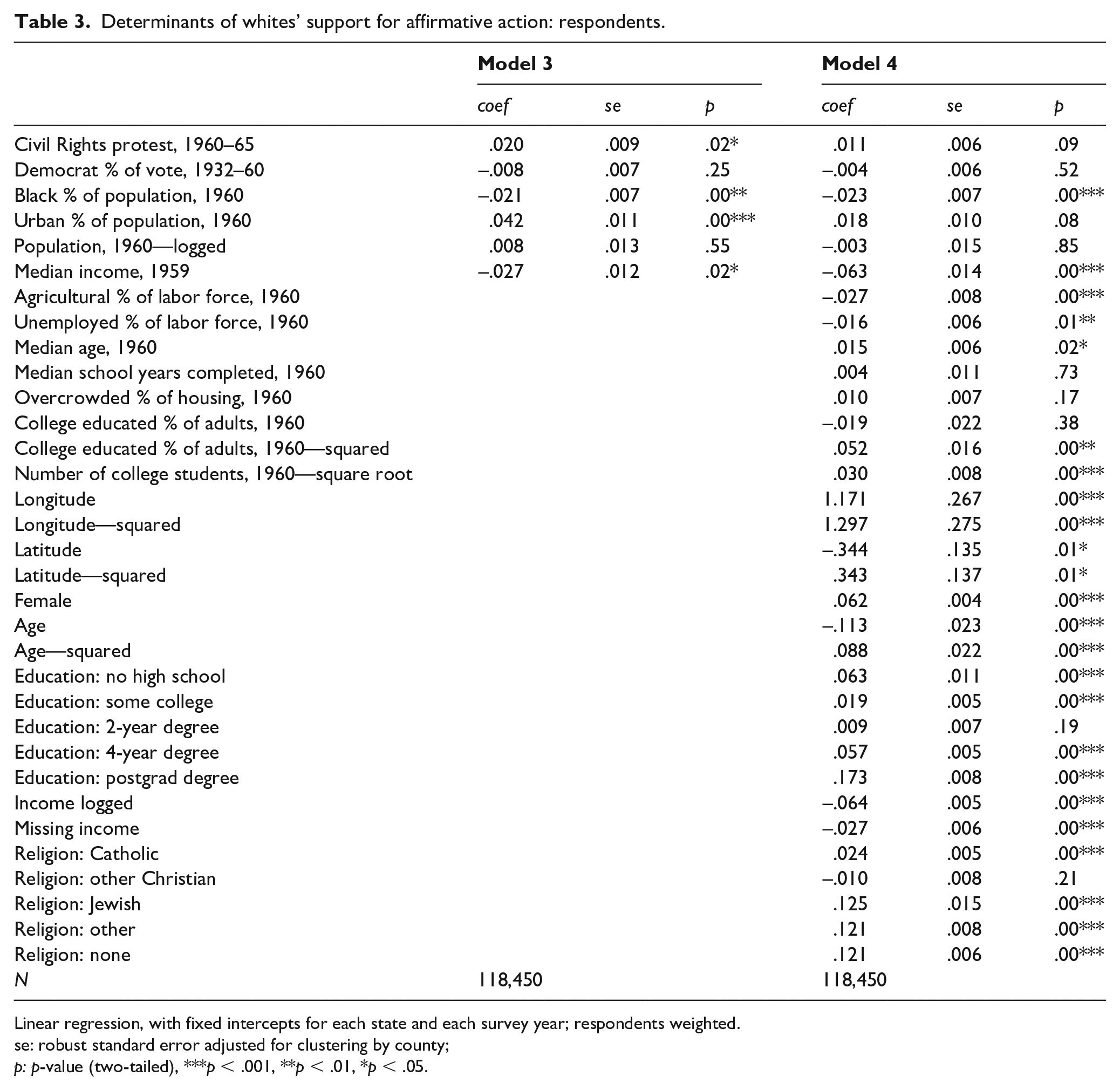
Linear regression, with fixed intercepts for each state and each survey year; respondents weighted.

se: robust standard error adjusted for clustering by county;

p: p-value (two-tailed), ***p < .001, **p < .01, *p < .05.

Model 4 adds county-level variables from Model 2 along with basic individual characteristics: sex, age, education, income, and religion (following Acharya et al., 2016—albeit substituting religion for religiosity). Women and younger people express greater support for affirmative action. Protestants (the reference category) are least likely to support affirmative action, while those with no religion or from non-Christian traditions are most likely. Support for affirmative action decreases with income. Education has a major effect, though it is not monotonic. People who only graduated from high school (the reference category) are least likely to support affirmative action. Those without a high school degree (7% of the total) are more likely to support affirmative action, as are those who attended a four-year college. For those with only a college degree, the probability of supporting affirmative action is higher by 6 percentage points; for those with a postgraduate degree, it is higher by 17. Even after adjusting for the individual’s education, the proportion of adults in the county with a college degree in 1960 has a strong effect. Figure 1 shows the average adjusted prediction, with the 95% confidence interval shaded; vertical lines indicate 10th, 50th, and 90th percentiles of the independent variable. Going from 5% to 15% increases the probability of support for affirmative action by 4 percentage points. The effect of college students in the county in 1960 is also strong. Going from 100 to 25,000 students increases the probability by 3 percentage points. The inclusion of the contextual and individual variables shrinks the effect of protest to 1 percentage point, and it is no longer statistically significant.

Figure 1.

Whites’ support for affirmative action, 2006–2011.

Table 4 summarizes the results using alternative measures of protest. Adding the variables in Model 4 reduces the effect of protest on support for affirmative action by at least two-thirds and the coefficients are no longer statistically significant. The table also shows results for the other outcome variables. (Supplemental Figures S2 and S3 depict the predicted effect of protest and our two key variables.) As before, the number of protest events has a statistically significant effect on racial resentment in Model 4, even though the effect’s magnitude is nearly halved. Out of nine combinations of three outcomes and three measures of protest, eight yield no statistically significant effect.

Table 4.

Summary of results: respondents.

Dependent variable	Protest variable	Model 3			Model 4			N
Dependent variable	Protest variable	coef	se	p	coef	se	p	N
Support for affirmative action	Binary	.018	.008	.02*	.011	.006	.09	118,450
Support for affirmative action	Event count—logged	.024	.008	.00**	.008	.007	.25	118,450
Support for affirmative action	Total participants—logged	.019	.008	.02*	.005	.007	.50	118,450
Racial resentment	Binary	−.017	.007	.01*	−.009	.006	.12	49,956
Racial resentment	Event count—logged	−.029	.006	.00***	−.017	.006	.01**	49,956
Racial resentment	Total participants—logged	−.021	.008	.00**	−.010	.007	.18	49,956
Identification with Democrats	Binary	.024	.010	.01	.015	.008	.06	118,375
Identification with Democrats	Event count—logged	.030	.010	.00	.013	.010	.18	118,375
Identification with Democrats	Total participants—logged	.026	.011	.02	.011	.010	.28	118,375

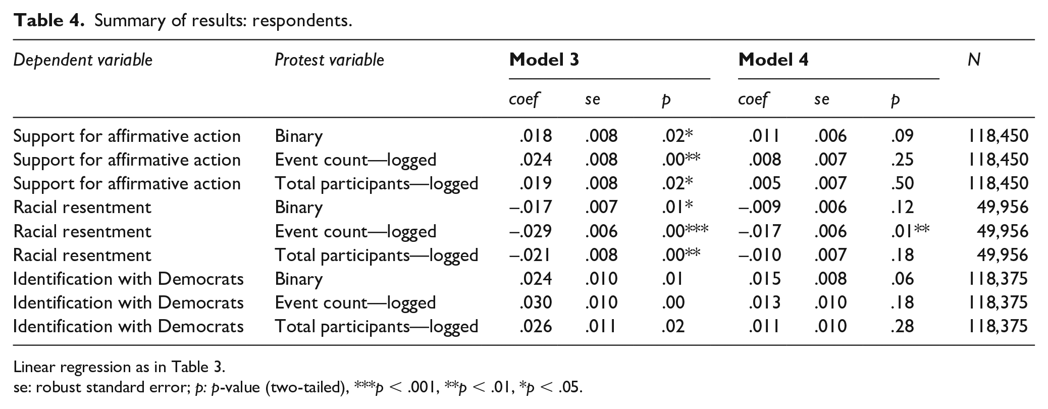
Linear regression as in Table 3.

se: robust standard error; p: p-value (two-tailed), ***p < .001, **p < .01, *p < .05.

Conclusion

According to Mazumder, whites who live in counties where Civil Rights protest occurred in the early 1960s—and was reported by the New York Times—are less likely to express racial resentment and more likely to support affirmative action and identify as Democrats. But Mazumder’s (2018: 932) “exhaustive set of observable historical confounders” excluded college education—one of the strongest predictors of protest and of racial attitudes. Once we incorporate education at the county level, along with basic contextual characteristics, protest has no statistically significant effect on support for affirmative action or on identification with the Democratic party. The number of protest events does have a statistically significant effect on racial resentment, but the occurrence of protest does not and neither does the total number of protesters. The evidence, in sum, is far weaker than Mazumder reports. Our additional socioeconomic variables do not exhaust the factors that predict variation in the incidence and magnitude of Civil Rights protest and that also shape whites’ attitudes on race.

Our reanalysis does not, of course, show that the Civil Rights movement of the 1960s failed to affect whites’ racial attitudes. Indeed, we share Mazumder’s intuition that the movement had a powerful influence, even given the longer-term decline in racist attitudes (Schuman et al., 1997). The problem is his assumption that the “intensity of the protest effect should be greater among areas more geographically proximate to the protest” (Mazumder, 2018: 927). This assumption makes sense in many historical contexts. High turnout in a city’s Tea Party rally, for example, mobilized right-wing activists who then affected local public opinion (Madestam et al., 2013). Sustained disruptive protest in Egypt after the 2011 revolution eroded support for democracy among people living in the vicinity (Ketchley and El-Reyyes, 2020). This assumption is much less appropriate for the Civil Rights movement, however.

In the South, protest actions were often not intended to persuade local whites to embrace racial equality. Many were intended to provoke violent repression that would shift public opinion hundreds of miles away, outside the South, and which would in turn force the Federal government to intervene (McAdam 1982). This strategy was used most famously by the Southern Christian Leadership Council in Birmingham and Selma, and it was deployed also in the Freedom Rides of 1962 and the Student Nonviolent Coordinating Committee’s projects in Mississippi and southwest Georgia. Therefore the assumption that the effect of protest would remain geographically circumscribed—after five decades had elapsed—is implausible. In the elaboration of explanatory mechanisms, causal inference and sustained historical inquiry should be treated as methodological complements (Kocher and Monteiro, 2016). For the nascent literature on attitudinal consequences of protest, leveraging qualitative case detail will be vital for understanding the channels through which protest makes an impact.

There are two broader implications of our analysis. The first is substantive. We find that the overall proportion of adults with a college degree in the county has a large impact on individual attitudes, after adjusting for the individual’s own level of education. This reinforces recent studies demonstrating similar contextual effects on attitudes to women and sexual minorities in England (Fielding, 2018) and on far-right voting in the Netherlands (Van Wijk et al., 2019). Whether such contextual effects are due to selective migration or to social influence remains an open question.

The second implication is methodological. Mazumder’s results are buttressed by a sensitivity test (Blackwell, 2014). It is deployed to argue for the implausibility of finding a confounding variable that could undermine the results; “such an unmeasured variable would have to explain more than twice the amount of variance in racial resentment than observed predictors such as urbanization, median income, and percent black” (Mazumder 2018: 929). In the equivalent of Model 1 for racial resentment, these five observed predictors together explain .006 of the variance. When added to this model, the square root of the number of college students explains .030 of the variance—five times more. Alternatively, adding the proportion of adults with college degrees (without the squared term) explains .051 of the variance—over eight times more.⁹ Indeed, this latter variable explains almost as much as all the state intercepts put together (.054). The lesson is that tests of statistical sensitivity cannot substitute for historical and theoretical understanding.

Supplemental Material

BiggsBarrieAndrews_LocalCivilRights_supplement – Supplemental material for Did local civil rights protest liberalize whites’ racial attitudes?

Supplemental material, BiggsBarrieAndrews_LocalCivilRights_supplement for Did local civil rights protest liberalize whites’ racial attitudes? by Michael Biggs, Christopher Barrie and Kenneth T. Andrews in Research & Politics

Footnotes

Acknowledgements

Particular thanks are due to Neal Caren, Neil Ketchley, Charles Rahal, and Brian Schaffner.

Declaration of conflicting interests

The author(s) declared no potential conflicts of interest with respect to the research, authorship, and/or publication of this article.

Funding

The author(s) disclosed receipt of the following financial support for the research, authorship, and/or publication of this article: Christopher Barrie was supported by a joint Nuffield/ESRC doctoral training studentship.

ORCID iD

Michael Biggs

Supplemental materials

The supplemental files are available at

The replication files are available at

Notes

Carnegie Corporation of New York Grant

This publication was made possible (in part) by a grant from the Carnegie Corporation of New York. The statements made and views expressed are solely the responsibility of the author.

References

Acharya

Blackwell

Sen

(2016) The political legacy of American slavery. Journal of Politics 78(3): 621–641.

Andrews

(1997) The impacts of social movements on the political process: The civil rights movement and Black electoral politics in Mississippi. American Sociological Review 62(5): 800–819.

Andrews

Beyerlein

Farnum

(2016) The legitimacy of protest: Explaining white Southerners’ attitudes toward the civil rights movement. Social Forces 94(3): 752–777.

Andrews

Biggs

(2006) The dynamics of protest diffusion: Movement organizations, social networks, and news media in the 1960 sit-ins. American Sociological Review 71(5): 752–777.

Beyerlein

Barwis

Crubaugh

Carnesecca

(2018) A new picture of protest: The national study of protest events. Sociological Methods and Research 47(3): 384–429.

Biggs

(2018) Size matters: Quantifying protest by counting participants. Sociological Methods and Research 47(3): 351–383.

Biggs

Andrews

(2015) Protest campaigns and movement success: Desegregating the U.S. South, 1960–61. American Sociological Review 80(2): 416–443.

Blackwell

(2014) A selection bias approach to sensitivity analysis for causal effects. Political Analysis 22(2):169–182.

Branton

Martinez-Ebers

Carey

Jr Matsubayashi

(2015) Social protest and policy attitudes: The case of the 2006 immigrant rallies. American Journal of Political Science 59(2): 390–440.

10.

Dalton

van Sickle

Weldon

(2009) The individual-institutional nexus of protest behaviour. British Journal of Political Science 40(1): 51-73.

11.

Fielding

(2018) The co-evolution of education and tolerance: Evidence from England. Social Forces 96(4): 1825–1850.

12.

Gelman

(2008) Scaling regression inputs by dividing by two standard deviations. Statistics in Medicine 27(15): 2865–2873.

13.

Harris

and Associates (1996) Racial Survey: Black Sample, Study No. 1634. Louis Harris Data Center Dataverse, University of North Carolina at Chapel Hill.

14.

Ketchley

El-Rayyes

(2020) Unpopular protest: Mass mobilization and attitudes to democracy in post-Mubarak Egypt. Journal of Politics forthcoming.

15.

Kocher

Monteiro

(2016) Lines of demarcation: Causation, design-based inference, and historical research. Perspectives on Politics 14(4): 952-975.

16.

Madestam

Shoag

Veuger

Yanagizawa-Drott

(2013) Do political protests matter? Evidence from the Tea Party movement. Quarterly Journal of Economics 128(4): 1633–1685.

17.

Mazumder

(2018) The persistent effect of U.S. civil rights protests on political attitudes. American Journal of Political Science 62(4): 922–935.

18.

McAdam

(1982) Political Process and the Development of Black Insurgency. Chicago: University of Chicago Press.

19.

McAdam

McCarthy

Olzak

Soule

(n.d.) Dynamics of Collective Action in the United States, 1960–1995. Available at: http://www.stanford.edu/group/collectiveaction/ (accessed 1 December 2019).

20.

McVeigh Cunningham

Farrell

(2014) Political polarization as a social movement outcome: 1960s Klan activism and its enduring impact on political realignment in southern counties, 1960 to 2000. American Sociological Review 79(6): 1144–1171.

21.

Motta

(2018) The polarizing effect of the March for Science on attitudes toward scientists. PS 51(4): 782–788.

22.

National Opinion Research Center (1973) General Social Survey. Available at: http://gss.norc.org/ (accessed 18 March 2019).

23.

Ortiz

Myers

Walls

Diaz

M-ED

(2005) Where do we stand with newspaper data? Mobilization 10(3): 397–419.

24.

Rosenbaum

(1984) The consequences of adjustment for a concomitant variable that has been affected by the treatment. Journal of the Royal Statistical Society Series A 147(5): 656–666.

25.

Rozenas

Zhukov

(2019) Mass repression and political loyalty: Evidence from Stalin’s ‘terror by hunger’. American Political Science Review 113(2): 569–583.

26.

Schuman

Steeh

Bobo

Krysan

(1997) Racial Attitudes in America: Trends and Interpretations, 2nd ed. Cambridge: Harvard University Press.

27.

Schussman

Soule

(2005) Process and protest: Accounting for individual participation. Social Forces 84(2): 1083–1108.

28.

Tertytchnaya

Lankina

(2020) Electoral protests and political attitudes under electoral authoritarianism. Journal of Politics 82(1): 285–299.

29.

Van Wijk

Bolt

Johnston

(2019) Contextual effects on populist radical right support: Consensual neighbourhood effects and the Dutch PVV. European Sociological Review 35(2): 225–238.

30.

Voigtländer

Voth

H-J

(2012) Persecution perpetuated: The medieval origins of anti-Semitic violence in Nazi Germany. Quarterly Journal of Economics 127(3):1339–1392.

31.

Wallace

Zepeda-Millán

Jones-Correa

(2014) Spatial and temporal proximity: Examining the effects of protests on political attitudes. American Journal of Political Science 58(2): 433–448.

32.

Young

Holsteen

(2017) Model uncertainty and robustness: A computational framework for multimodel analysis. Sociological Methods and Research 46(1): 3–40.

Supplementary Material

Please find the following supplemental material available below.

For Open Access articles published under a Creative Commons License, all supplemental material carries the same license as the article it is associated with.

For non-Open Access articles published, all supplemental material carries a non-exclusive license, and permission requests for re-use of supplemental material or any part of supplemental material shall be sent directly to the copyright owner as specified in the copyright notice associated with the article.

0.00 MB

0.70 MB