Sage Journals: Discover world-class research

Abstract

In recent years, research on the incumbency effect using a regression discontinuity design has flourished. Although the regression discontinuity design has allowed scholars to examine the incumbency effect in various electoral settings, previous studies have not measured what has traditionally been defined as the incumbency (dis)advantage. In this paper, I bring together methods from previous research, provide a consistent exposition thereof, and highlight some of the challenges of estimation and interpretation by applying these methods to election data from 10 different electoral settings.

Keywords

Incumbency effects regression discontinuity design elections

Introduction

In previous research, scholars have sought to overcome the methodological problems of measuring the effect of incumbency status on election outcomes (e.g., Ansolabehere, Snyder and Stewart, 2000; Erikson, 1971; Gelman and King, 1990; Lee, 2008; Levitt, 1994). However, the study of incumbency effects is complex because factors that affect incumbency status are also correlated with election outcomes. Regression discontinuity (RD) design offers a solution to some of the methodological problems associated with measuring the incumbency effect (Lee, 2008). If close elections are at least partly determined by chance, an RD design can be utilized to estimate the effect of winning an election on the outcome of the subsequent election.

Many recent studies have used RD design to estimate the incumbency effect in various electoral settings. The results of these studies are consistent with those of previous literature on the incumbency advantage in the United States (e.g., Ansolabehere and Snyder, 2002; Cox and Katz, 1996; Erikson, 1971; Gelman and King, 1990; Levitt and Wolfram, 1997), and report a similar size of incumbency advantage as that in the US (e.g., Lee, 2008; Erikson and Titiunik, 2015; Fowler, 2016). Outside of the US, researchers have also found an incumbency advantage in developed democracies (Ade, Freier and Odendahl, 2014; Eggers and Spirling, 2017; Hainmueller and Kern, 2008; Horiuchi and Leigh, 2009; Kendall and Rekkas, 2012; Redmond and Regan, 2015), while a growing body of literature has found no advantage or even a disadvantage of incumbency, particularly in developing democracies (Ariga, 2015; Ariga et al., 2016; Klašnja, 2015; Klašnja and Titiunik, 2017; Lee, 2016; Macdonald, 2014; Uppal, 2009).

Previous studies have adopted two approaches to measuring the incumbency effect using an RD design, the first of which is to estimate the incumbency effect at the party level (Ade, Freier and Odendahl, 2014; Ariga et al., 2016; Eggers and Spirling, 2017; Klašnja, 2015; Klašnja and Titiunik, 2017; Macdonald, 2014). Party-level RD analysis measures the effect of winning an election on a party’s vote share or probability of winning in the next election but to do so, it is necessary to define a “reference party.” In the US, for example, the Democratic or Republican parties could be used as such. The outcome variable is then defined as the Democratic (or Republican) share of the two-party vote or a dummy variable for the party’s victory. The running variable is defined as the Democratic (or Republican) share of the two-party vote in the previous election minus 0.5 (Lee, 2008). The treatment variable, winning an election, is defined as a dummy variable that takes the value 1 if the running variable exceeds 0.

In a multi-party system, the reference party is typically the most competitive party, which fields a large number of candidates across many elections: for example, the Liberal Democratic party in Japan (Ariga et al., 2016). Alternatively, a reference party can be defined as a “generic” incumbent party (Klašnja, 2015; Klašnja and Titiunik, 2017). For instance, Klašnja and Titiunik (2017) define an incumbent party for each municipality in Brazil as the party that wins an election at time t − 1. They measure the effect of winning an election at time t on the election outcome at time t + 1 for these incumbent parties.

However, the limitation of party-level analysis is that the RD design does not consider the possibility of a reference party being hurt by the incumbency status of other parties as much as it is helped by having an incumbent. In previous studies, the treatment variable has typically been coded as 1 if the reference party wins an election, and 0 otherwise. Therefore, the control group contains units in which a reference party faces an incumbent from other parties. As previous studies demonstrate (Erikson and Titiunik, 2015; Fowler and Hall, 2014), if almost all incumbents seek reelection and the incumbency status has, on average, the same effect for all parties, the party-level RD estimate would count the personal incumbency advantage twice. In contrast, in countries where only a small fraction of incumbents seek reelection, the RD estimate would underestimate the size of the personal incumbency (dis)advantage, because a large number of units in the treatment group contain open races.

The second approach is to analyze the incumbency effect at the candidate level (Ariga, 2015; De Magalhaes, 2015; Linden, 2004; Redmond and Regan, 2015; Uppal, 2009; Lee, 2016), one advantage of which is the applicability of this approach to countries with unstable party systems, where party switching is pervasive and/or candidates often run as independents. However, this approach can be problematic as we cannot observe the outcome for candidates who do not run in the next election. While some studies simply exclude such candidates from the sample (e.g., Uppal, 2009; Lee, 2016), doing so would result in a biased estimate if candidates’ retirement decisions are affected by their incumbency status and the expected outcome of the future election.

One potential solution to this issue is to measure the effect of winning an election on the probability of winning the subsequent election unconditional on running (Ariga et al., 2016; De Magalhaes, 2015; Redmond and Regan, 2015). In other words, the outcome variable is defined as a dummy variable that takes the value “1” if a candidate runs in and wins the next election, and “0” otherwise. However, this analysis is problematic in treating all candidates who do not rerun as losers. Therefore, the unconditional RD estimand does not inform us whether the estimated effect is, in fact, caused by a candidate’s incumbency status or simply because incumbents are more (or less) likely to rerun than losers.

In this paper, I bring together methods from previous applied papers in economics and political science, provide a consistent exposition thereof, and highlight some of the challenges of estimation and interpretation by applying these methods to election data from 10 different electoral settings.¹ First, for the party-level analysis, I discuss how to measure the personal incumbency effect using winning a close election as an instrument for incumbency status. Second, to address the sample selection issue of the candidate-level RD design, following Lee (2009) and Anagol and Fujiwara (2016), I estimate bounds on the average treatment effect of winning, conditional on running in an election. The results suggest that the estimated effects of incumbency critically depend on how the dependent variable is defined. Since the RD design estimates the effect of winning an election on the outcome of the subsequent election, it is important to treat candidates’ rerunning decisions carefully.

Party-level analysis

I first discuss how to measure the incumbency effect at the party level by formulating the problem in the potential outcome framework, also called the Rubin Causal Model (e.g., Imbens and Rubin 2015). Let W_d be a dummy variable indicating whether a reference party won in district d at time t. Let VM_d be the running variable, the vote margin of the reference party in district d at time t. Since the RD design estimates the effect of winning a close election, all results are conditional on VM_d = 0. For simplicity, I suppress this condition.

The treatment of interest, denoted by I_d, is defined as the reference party’s incumbency status in district d at time t + 1, which is “1” if an incumbent from the reference party runs at t − 1, if the incumbent running at t + 1 is from another party, and “0” otherwise. The reference party (or non-reference party) will be assigned to treatment if it wins an election at time t. However, it will receive treatment—that is, have an incumbent running in the election at time t + 1—only if the incumbent runs again. Following the Rubin Causal Model’s convention, I will call incumbents who run at t + 1 compliers (C) and those who do not noncompliers (N). Note that the incumbency status I_d depends on the election outcome at time t, W_d. If all winners at time t run at t + 1, we would have I_d = 2W_d – 1. In other words, if the reference party wins at time t + 1, its incumbent will run at time t + 1, and if it loses it will face an incumbent from another party. Otherwise, in some districts where a reference party has won (lost) at t, I_d can take a value of 1 (–1) or 0, depending on whether or not the incumbent decides to rerun.

Previous studies (e.g., Lee 2008) have focused on the effect of winning an election on the election outcome at t + 1, rather than the effect of having an incumbent in the election. If the usual assumptions of RD design are valid, the intention-to-treat (ITT) analysis can estimate the causal relationship between winning an election at t and the election outcome at t + 1.² However, as Fowler and Hall (2014) notes, the ITT analysis can estimate neither the personal nor the partisan incumbency effect.

To see this, let I_d(0) and I_d(1) denote the potential treatment a district would receive if assigned to W_d = 0 and W_d = 1, respectively. For each district, we can only observe one of the two potential treatments, I_d = W_dI_d(1) + (1 − W_d)I_d(0). Since the incumbent party may not field a candidate in an election, there are four possible values of (I_d(1), I_d(0)): (1,−1), (1,0), (0,−1), and (0,0).³ I assume that noncompliance is one-sided: A party that lost at time t cannot have an incumbent at t + 1. I relax this assumption in Online Appendix C. We can classify each unit into one of the four groups based on the potential treatment:

G_{d} = {\begin{array}{l} C C, & if (I_{d} (1), I_{d} (0)) = (1, - 1) \\ C N, & if (I_{d} (1), I_{d} (0)) = (1, 0) \\ N C, & if (I_{d} (1), I_{d} (0)) = (0, - 1) \\ N N, & if (I_{d} (1), I_{d} (0)) = (0, 0) \end{array}

(1)

Let Y_d be the outcome of interest. The realized outcome, Y_d(W_d,I_d(W_d)), which depends on I_d as well as W_d, can take one of the following four values: $Y_{d} (1, 1), Y_{d} (1, 0), Y_{d} (0, - 1) and Y_{d} (0, 0)$ .

We can write the ITT effect as

\begin{array}{l} I T T = E [Y_{d} (1, I_{d} (1)) - Y_{d} (0, I_{d} (0))] \\ = E [Y_{d} (1, 1) - Y_{d} (0, - 1) | G_{d} = C C] \cdot Prob (G_{d} = C C) \\ + E [Y_{d} (1, 1) - Y_{d} (0, 0) | G_{d} = C N] \cdot Prob (G_{d} = C N) \\ + E [Y_{d} (1, 0) - Y_{d} (0, - 1) | G_{d} = N C] \cdot Prob (G_{d} = N C) \\ + E [Y_{d} (1, 0) - Y_{d} (0, 0) | G_{d} = N N] \cdot Prob (G_{d} = N N) . \end{array}

(2)

Under certain assumptions, we can use the assignment, W_d, as our instrument for the treatment, I_d, and estimate the causal effect of personal incumbency on the election outcome using a fuzzy RD design (see also Fowler, 2016). To do so, we must first assume that the effect of incumbency is the same for the reference party and other parties.

Assumption 1a. The effect of incumbency, denoted by θ, is the same for all parties

\begin{array}{l} E [Y_{d} (1, 1) - Y_{d} (0, - 1) | G_{d} = C C] = 2 θ \\ and \\ E [Y_{d} (1, 1) - Y_{d} (0, 0) | G_{d} = C N] = E [Y_{d} (1, 0) - Y_{d} (0, - 1) | G_{d} = N C] = θ \end{array}

In other words, the reference party is hurt by the incumbency status of other parties as much as it is helped by having its own incumbent running. This assumption is routinely made in the literature on the incumbency advantage in the USA (e.g., Ansolabehere and Snyder, 2002; Erikson and Titiunik, 2015; Levitt and Wolfram, 1997). It is plausible in countries like the USA, which has a stable two-party system, but the incumbency status may have heterogeneous effects for different parties in other countries. For instance, if incumbents have advantages over other candidates because of what they can do for their constituents in office, incumbents from minor parties may have a smaller advantage because their ability to do what their constituents want is limited. To estimate the personal incumbency effect using a fuzzy RD design, the following additional assumption must be made regarding G_d = NN.

Assumption 1b. For all d with G_d = NN, either Y_d(1,0) = Y_d(0,0) or Prob(G_d = NN) = 0

Assumption 1b states that either (a) in districts where no incumbent would run, winning itself has no effect on the election outcome or (b) the proportion of districts where no incumbent from any party would run is negligible. Note that the second part of this assumption does not imply that there will be no open race, because G_d denotes latent groups. The first part of the assumption, which has been characterized in previous literature (e.g., Erikson and Titiunik, 2015; Fowler, 2016) as a no “partisan” incumbency effect assumption, comprises an exclusion restriction because it rules out a direct effect of assignment on the election outcome. This is a key identifying assumption for a fuzzy RD design. It should be noted that assumption 1a implicitly presupposes that the partisan incumbency effect is also negligible for other latent groups, because party incumbency changes whenever the reference party wins or loses.

The exclusion restriction is a strong assumption and its applicability should be carefully examined in different electoral settings. Previous studies on US elections demonstrate that the advantage of having a retiring incumbent is negligible (Broockman, 2009; Butler and Butler, 2006; Fowler, 2016), thus suggesting no partisan incumbency advantage. However, the partisan incumbency effect may be non-zero in other electoral contexts. Kendall and Rekkas (2012) suggest that the partisan incumbency has a zero or negative effect in the Canadian parliamentary elections. In Brazilian mayoral elections, parties are hurt by having a term-limited incumbent (Klašnja and Titiunik, 2017), suggesting a “partisan incumbency disadvantage.” Similarly, Fowler and Hall (2014) suggest that the partisan incumbency effect can be negative in term-limited contexts, while Eggers (2017) provides a theoretical reason for the partisan incumbency disadvantage in the presence of term limits. If we allow the existence of a partisan incumbency effect, an RD design alone, fuzzy or sharp, cannot provide an unbiased estimate for either a partisan or a personal incumbency effect. See Online Appendix D for details.

If assumptions 1a and 1b hold, the incumbency effect consists entirely of a personal incumbency effect. However, the ITT estimate would almost always either exaggerate or depreciate the personal incumbency effect. To observe this, we can rewrite the ITT effect as

\begin{array}{l} I T T = 2 θ \cdot Prob (G_{d} = C C) + θ \cdot Prob (G_{d} = C N) + θ \cdot Prob (G_{d} = N C) \\ = θ \cdot [Prob (G_{d} = C C) + Prob (G_{d} = C N)] + θ \cdot [Prob (G_{d} = C C) + Prob (G_{d} = N C)] \\ = θ \cdot [Prob (I_{d} (1) = 1) + Prob (I_{d} (0) = - 1)] = θ μ \end{array}

(3)

where $μ = Prob (I_{d} (1) = 1) + Prob (I_{d} (0) = - 1)$ . The personal incumbency effect, θ, can be estimated using a fuzzy RD design because we can estimate both the ITT effect and µ. This equation demonstrates that the ITT estimate for θ would be unbiased under the razor-thin condition that $Prob (I_{d} (1) = 1) + Prob (I_{d} (0) = - 1) = 1$ : that is, on average, exactly half of the incumbents rerun. If, on average, more than 50 percent of incumbents rerun, the ITT would overestimate the magnitude of θ, whereas it would underestimate the magnitude of θ if fewer than half of incumbents run at t + 1.⁴

In the remaining section, I demonstrate how the fuzzy RD estimates for incumbency effects can diverge from the ITT estimate. Table 1 presents the percentage of districts where the winners of time t run again at time t + 1. The first two columns show the percentages for the full sample, while the remaining two columns show the percentages for the RD sample. The return rate of incumbents is the highest in the US House elections, where more than 80 percent of incumbents seek reelection. In contrast, in Indian Lok Sabha elections (national parliamentary elections), fewer than 40 percent of winners at time t reran at time t + 1. Figure 1 shows the RD estimate of µ in equation (3).⁵

Table 1.

Percent of constituents where incumbents run for reelection.

	Full sample	N	RD sample	N
	Incumbent runs at t + 1 (%)		Incumbent runs at t + 1 (%)
USA, House
Reference party won at t	87.0	12,758	83.8	2,051
Reference party lost at t	85.4	10,639	83.9	2,154
Japan, House
Reference party won at t	83.8	895	81.4	404
Reference party lost at t	70.0	753	71.6	380
Romania, Mayor
Reference party won at t	91.1	4,235	86.5	654
Reference party lost at t	51.7	2,581	70.2	581
Canada, House
Reference party won at t	63.6	3,769	59.4	1,769
Reference party lost at t	69.9	3,710	66.0	1,603
UK, House
Reference party won at t	62.0	7,194	59.1	1,969
Reference party lost at t	63.7	6,082	58.8	1,703
Korea, National Assembly
Reference party won at t	53.3	676	54.9	235
Reference party lost at t	54.7	704	51.5	274
India, House
Reference party won at t	36.4	2,065	36.2	882
Reference party lost at t	39.8	2,092	36.0	847

Figure 1.

Effect of winning an election on the incumbency status of the reference party.

Figure 2 presents the estimated effects of incumbency on election outcomes. The dependent variable for Figure 2(a) is a dummy variable indicating whether the reference party wins at time t + 1. In Figure 2(b), the dependent variable is the reference party’s vote margin divided by 2. The ITT estimates demonstrate that winning an election has a positive effect on the outcome of the next election in the US, Canada, and the United Kingdom, consistent with previous studies (e.g., Ansolabehere and Snyder, 2002; Eggers and Spirling, 2017; Kendall and Rekkas, 2012). The fuzzy RD estimate diverges substantially from the ITT estimate in the US House elections: the fuzzy RD estimate is approximately 10 percent smaller than the ITT estimate. The difference, however, is much smaller in Canadian and UK elections, because the first stage RD estimates are close to 1 (1.125 and 1.132 for Canada and the UK, respectively). As equation (3) demonstrates, the two estimates will be similar if µ is close to 1.

Figure 2.

RD estimates of the incumbency effect (party-level analysis).

In contrast, where the ITT estimate is negative, the first stage RD estimate tends to be smaller than 1, leading to the underestimation of the size of the personal incumbency effect. As shown in Figure 2, the estimated effects of incumbency on the probability of winning and the vote margin are negative in South Korea and India. The estimates are statistically significant, except in the Indian Lok Sabha when a dummy for winning is used as a dependent variable, in which case the estimate is only marginally significant. In all of these elections, the size of the ITT estimate is smaller than the size of the fuzzy RD estimate, although the difference is not as great as in the US House elections.

Finally, the ITT estimate is not statistically different from 0 in Japanese House elections and Romanian mayoral elections.⁶ The results suggest that the incumbency effects in these countries are likely to be zero unless the partisan and personal incumbency effects have different signs. If the incumbency effects, personal and partisan, are 0, the fuzzy RD estimate would not differ from the ITT estimate, because both are zero.

To summarize, the analyses in this section demonstrate that the fuzzy RD estimate diverges from the ITT estimate if (a) the incumbency effect is not 0 and (b) the estimated effect of winning on µ is close to 0 or 2. Among the cases analyzed in this section, the US House elections and, to a lesser extent, the South Korean and Indian legislative elections, fit these two criteria. If the exclusion restriction assumption holds, a sharp RD design would lead to over- or underestimation of the personal incumbency effect. Moreover, the ITT analysis tends to underestimate the size of the incumbency disadvantage because fewer than half of the incumbents seek reelection; however, more data are required to ascertain whether this pattern can be generalized to countries where incumbency has a negative effect on election outcomes.

Candidate-level analysis

I now turn to the candidate-level analysis. As previously mentioned, the unconditional RD analysis measures the effect of winning an election on electoral success in the subsequent election, treating all candidates who do not rerun as losers. Therefore, it does not tell us whether the effect is driven by the incumbency or by the fact that losing candidates find it more difficult to rerun. Unless all winners and runners-up of close elections decide to rerun, or the candidacy is unrelated to the future election outcome, the unconditional RD estimate would differ from the conditional RD estimate, which measures the effect of candidates’ incumbency status on election outcomes.

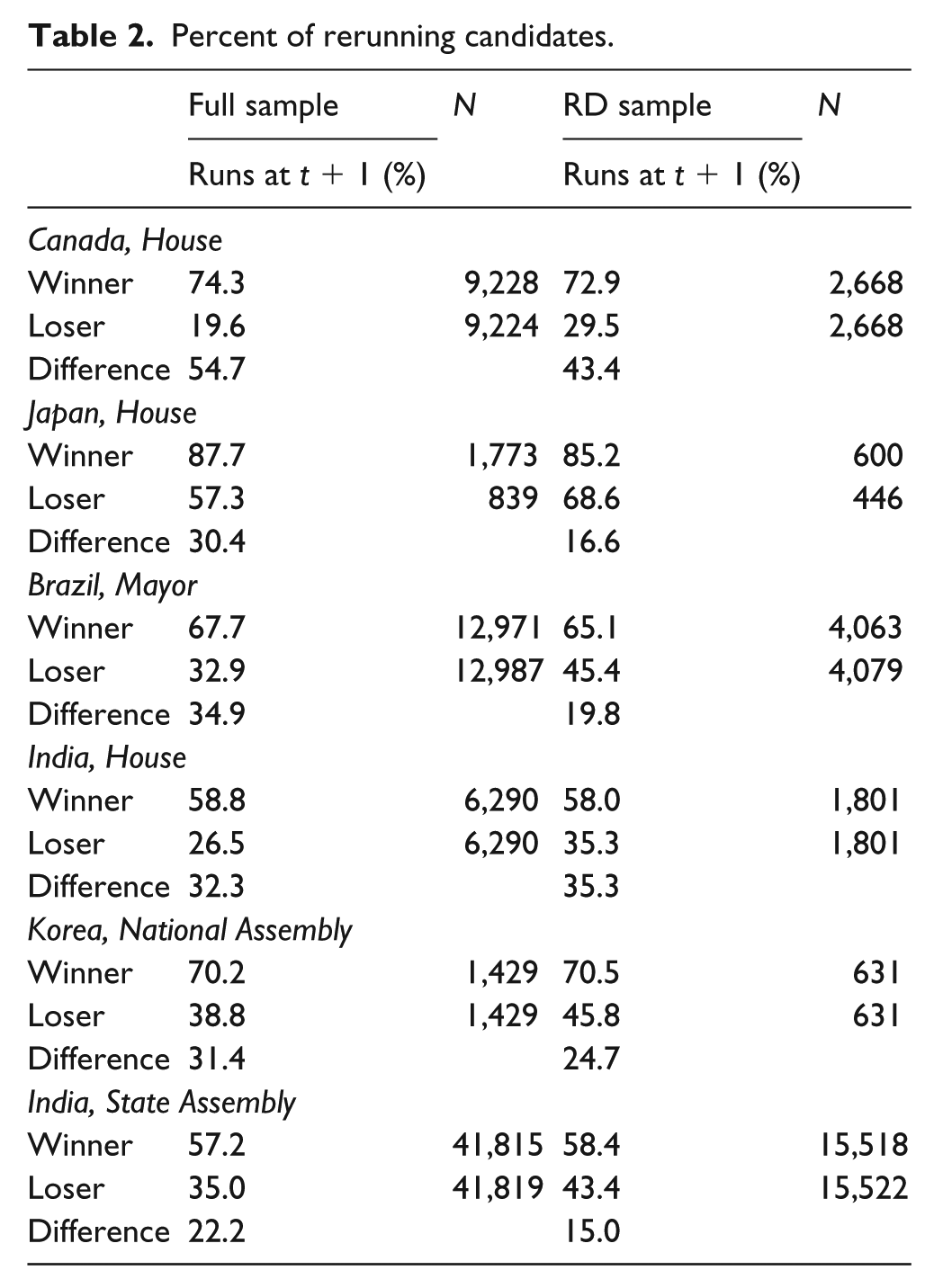
Table 2 presents the percentage of candidates rerunning in the next election.⁷ As shown in the table, winners are more likely than losers to run in the subsequent election.⁸ For instance, in Canada, a developed Western democracy, incumbents are 2.5–3.7 times more likely than runners-up to rerun in the next election. The difference in rerunning rate between incumbents and losers tends to be smaller in developing democracies, but winners are approximately 15–30 percent more likely to rerun.

Table 2.

Percent of rerunning candidates.

	Full sample	N	RD sample	N
	Runs at t + 1 (%)		Runs at t + 1 (%)
Canada, House
Winner	74.3	9,228	72.9	2,668
Loser	19.6	9,224	29.5	2,668
Difference	54.7		43.4
Japan, House
Winner	87.7	1,773	85.2	600
Loser	57.3	839	68.6	446
Difference	30.4		16.6
Brazil, Mayor
Winner	67.7	12,971	65.1	4,063
Loser	32.9	12,987	45.4	4,079
Difference	34.9		19.8
India, House
Winner	58.8	6,290	58.0	1,801
Loser	26.5	6,290	35.3	1,801
Difference	32.3		35.3
Korea, National Assembly
Winner	70.2	1,429	70.5	631
Loser	38.8	1,429	45.8	631
Difference	31.4		24.7
India, State Assembly
Winner	57.2	41,815	58.4	15,518
Loser	35.0	41,819	43.4	15,522
Difference	22.2		15.0

Although it is straightforward to estimate the unconditional RD estimate, estimating the conditional effect of winning is more complicated, because candidates’ decisions to rerun are affected by incumbency status, as well as by the prospect of future election. Furthermore, the candidate’s performance in the next election (i.e., how the candidate would do if he or she ran) is not observed. Following Lee (2009) and Anagol and Fujiwara (2016), I estimate bounds on the effect of winning an election on the probability of winning the next election conditional on running.⁹ Let W_i be a dummy variable for our treatment, indicating whether candidate i won an election at time t. For each unit, let R_i(0) and R_i(1) be the potential outcome variables, indicating whether a candidate runs at time t + 1 when W_i = 0 and W_i = 1, respectively. Similarly, let Y_i(0) and Y_i(1) be our potential outcome variables. We can only observe $Y_{i} = R_{i} [W_{i} Y_{i} (1) + (1 - W_{i}) Y_{i} (0)]$ , where $R_{i} = W_{i} R_{i} (1) + (1 - W_{i}) R_{i} (0)$ . In other words, Y_i is observable only when R_i = 1; that is, when a candidate decides to rerun at time t + 1. Note also that we can only observe one of the two potential outcomes of R_i, R_i(0), and R_i(1), which depend on the election outcome at time t.

Let VM_i be the vote margin of candidate i at time t, the running variable. The unconditional RD analysis estimates $E [Y_{i} (1) R_{i} (1) - Y_{i} (0) R_{i} (0) | V M_{i} = 0]$ , whereas the conditional RD effect is $E [Y_{i} (1) - Y_{i} (0) | V M_{i} = 0, R_{i} = 1]$ .¹⁰

To estimate the bounds, I first classify each candidate into one of the following four latent groups (G_i): “always-takers (AT),” those who always run; “never-takers (NT),” those who never run; “compliers (CO),” those who run only if they have won the previous election; and “defiers (DF),” those who run only if they have lost the previous election. I assume that there are no defiers: if a candidate who lost an election decides to rerun, she would also rerun had she won the election.

Assumption 3a. There are no defiers: R_i(1) ⩾ R_i(0) for all i.

Under this assumption, we can write the conditional effect of winning, the incumbency (dis)advantage, as follows (for simplicity, I suppress the conditioning on VM_i = 0)

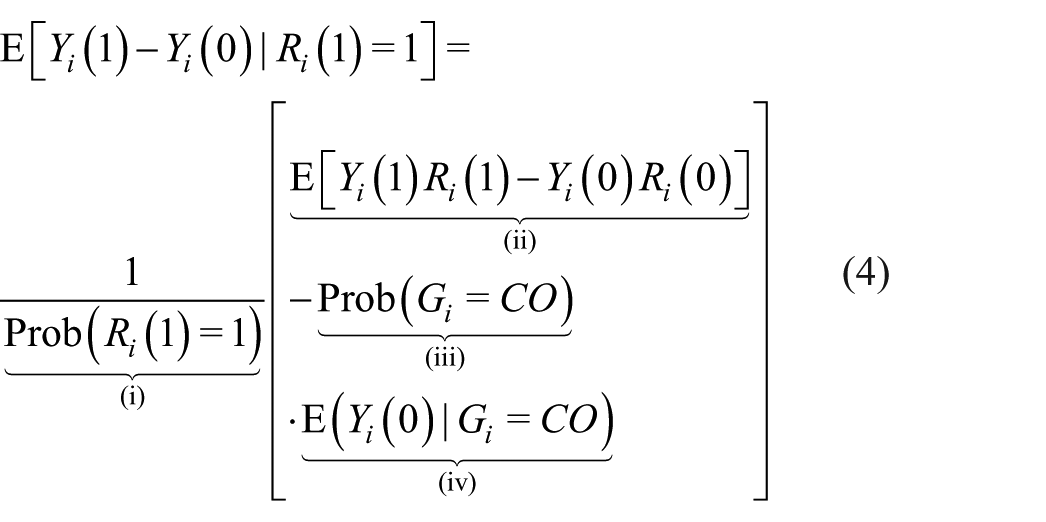
\begin{array}{l} E [Y_{i} (1) - Y_{i} (0) | R_{i} (1) = 1] = \\ \frac{1}{\underset{(i)}{\underset{︸}{Prob (R_{i} (1) = 1)}}} [\underset{(ii)}{\underset{︸}{E [Y_{i} (1) R_{i} (1) - Y_{i} (0) R_{i} (0)]}} - \underset{(iii)}{\underset{︸}{Prob (G_{i} = C O)}} \cdot \underset{(iv)}{\underset{︸}{E (Y_{i} (0) | G_{i} = C O)}}] \end{array}

(4)

where (i) is $\lim_{m ↓ 0} E [R_{i} | V M_{i} = m]$ ; (ii) is the unconditional RD effect on Y_i; (iii) is the RD effect on R_i; and (iv) is the probability that a complier who lost at time t would win at time t + 1. The proof is presented in Online Appendix E. Since a complier would run at time t + 1 only if she had won the previous election, R_i(0) = 0 for G_i = CO; therefore, (iv) is unobservable.

We can obtain the upper bound by assuming $E [Y_{i} (0) | G_{i} = C O] = 0$ ; that is, a complier who lost at time t would never win at time t + 1. The lower bound can be obtained by plugging in the largest possible value of (iv), which is 1. However, following Anagol and Fujiwara (2016), I assume that the probability that a complier who barely lost at time t would win at time t + 1 had she chosen to run is less than or equal to the probability that a winner of a close election who reran at time t + 1 would win that year. More formally, I assume the following:

Assumption 3b.

E [Y_{i} (0) | G_{i} = C O] \leq E [Y_{i} (1) | G_{i} = C O or G_{i} = A T]

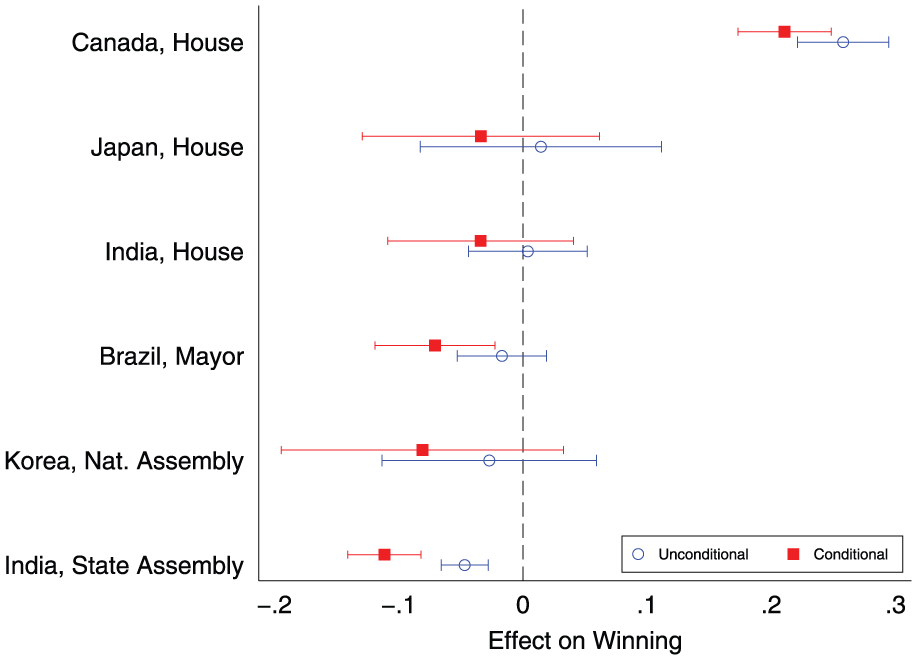
Figure 3 presents the results.¹¹ The RD estimate of the unconditional effect of winning is positive and statistically significant for Canada but negative in all other countries, although the negative effect is statistically significant only for Indian State Assembly elections. Interestingly, in countries where the unconditional RD estimate is not positive, it is outside, or very close to, the upper bound. As Figure 3 shows, the estimates are located on the right side of the bounds except for Canada. Note that the upper bound is calculated under the very restrictive assumption that a complier who lost at time t would never win the next election had she chosen to run. Therefore, the conditional RD effect of winning is likely to be strictly smaller than the upper bound. Note also that the estimates for the lower bound are negative and statistically significant in Brazil, India, and Korea, suggesting that the unconditional estimate is likely to underestimate the size of the incumbency effect in these countries.

Figure 3.

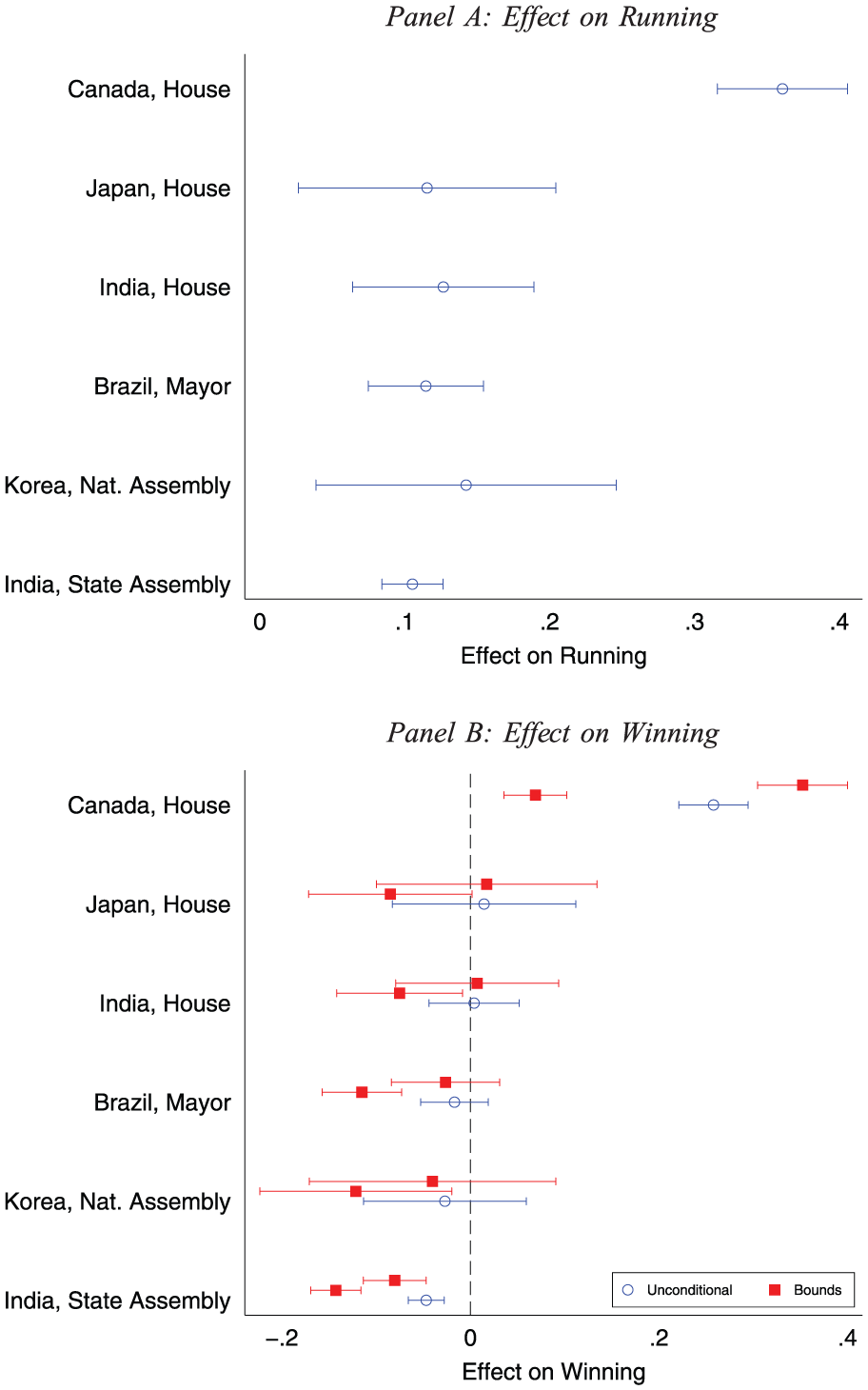
Conditional/unconditional effect of winning (candidate-level analysis).

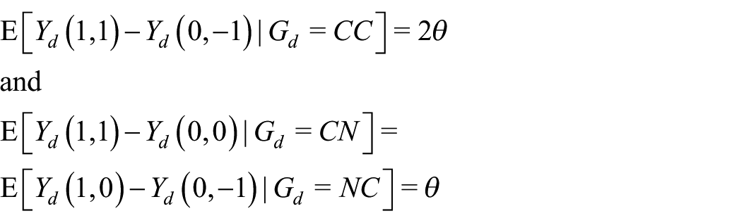
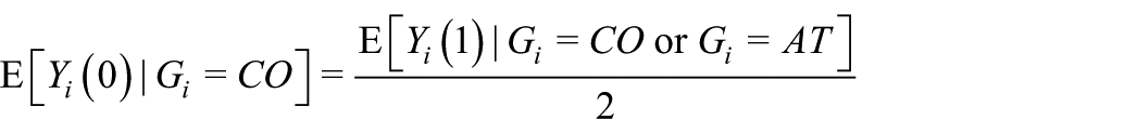
In Figure 4, I repeat the analysis of (b) in Figure 3, assuming that the probability that a complier who lost at time t would win at time t + 1 is only one-half the probability that an incumbent who reran would win at time t + 1, i.e.,

Figure 4.

RD estimates of the incumbency effect (candidate-level analysis).

Assumption 3c.

E [Y_{i} (0) | G_{i} = C O] = \frac{E [Y_{i} (1) | G_{i} = C O or G_{i} = A T]}{2}

As expected, the figure shows that the unconditional RD estimate exceeds the conditional RD estimate. To ascertain why the unconditional RD will underestimate the size of the incumbency disadvantage, let θ denote $E [Y_{i} (1) - Y_{i} (0) | R_{i} (1) = 1]$ , the personal incumbency effect, and τ denote $E [Y_{i} (1) R_{i} (1) - Y_{i} (0) R_{i} (0)]$ , the unconditional effect of winning. Then, from equation (4), we obtain $τ = θ \cdot Prob (R_{i} (1) = 1) + Prob (G_{i} = C O) \cdot E (Y_{i} (0) | G_{i} = C O)$ . Suppose that θ < 0. Unless not all winners run in the next election, Prob(R_i(1) = 1) < 1,¹² τ will underestimate the magnitude of θ. Furthermore, the final term on the right side of the equation is greater than or equal to zero, pushing τ further toward zero.

To summarize, the results suggest that the unconditional RD analysis may lead to overestimation of the incumbency advantage and underestimation of the size of the incumbency disadvantage. However, it should be noted that while we can estimate the bounds on the conditional incumbency effect, they may fail to provide conclusive evidence of an incumbency effect. Among the cases analyzed in this section, in three of four elections where the estimates for the lower bound were negative and statistically significant, the estimates for the upper bound failed to reach statistical significance.

Conclusion

In this paper, I have discussed how one can (or cannot) estimate the incumbency effect using an RD design. At the party level, I demonstrated that, based on some assumptions, we can recover the personal incumbency effect using a fuzzy RD design. At the candidate level, following Anagol and Fujiwara (2016) and Lee (2009), I provided bounds on the conditional effect of winning, the personal incumbency effect. The results suggest that it is important to recognize what RD analysis can and cannot estimate. As some recent studies suggest (Erikson and Titiunik, 2015; Fowler and Hall, 2014; Sekhon and Titiunik, 2012), a quasi- or natural experimental design like an RD design does not always recover the quantity that is of theoretical interest. Furthermore, the validity of an RD design to estimate the incumbency effect relies on some key assumptions that should be carefully examined in each electoral setting.

It should be emphasized, however, that I do not claim that the previous RD estimates are of little theoretical importance. They tell us that winning parties or candidates tend to win or lose in the next election, which may be due to what incumbents do in office (e.g., constituency service or rent-seeking in the case of incumbency disadvantage) or parties’ candidate nomination processes that affect whether incumbents can easily seek reelection. For instance, suppose that major parties in a country are very successful at weeding out unpopular incumbents. It would then be plausible that the party-level RD analysis may find a zero or positive effect of winning even when there is, on average, a personal incumbency disadvantage. In contrast, it is also possible that parties in a country tend to nominate incumbents who are loyal to the parties’ bosses but not to the voters. In this case, we may find that winning has an adverse effect on parties when, in fact, these incumbents would enjoy a personal electoral advantage if allowed to run. Therefore, studying whether/how the personal incumbency effect diverges from the previous RD estimates would allow us to better understand the sources of incumbency (dis)advantage and shed light on the electoral politics of developed and developing democracies.

Supplemental Material

online_appendix_RAP – Supplemental material for Estimating Incumbency Effects Using Regression Discontinuity Design

Supplemental material, online_appendix_RAP for Estimating Incumbency Effects Using Regression Discontinuity Design by B. K. Song in Research & Politics

Footnotes

Acknowledgements

I thank the anonymous reviewers and the associate editor Andy Eggers for their helpful comments and constructive suggestions.

Declaration of conflicting interest

The authors declare that there is no conflict of interest.

Funding

This research received no specific grant from any funding agency in the public, commercial, or not-for-profit sectors.

ORCID iD

BK Song .

Supplemental materials

The supplemental files are available at .

The replication files are available at https://dataverse.harvard.edu/dataset.xhtml?persistentId=doi:10.7910/DVN/JSOWUR&version=DRAFT.

Notes

Carnegie Corporation of New York Grant

This publication was made possible (in part) by a grant from the Carnegie Corporation of New York. The statements made and views expressed are solely the responsibility of the author.

References

Ade

Freier

Odendahl

(2014) Incumbency effects in government and opposition: Evidence from Germany. European Journal of Political Economy 36: 117–134.

Anagol

Fujiwara

(2016) The runner-up effect. Journal of Political Economy 124(4): 927–991.

Ansolabehere

Snyder

Jr (2002) The incumbency advantage in US elections: An analysis of State and Federal offices, 1942–2000. Election Law Journal 1(3): 315–338.

Ansolabehere

Snyder

Jr Stewart

(2000) Old voters, new voters, and the personal vote: Using redistricting to measure the incumbency advantage. American Journal of Political Science 44(1): 17–34.

Ariga

(2015) Incumbency disadvantage under electoral rules with intraparty competition: Evidence from Japan. Journal of Politics 77(3): 874–887.

Ariga

Horiuchi

Mansilla

and Umeda Michio (2016) No sorting, no advantage: Regression discontinuity estimates of incumbency advantage in Japan. Electoral Studies 43: 21–31.

Broockman

D E

(2009) Do congressional candidates have reverse coattails? Evidence from a regression discontinuity design. Political Analysis 17(4): 418–434.

Butler

(2006) Splitting the difference? Causal inference and theories of split-party delegations. Political Analysis 14(4): 439–455.

Calonico

Cattaneo

Titiunik

(2014) Robust nonparametric confidence intervals for regression-discontinuity designs. Econometrica 82(6): 2295–2326.

10.

Cox

Katz

(1996) Why did the incumbency advantage in U.S. House elections grow? American Journal of Political Science 40(2): 478–497.

11.

De Magalhaes

(2015) Incumbency effects in a comparative perspective: Evidence from Brazilian mayoral elections. Political Analysis 23(1): 113–126.

12.

Eggers

(2017) Quality-based explanations of incumbency effects. Journal of Politics 79(4): 1315–1328.

13.

Eggers

Fowler

Hainmueller

Hall

Snyder

Jr (2015) On the validity of the regression discontinuity design for estimating electoral effects: New evidence from over 40,000 close races. American Journal of Political Science 59(1): 259–274.

14.

Eggers

Spirling

(2014) Electoral security as a determinant of legislator activity, 1832–1918: New data and methods for analyzing British political development. Legislative Studies Quarterly 39(4): 593–620.

15.

Eggers

Spirling

(2017) Incumbency effects and the strength of party preferences: Evidence from multiparty elections in the United Kingdom. Journal of Politics 79(3): 903–920.

16.

Erikson

(1971) The advantage of incumbency in Congressional elections. Polity 3(3): 395–405.

17.

Erikson

Titiunik

(2015) Using regression discontinuity to uncover the personal incumbency advantage. Quarterly Journal of Political Science 10(1): 101–119.

18.

Fowler

(2016) What explains incumbent success? Disentangling selection on party, selection on candidate characteristics, and office-holding benefits. Quarterly Journal of Political Science 11(3): 313–338.

19.

Fowler

Hall

(2014) Disentangling the personal and partisan incumbency advantages: Evidence from close elections and term limits. Quarterly Journal of Political Science 9(4): 501–531.

20.

Gelman

King

(1990) Estimating incumbency advantage without bias. American Journal of Political Science 34(4): 1142–1164.

21.

Hainmueller

Kern

(2008) Incumbency as a source of spillover effects in mixed electoral systems: Evidence from a regression-discontinuity design. Electoral Studies 27(2): 213–227.

22.

Horiuchi

Leigh

(2009) Estimating incumbency advantage: Evidence from multiple natural experiments. Working Paper.

23.

Imbens

Rubin

(2015) Causal Inference in Statistics, Social, and Biomedical Sciences. Cambridge University Press. Available at http://wwwdocs.fce.unsw.edu.au/economics/news/VisitorSeminar/091014_YusakuHoriuchi.pdf

24.

Kang

Park

Song

(2018) The effect of incumbency in national and local elections: Evidence from South Korea. Electoral Studies 56: 47–60.

25.

Kendall

Rekkas

(2012) Incumbency advantages in the Canadian Parliament. Canadian Journal of Economics 45(4): 1560–1585.

26.

Klašnja

(2015) Corruption and the incumbency disadvantage: Theory and evidence. Journal of Politics 77(4): 928–942.

27.

Klašnja

Titiunik

(2017) The incumbency curse: Weak parties, term limits, and unfulfilled accountability. American Political Science Review 111(1): 129–148.

28.

Lee

(2016) Anti-incumbency, parties, and legislatures: Theory and evidence from India. Working Paper. Available at https://www.rochester.edu/college/faculty/alexander_lee/wp-content/uploads/2014/07/incumbency4.pdf

29.

Lee

(2008) Randomized experiments from non-random selection in US House elections. Journal of Econometrics 142(2): 675–697.

30.

Lee

(2009) Training, wages, and sample selection: Estimating sharp bounds on treatment effects. The Review of Economic Studies 76(3): 1071–1102.

31.

Levitt

(1994) Using repeat challengers to estimate the effect of campaign spending on election outcomes in the US House. Journal of Political Economy 102(4): 777–798.

32.

Levitt

Wolfram

(1997) Decomposing the sources of incumbency advantage in the US House. Legislative Studies Quarterly 22(1): 45–60.

33.

Linden

(2004) Are incumbents really advantaged? The preference for non-incumbents in Indian national elections. Working Paper. Available at http://www.leighlinden.com/Incumbency%20Disad.pdf

34.

Macdonald

(2014) Incumbency disadvantages in African politics? Regression discontinuity evidence from Zambian elections. Working Paper. Available at https://papers.ssrn.com/sol3/papers.cfm?abstract_id=2325674

35.

Redmond

Regan

(2015) Incumbency advantage in a proportional electoral system: A regression discontinuity analysis of Irish elections. European Journal of Political Economy 38: 244–256.

36.

Sekhon

Titiunik

(2012) When natural experiments are neither natural nor experiments. American Political Science Review 106(1): 35–57.

37.

Uppal

(2009) The disadvantaged incumbents: Estimating incumbency effects in Indian state legislatures. Public Choice 138(1): 9–27.

Supplementary Material

Please find the following supplemental material available below.

For Open Access articles published under a Creative Commons License, all supplemental material carries the same license as the article it is associated with.

For non-Open Access articles published, all supplemental material carries a non-exclusive license, and permission requests for re-use of supplemental material or any part of supplemental material shall be sent directly to the copyright owner as specified in the copyright notice associated with the article.

0.00 MB

0.08 MB