Sage Journals: Discover world-class research

Abstract

To what extent do frequently cited determinants of military spending allow us to predict and forecast future levels of expenditure? The authors draw on the data and specifications of a recent model on military expenditure and assess the predictive power of its variables using in-sample predictions, out-of-sample forecasts and Bayesian model averaging. To this end, this paper provides guidelines for prediction exercises in general using these three techniques. More substantially, however, the findings emphasize that previous levels of military spending as well as a country’s institutional and economic characteristics particularly improve our ability to predict future levels of investment in the military. Variables pertaining to the international security environment also matter, but seem less important. In addition, the results highlight that the updated model, which drops weak predictors, is not only more parsimonious, but also slightly more accurate than the original specification.

Keywords

Bayesian model averaging forecasting in-sample prediction military spending out-of-sample prediction

Introduction

Each year, states spend substantive monetary resources on the military in terms of troops, arms, other equipment and so forth; according to the Stockholm International Peace Research Institute (SIPRI), countries invested ca. 2.5% of the world’s GDP (gross domestic product) in 2012, which comprised about US$ 1.753 trillion in that year. This corresponds to the GDP of Canada, the 11th largest economy in the world. Despite a decrease by 0.5% in real terms in 2012 as compared to 2011 (which was the first drop since 1998), the world’s military expenditure remains at historically high levels and is still larger than the peak figures we observed towards the end of the Cold War.

The amount of money allocated to the military has important implications for national, regional and global stability, and has sparked an intense debate on the military build-up in post-conflict societies, and on whether and to what extent military spending affects a state’s economic growth (e.g., Aizenman and Glick, 2006; Alptekin and Levine, 2011; Collier and Hoeffler, 2006; Dunne and Smith, 2010; Dunne et al., 2005; Heo, 2010; Kollias and Paleologou, 2013; Pieroni, 2009). Countries also vary considerably in the amount of resources they devote to their armed forces. For example, the military burden varies from 0% (e.g., Costa Rica) to more than 14% of GDP in times of peace (e.g., Saudi Arabia), while even a nation’s entire GDP may be used for the military in times of war (e.g., Kuwait).

In light of these patterns, another key issue pertains to the determinants of military spending. In general, the literature identified a series of statistically significant results for a range of economic, political and security-related variables (see, e.g., Albalate et al., 2012; Dunne and Perlo-Freeman, 2003; Dunne et al., 2008; Goldsmith, 2003; Nordhaus et al., 2012). To the best of our knowledge, however, the existent work has paid less attention to assessing variables’ ability to predict and forecast military spending. As long as the predictive power of these factors and the underlying theoretical model on the demand for military spending (see, e.g., Smith, 1995) remains ambiguous, little guidance is given to forecast the defence budget of individual countries. In fact, most existent research on this topic does not explicitly address the question of whether we have reliable models for predicting and forecasting levels of military spending (see Ward et al., 2010). All this is even more remarkable as the validity of policies based on empirical models on states’ behaviour has been the subject of several recent debates in other fields of international relations (see, e.g., Bueno de Mesquita, 2011; Clayton and Gleditsch, 2013; Choucri and Robinson, 1978; Gleditsch and Ward, 2013; Goldstone et al., 2010; O’Brian, 2010; Schneider et al., 2010, 2011; Ward et al., 2010).

Hypothesis testing that ignores out-of-sample heuristics faces the inherent risk of fitting to a specific sample’s idiosyncrasies, rather than identifying stable structural relationships between military spending and its determinants (see Ward et al., 2010). In fact, if a model explains the relationship between defence spending and some explanatory factors fairly well in-sample, we merely assume that it also performs well when presented with new data (i.e., out-of-sample). Yet, if the model only gives a description of this relationship in the original data set without capturing underlying causal relations, the chances to make correct and useful predictions with new data are likely to be undermined (see Beck et al., 2000; Ward et al., 2010).

In order to demonstrate how predictions of military spending can be derived from a theoretical model, we use one of the most recent models on military spending by Nordhaus et al. (2012) and examine the predictive power of its main explanatory variables via in-sample predictions, out-of-sample forecasts and Bayesian model averaging. This approach allows us to compare several complementary ways for assessing the predictive power of variables. To this end, the paper provides guidelines for prediction exercises in general using three different approaches that jointly acknowledge in-sample and out-of-sample heuristics. More substantially, however, we study whether ex-ante information about several explanatory variables can improve our ability to predict future levels of military spending. The findings emphasize that previous levels of military spending as well as a country’s institutional and economic characteristics particularly improve our ability to predict future levels of investment in the military. Variables pertaining to the international security environment also matter, but – perhaps surprisingly – seem less important. The results additionally show that the new model, which drops weak predictors, is not only more parsimonious, but also slightly more accurate than the model’s original specification. We conclude by identifying those countries that perform best/worst in this forecasting research and by discussing what suggested explanatory factors can be considered ex-ante by policymakers as opposed to features that are only available to the research ex-post.

Data and empirical strategy

We rely on one baseline model that was originally presented by Nordhaus et al. (2012). These scholars use panel data for 1952–2000, while their data on military expenditures are supplied by the SIPRI and the Correlates of War (COW) project. Since the SIPRI does not provide data before 1988, Nordhaus et al. (2012) compiled COW data from 1952 to 1987, which were then combined with SIPRI data from 1988 to 2000.¹ Spending data are converted into constant US$ measured with purchasing power parity and log-transformed. The baseline model in Nordhaus et al. (2012) is specified as follows:

\begin{array}{l} Military Spending (\ln) & = α {\hat{P}}_{i t}^{M I D} + β GDP (\ln) + γSpending Foes (\ln) \\ + δ Spending Friends (\ln) + η Democracy \\ + μ Lagged Dependent Variable + ϵ \end{array}

(1)

where Military Spending (ln) is the log of military spending and ${\hat{P}}_{i t}^{M I D}$ pertains to the ex-ante probability of a country being involved in a fatal militarized interstate dispute (MID). This latter variable is estimated using a standard liberal-realist model of interstate conflict, which includes information on a country’s political, economic and military characteristics, as well as dyadic features such as distance or the level of bilateral trade.² GDP (ln) is the log of the real GDP, and is expected to be positive as larger countries usually require larger defence forces. Spending Foes (ln) and Spending Friends (ln) belong to the log of the weighed defence spending of enemies and allies, respectively; these two items are meant to capture the effect of arms races with enemies (i.e., the action–reaction explanation of military expenditure) and the spillover benefits accruing from the expenditure of allies. Democracy is the Polity score (Marshall and Jaggers, 2004), which reflects that autocratic systems invest more in the military apparatus than democracies. Finally, there is also the lagged dependent variable, while $ϵ$ is the error term.

We implement two changes in this estimation strategy. Firstly, using ${\hat{P}}_{i t}^{M I D}$ in a model ultimately meant for predictions and forecasts would imply that we rely on an ex-ante prediction to generate further ex-ante predictions. Hence, something uncertain is used to produce other uncertain point estimates, and this item discards much of the variation in the sub-indicators. In order to address this shortcoming, we decided to disaggregate ${\hat{P}}_{i t}^{M I D}$ and use the sub-components of this indicator in our models. This also allows us to assess which of these components are more accurate in predicting military spending and, hence, are more important. As indicated above (Nordhaus et al., 2012: 492f), these sub-components comprise (1) a dyadic item on the time elapsed in years since the last involvement of both states in a fatal MID, (2) two variables on both states’ regime type as measured by the Polity score (Marshall and Jaggers, 2004), (3) a dyadic trade-to-GDP ratio, (4) a dyadic contiguity variable, (5) the distance between two states in a dyad, (6) a dyadic GDP ratio used as a dyadic power measure, (7) a dyadic variable on joint alliance membership, (8) a monadic measure on a state’s GDP relative to the world’s GDP and (9) the number of states in the international system. Except for the distance and GDP ratio variables, which are truly dyadic, we transformed all these items into monadic measures, leading to the final baseline model specification:

\begin{array}{l} Military Spending (\ln) & = α Peace Years + β Democracy + γ Trade / GDP \\ + δ Contiguity + η Allies + θ GDP / World GDP \\ + κ Number of States in System \\ + ρ GDP (\ln) + ϖ Spending Foes (\ln) \\ + ν Spending Friends (\ln) \\ + μ Lagged Dependent Variable + ϵ \end{array}

(2)

with Military Spending (ln) is the log of military spending, Peace Years counts the number of years since a state was involved in any fatal MID with any state, Democracy is the monadic Polity score introduced above, Trade/GDP is a country’s trade openness (i.e., the sum of imports and exports divided by GDP), Contiguity counts the number of land- or sea-based contiguous states of a country as defined by the COW project, Allies counts the number of alliances a state has in a given year, GDP/World captures a state’s GDP in relation to the world’s GDP in a given year and Number of States in System simply counts the number of existing countries in a given year, while the last variables have been discussed for Equation (1) above.

The second change we implement pertains to the states included in the sample. In the context of the following prediction and forecasting exercises, we also will be assessing the prediction/forecasting accuracy for individual states. For this, however, we need to estimate country-individual models and, thus, we drop all countries for our final data sample that have fewer than 10 observations.³ The countries covered by our data drop to 141 as a result.

Table 1 reports the estimates of three different specifications of Equation (2): we first run the model without the lagged dependent variable and with robust standard errors. Afterwards, we include the lagged dependent variable in Model 2 and, finally, we use standard errors clustered on states in Model 3 to take into account intra-group dependencies. To facilitate the interpretation of the main results in Table 1, we also plot the variables’ coefficient estimates and their 90% confidence intervals in Figure 1.

Table 1.

The determinants of national military spending – baseline model (see also Nordhaus et al., 2012).

	Model 1	Model 2	Model 3
Peace years	−0.001	−0.000	−0.000
	(0.000)	(0.000)	(0.000)
Democracy	−0.037	−0.003	−0.003
	(0.002)	(0.001)	(0.001)
Trade/GDP	0.071	0.005	0.005
	(0.016)	(0.004)	(0.005)
Contiguity	0.052	0.003	0.003
	(0.004)	(0.001)	(0.002)
Allies	0.041	−0.000	−0.000
	(0.004)	(0.001)	(0.002)
GDP/world GDP	1.691	0.281	0.281
	(0.550)	(0.123)	(0.148)
Number of states in system	−0.006	−0.001	−0.001
	(0.001)	(0.000)	(0.000)
GDP (ln)	1.018	0.072	0.072
	(0.011)	(0.011)	(0.015)
Spending foes (ln)	0.486	0.040	0.040
	(0.042)	(0.014)	(0.014)
Spending Friends (ln)	0.063	0.001	0.001
	(0.013)	(0.006)	(0.006)
Lagged dependent variable		0.929	0.929
		(0.010)	(0.015)
Observations	5684	5684	5684
R2	0.813	0.981	0.981

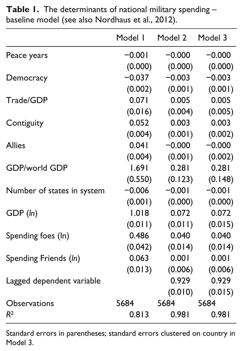
Standard errors in parentheses; standard errors clustered on country in Model 3.

Figure 1.

Coefficient plot of Table 1. Note: horizontal bars pertain to 90% confidence interval; the vertical dashed line signifies a coefficient value of 0.

The results in Table 1 and Figure 1 essentially mirror the findings in Nordhaus et al. (2012) and are in line with the theoretical expectations developed in the literature. Firstly, past military spending is a major determinant of current military investments. Secondly, the log of real GDP, the proxy for the economic size and power of a state, displays the expected positive sign and has a comparatively large coefficient. Thirdly, a country’s investment in defense does not appear to be responsive to the expenditure of friendly nations, but seems to be affected by potential adversaries’ spending. Finally, the higher the GDP/World GDP ratio for a country, the higher its investment in the military. All other variables, while being mostly statistically significant according to conventional levels, display coefficients that are rather small in substance.

Note, however, that Ward et al. (2010) forcefully remind us that empirical results in the form of regression coefficients may not tell us much about the actual influence of specific explanatory variables on military spending: policy prescriptions cannot be based on statistical summaries of probabilistic models. Thus, we now proceed with in-sample predictions, out-of-sample forecasts and Bayesian model averaging. Moving from empirical analyses based on statistical significance to prediction/forecasting serves two purposes. Firstly, it allows us to discriminate among explanatory factors more accurately according to their predictive power. Secondly, it offers a more solid scientific basis for assessing future levels of military spending, which is highly relevant from a policy perspective. In the following, we focus on the third model specification in Table 1 as it appears more conservative than Models 1 and 2.

In-sample prediction

How effective is the model in predicting military spending in-sample? Put differently, how accurate are the “conditional statements about a phenomenon for which the researcher actually has data, i.e., the outcome variable has been observed?” (Bechtel and Leuffen, 2010: 311). To assess this, we compare the predicted yearly median levels of military spending using the estimated parameters from Model 3 with the truly observed levels. The results are depicted in Figure 2: the model fails to predict the military build-up shortly after the Korean War (1954), underpredicts values toward the end of the 1990s, and overpredicts a peak near the end of the Cold War. Still, this figure demonstrates that the predicted values fit the time points of the actually observed data reasonably well.

Figure 2.

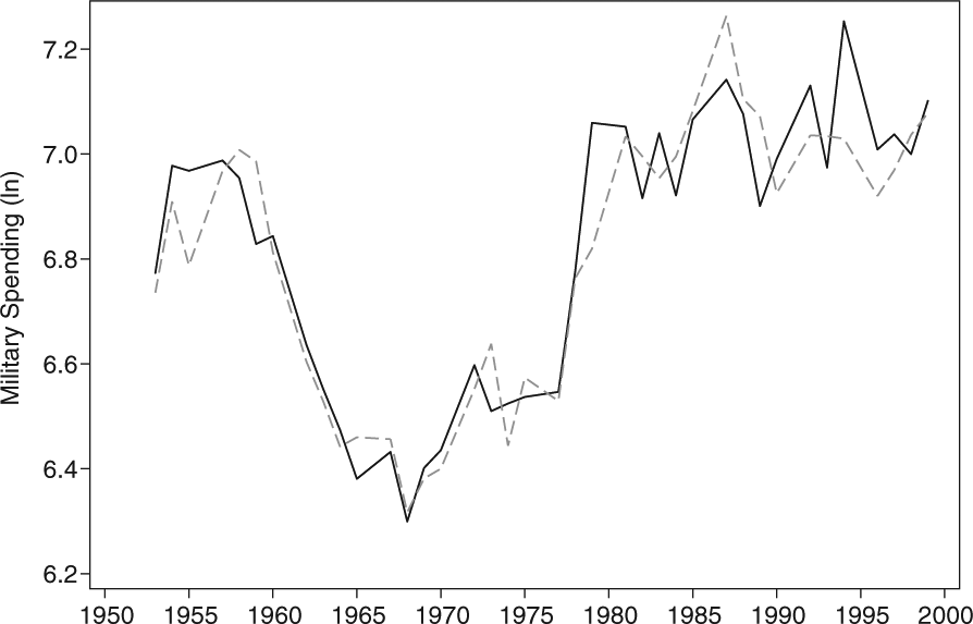
Median levels of military spending: predicted (dashed line) and actual (solid line) values.

To assess the accuracy of this prediction more thoroughly, we use two goodness-of-fit measures: the mean squared prediction error (MSPE) and Theil’s U (Theil et al., 1966), which (unlike the MSPE) does not depend on the scale of the data (see also Bechtel and Leuffen, 2010). Theil’s U is the square root of the ratio between the sum of squared prediction errors of the baseline model (i.e., Model 3) and the sum of squared prediction errors of a naive model, that is, a “no-change prediction” where the level of military spending in t–1 fully corresponds to the level of military spending in t. The closer the MPSE is to 0, the more accurate is the model in making predictions. Moreover, if Theil’s U is larger than 1, the model actually performs worse than the naive model; values for Theil’s U smaller than 1 indicate that the “theoretically informed model” performs better than the naive specification. For our baseline model, the MPSE is 0.0879, while Theil’s U is at 0.9643. Ultimately, therefore, the specifications used in Model 3 perform well in predicting military spending.

Firstly, however, it remains to be seen how accurately this model predicts military spending when moving to the “harder” test of an out-of-sample forecast. Put another way, what is the model’s predictive power when trying to correctly predict military spending that is not “within the very same set of data that was used to generate the models in the first place” (Ward et al., 2010: 8)? Secondly, do some predictors of Model 3 not contribute to the overall predictive power of this model – perhaps despite their statistical significance and the theoretical importance assigned to the sub-indicators of ${\hat{P}}_{i t}^{M I D}$ by Nordhaus et al. (2012) – and may therefore be dropped from the estimation? In order to address both questions, we use out-of-sample forecasting and Bayesian model averaging, the issues considered next.

Out-of-sample forecast

For the out-of-sample forecast, we use a four-fold cross-validation quasi-experimental setup that was repeated 10 times (Ward et al., 2010) – either for the baseline model or a model that omits an explanatory variable from the estimation. Ward et al. (2010: 370) describe this approach in more detail than we can possibly do here due to space limitations. In short, however, this cross-validation randomly divides our 5684 observations we used for Model 3 into four segments. We then use three segments to estimate the parameters, while the fourth segment, also called the “test set” (Ward et al., 2010: 370), is retained for assessing the predictive power of the the baseline model or a model that omits one of the predictors at each time on the pooled subsets. We drop one independent variable from the model at a time in order to estimate the effect that this specific variable has on the model’s ability to make out-of-sample forecasts. Again, we calculated the MPSE and Theil’s U for measuring the predictive power, for which we then present the average values over the 10 repetitions.

Table 2 gives an overview of the baseline model’s out-of-sample forecasting power and the individual contribution each of the variables makes. These contributions are measured in terms of the difference between the average value of the baseline model’s MSPE or Theil’s U values on one hand and, on the other hand, the corresponding average goodness-of-fit measure’s value calculated for a model that discards that particular item. For example, excluding Peace Years from the baseline model leads to an increase in Theil’s U from 0.9675 to 0.9678. Therefore, Peace Years does contribute to the model’s overall prediction and forecasting power by 0.0003 units according to Theil’s U. Similarly, leaving out this variable induces an increase of 0.0001 in terms of the MSPE. The contribution of Peace Years to the model’s forecasting power is therefore given, yet is small in substance, and this mirrors the findings for most other predictors. Five variables constitute an exception to this, though, as these seem to be major contributors to the model’s forecasting power: Democracy, Number of States in System, GDP (ln), Spending Foes (ln) and the lagged dependent variable. Overall, the four-fold cross-validation suggests that these five contribute the most to the overall predictive power of the baseline model taken from Nordhaus et al. (2012).

Table 2.

Out-of-sample forecasting power.

Excluded variable	Mean U	Mean MSPE	ΔU	ΔMSPE
None (baseline model)	0.9675	0.0885	−	−
Peace years	0.9678	0.0886	0.0003	0.0001
Democracy	0.9704	0.0891	0.0029	0.0005
Trade/GDP	0.9675	0.0885	0.0001	0.0000
Contiguity	0.9677	0.0886	0.0003	0.0001
Allies	0.9677	0.0886	0.0002	0.0000
GDP/world GDP	0.9675	0.0885	0.0000	0.0000
Number of states in system	0.9692	0.0888	0.0018	0.0003
GDP (ln)	0.9823	0.0913	0.0149	0.0027
Spending foes (ln)	0.9692	0.0888	0.0018	0.0003
Spending friends (ln)	0.9675	0.0885	0.0001	0.0000
Lagged dependent variable	3.0286	0.8674	2.0611	0.7789

Two additional conclusions can be derived from these findings. Firstly, none of the included predictors in Model 3 actually worsens the forecasting power; that is, neither Theil’s U nor the MSPE decrease when leaving out an item from the model specification and running the four-fold cross-validation. While this may constitute “good news”, note that there are several variables that are unlikely to have any impact on the forecasting power at all. Secondly, those five variables that our out-of-sample analysis highlights as the most important factors for predicting and forecasting future national military expenditure largely pertain to the economic size of a country and its regime type. Most of the proxies for the international security environment, which is treated as one of the core factors in, for example, Nordhaus et al. (2012), are unlikely to matter – the military spending of foes and the total number of states in the international system are the only exceptions. This highlights (again) not only the importance of going beyond statistically significant coefficients, but also that it was crucial to actually disaggregate the MID involvement indicator used by Nordhaus et al. (2012).

Bayesian model averaging

The four-fold cross-validation approach in the previous section does not necessarily suggest that one should drop any variable from our baseline model in order to maximize accuracy in predictions and forecasts; however, some variables hardly make any contribution at all to the forecasting power and may therefore be dropped, even if only for efficiency reasons. To further examine this issue, we implement a final methodological approach that similarly addresses both model and parameter uncertainty: Bayesian model averaging (Amini and Parmeter, 2011; Fernández et al., 2001; Ley and Steel, 2009; Montgomery and Nyhan, 2010; Raftery et al., 1997; Steel, 2014; Zeugner, 2012). A detailed and formal overview of this method is given in the provided references. In brief, however, Bayesian model averaging deals with the uncertainty about one model specification – one specification that may be only one out of many. Inferences based on one model only, however, might be limited and, thus, they should rather reflect the ambiguity about the model. Bayesian model averaging addresses this by considering all possible combinations of variables (in our case, there is a model space of 2048 different models, as we have 11 predictors) in order to increase model fit, that is, “all inference is averaged over models, using the corresponding posterior model probabilities as weights” (Fernández et al., 2001: 564), via goodness-of-fit measures such as the Akaike Information Criterion (AIC) or the Bayesian Information Criterion (BIC), while taking the entire predictive distribution into account (Raftery, 1995; Steel, 2014). To this end, we first assign a prior to the model space, while the data will then lead to a posterior probability, which can be used to identify the “best” model that is usually the one with the highest posterior probability. Bayesian model averaging then uses these posterior model probabilities as weights in order to mix over models (Steel, 2014: 4). Ultimately, we are thus able to calculate posterior inclusion probabilities (PIPs), that is, the sum of posterior model probabilities for all models where a covariate was included (Amini and Parmeter, 2011), for entire models or single predictors in order to determine, in turn, which variables should be incorporated in a model and which ones can safely be ignored.

Figure 3 summarizes the predictors’ PIPs for five different specifications, that is, uniform, Bayesian (or) Risk Inflation Criterion (BRIC), fixed, PIP and random, of the Bayesian model averaging using the BMS package in R (Zeugner, 2012). These five specifications essentially pertain to alternative settings of the (unit information) priors that we assign to the 2048 models or the different predictors ex-ante. This is important, as the use of different prior assumptions can lead to very different results (Steel, 2014: 2). In more detail, apart from the BRIC specification, all setups rely on Zellner’s g-prior as the unit information prior, while uniform has a uniform model prior, fixed has a binomial model prior, PIP assigns a prior inclusion probability of 10% for the lagged dependent variable and 50% for all other covariates⁴ and random assigns a beta-binomial model prior. Finally, BRIC has a uniform model prior, but relies on a Markov Chain Monte Carlo (MCMC) sampling technique, that is, “the birth-death sampler” in our case (Zeugner, 2012: 11), and ensures that the posterior model probabilities asymptotically either behave like the BRIC (Zeugner, 2012: 11).

Figure 3.

Bayesian model averaging – posterior inclusion probabilities.

The results in Figure 3 are highly robust across prior specifications and shed more light on the findings we obtained from the four-fold cross-validation. Specifically, Democracy, Number of States in System, GDP (ln) and the lagged dependent variable are characterized by PIPs that are close to 1.00, meaning that the sum of posterior model probabilities for all models wherein these predictors were included is consistently at or close to 100%. Moreover, Spending Foes (ln) and Peace Years have PIPs that are on average higher than 0.50, that is, the sum of posterior model probabilities for all models wherein these predictors were included is consistently at or close to 50%. All other predictors display PIPs that are, sometimes quite substantially well, below 0.50 and we thus drop these for the final model. Interestingly, apart from Spending Friends (ln), dyadic versions of all variables we drop for the final model are actually included in ${\hat{P}}_{i t}^{M I D}$ , the ex-ante probability of a country being involved in a MID (Nordhaus et al., 2012). This highlights one more time the importance of disaggregating this variable and going beyond Nordhaus et al. (2012)

Discussion and conclusion

In light of the previous sections, we re-estimated the baseline model while leaving out the weakest predictors, that is, Contiguity, GDP/World GDP, Trade/GDP, Spending Friends (ln) and Allies. Afterwards, we performed another round of four-fold cross-validations that we repeated again 10 times (Ward et al., 2010) – either for the original baseline model or the new model that now omits the five weakest predictors. When assessing the predictive power of the latter specification, both the MSPE and Theil’s U should have lower values than the original model if the new, and arguably more parsimonious model, is more powerful in predicting and forecasting future values of military spending. Table 3 summarizes our findings. This table clearly shows that the newly specified, alternative baseline model, which omits five predictors of the original baseline model, is not only more parsimonious, but also slightly more accurate than the model’s original specification: the MSPE is lower by −0.0001, while Theil’s U is −0.0005 units smaller than the original baseline model’s value.

Table 3.

Out-of-sample forecasting power – baseline model versus final model.

Specification	Mean U	Mean MSPE	ΔU	ΔMSPE
Baseline model	0.9675	0.0885	−	−
Final model	0.9670	0.0884	−0.0005	−0.0001

To conclude, we assessed whether important drivers of military expenditure put forward by the existent literature allow us to predict and forecast future levels of national investment in the military. We focused on a recent model by Nordhaus et al. (2012) by using data on 141 countries in 1952–2000. Our results show that most of the explanatory variables perform relatively well in the out-of-sample prediction and the Bayesian model averaging.

Testing the validity of existing theoretical accounts has important implications for theory development and can also offer significant benefits for policymakers in terms of effectively allocating scarce resources to the many areas of government spending. Specifically, our research finds that previous levels of military spending as well as a country’s institutional and economic characteristics particularly improve our ability to predict future levels of investment in the military. Variables pertaining to the international security environment also matter, but seem less important. Given that most, if not all, of the best predictors we identified are either (largely) time-invariant or known ex-ante, we strongly believe that our work helps scholars and policymakers alike to foresee states’ military expenditures more accurately.

In light of this, using the new model, we also assess the prediction and forecasting power for individual countries. This gives us a more accurate idea of where the “good” predictions come from and whether the fairly high levels of prediction/forecasting accuracy are driven by particular states. It is our hope that this also increases the policy relevance of our research. To this end, we use the new model specifications for a sample that comprises one out of all 141 states only, assessed the prediction power via Theil’s U and the MSPE, and repeated this exercise for all countries in our data. Tables 4 and 5 display our findings as we summarize the “top-five” and “worst-five” cases, respectively, in terms of prediction accuracy.

Table 4.

Prediction accuracy by country – top-five states.

Country	Top-5 MSPE	Country	Top-5 U
Iceland	0.0002	Haiti	0.1759
Yemen People’s Rep.	0.0020	Botswana	0.3637
United Kingdom	0.0047	Iceland	0.3796
Italy	0.0050	United Arab Emirates	0.4564
Canada	0.0050	Yemen People’s Rep.	0.4885

Table 5.

Prediction accuracy by country – worst-five states.

Country	Worst-5 MSPE	Country	Worst-5 U
Lesotho	0.8213	Belgium	0.9467
Gambia	0.4001	Denmark	0.9386
Laos	0.3802	Somalia	0.9274
Peru	0.2578	Cameroon	0.9236
Zimbabwe	0.2210	United Kingdom	0.9230

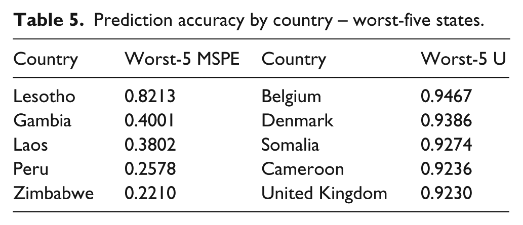
While several conclusions can be derived from these final tables, we would like to highlight two of them. Firstly, despite some exceptions, most of the “top-five” countries are fairly well developed, have a relatively high economic power, and are democracies. Apparently, these characteristics line up well with our strongest predictors identified above and, hence, facilitate accurate forecasts. Similarly, most of the “worst-five” states lack these characteristics, although exceptions do exist here as well. Secondly, somewhat surpirisingly, the United Kingdom is one of the best predictive cases according to the MSPE, but belongs to the worst cases in terms of Theil’s U. While this is arguably driven by some differences for calculating these statistics, also note that Theil’s U for the United Kingdom still is well below 1.00.

Ultimately, we believe that future work should ensure that forecasting becomes a more systematic empirical tool in the current research on countries’ strategic decisions. Similarly, and against this background, next to directly assessing the predictive power of some of the determinants of military spending, our research also sought to further develop the model by Nordhaus et al. (2012). The model that we identified as the new, alternative specification might consequently be used in future research as a baseline model against which to assess new variables of theoretical interest.

Footnotes

Acknowledgements

We would like to thank the anonymous reviewers, Anjali Dayal and the journal’s editor-in-chief, Erik Voeten, for useful comments on an earlier version of this manuscript.

Data and replication information

For this project, we have relied on the data provided by and used the statistical software packages Stata 13 and R for the estimations, figures and tables. All replication material is available in one zip-file from the authors upon publication of this article.

Supplementary Material

The replication file is available at:

Declaration of conflicting interest

The author declares that there is no conflict of interest.

Funding

This research received no specific grant from any funding agency in the public, commercial or not-for-profit sectors.

Notes

References

Aizenman

Glick

(2006) Military expenditure, threats, and growth. Journal of International Trade & Economic Development 15(2): 129–155.

Albalate

Bel

Elias

(2012) Institutional determinants of military spending. Journal of Comparative Economics 40(2): 279–290.

Alptekin

Levine

(2011) Military expenditure and economic growth: A meta-analysis. European Journal of Political Economy 28(4): 636–650.

Amini

Parmeter

(2011) Bayesian model averaging in r. Virginia Polytechnic Institute and University of Miami: Typescript, pp.1–22.

Bechtel

Leuffen

(2010) Forecasting European union politics: Real-time forecasts in political time series analysis. European Union Politics 11(2): 309–327.

Beck

King

Zeng

(2000) Improving quantitative studies of international conflict: A conjecture. American Political Science Review 94(1): 21–35.

Bove

Brauner

(2011) The demand for military expenditure in authoritarian regimes. Birkbeck Working Papers in Economics and Finance (1106).

Bueno de Mesquita

(2011) A new model for predicting policy choices: Preliminary tests. Conflict Management and Peace Science 28(1): 65–87.

Choucri

Robinson

(1978) Forecasting in International Relations: Theory, Methods, Problems, Prospects. San Francisco, CA: W.H. Freeman.

10.

Clayton

Gleditsch

(2013) Will we see helping hands? Predicting the initiation and outcome of civil war mediation. Conflict Management and Peace Science. Available at: http://cmp.sagepub.com/content/early/2013/12/11/0738894213508693.full.pdf.

11.

Collier

Hoeffler

(2006) Military expenditure in post-conflict societies. Economics of Governance 7(1): 89–107.

12.

Dunne

Perlo-Freeman

(2003) The demand for military spending in developing countries: A dynamic panel analysis. Defence and Peace Economics 14(6): 461–474.

13.

Dunne

Perlo-Freeman

Smith

(2008) The demand for military expenditure in developing countries: hostility versus capability. Defence and Peace Economics 19(4): 293–302.

14.

Dunne

Smith

(2010) Military expenditure and granger causality: A critical review. Defence and Peace Economics 21(5–6): 427–441.

15.

Dunne

Smith

Willenbockel

(2005) Models of military expenditure and growth: A critical review. Defence and Peace Economics 16(6): 449–461.

16.

Fernández

Ley

Steel

(2001) Model uncertainty in cross-country growth regressions. Journal of Applied Econometrics 16(5): 563–576.

17.

Gleditsch

Ward

(2013) Forecasting is difficult, especially the future: Using contentious issues to forecast interstate disputes. Journal of Peace Research 50(1): 17–31.

18.

Goldsmith

(2003) Bearing the defense burden, 1886–1989 why spend more? Journal of Conflict Resolution 47(5): 551–573.

19.

Goldstone

Bates

Epstein

. (2010) A global model for forecasting political instability. American Journal of Political Science 54(1): 190–208.

20.

Heo

(2010) The relationship between defense spending and economic growth in the United States. Political Research Quarterly 63(4): 760–770.

21.

Kollias

Paleologou

S-M

(2013) Guns, highways and economic growth in the United States. Economic Modelling 30(3): 449–455.

22.

Ley

Steel

MFJ

(2009) On the effect of prior assumptions in Bayesian model averaging with applications to growth regression. Journal of Applied Econometrics 24(4): 651–674.

23.

Marshall

Jaggers

(2004) POLITY IV Project: Political Regime Characteristics and Transitions. Dataset User’s Manual. College Park, MD: University of Maryland.

24.

Montgomery

Nyhan

(2010) Bayesian model averaging: Theoretical developments and practical applications. Political Analysis 18(2): 245–270.

25.

Nordhaus

Oneal

Russett

(2012) The effects of the international security environment on national military expenditures: A multicountry study. International Organization 66(03): 491–513.

26.

O’Brian

(2010) Crisis early warning and decision support: Contemporary approaches and thoughts on future research. International Studies Review 12(1): 87–104.

27.

Pieroni

(2009) Military expenditure and economic growth. Defence and Peace Economics 20(4): 327–339.

28.

Raftery

(1995) Bayesian model selection in social research. Sociological Methodology 25(2723): 111–164.

29.

Raftery

Madigan

Hoeting

(1997) Bayesian model averaging for linear regression models. Journal of the American Statistical Association 92(437): 179–191.

30.

Schneider

Gleditsch

Carey

(2010) Exploring the past, anticipating the future. International Studies Review 12(1): 1–7.

31.

Schneider

Gleditsch

Carey

(2011) Forecasting in international relations: One quest, three approaches. Conflict Management and Peace Science 28(1): 5–14.

32.

Smith

, (1995) The demand for military expenditure, Handbook of Defense Economics, in: Keith

Hartley

Todd

Sandler

(ed.), Handbook of Defense Economics, edition 1, volume 1, chapter 4: 69–87, Elsevier.

33.

Steel

MFJ

(2014) Bayesian model averaging and forecasting. University of Warwick: Typescript.

34.

Theil

Beerens

Tilanus

. (1966), Applied Economic Forecasting, Vol. 4. Amsterdam: North-Holland Publishing Company.

35.

Ward

Greenhill

Bakke

(2010) The perils of policy by p-value: Predicting civil conflicts. Journal of Peace Research 47(4): 363–375.

36.

Zeugner

(2012) Bayesian model averaging with bms. R Statistical Software Reference Manual, pp.1–35.

Forecasting military expenditure

Abstract

Keywords

Introduction

Data and empirical strategy

In-sample prediction

Out-of-sample forecast

Bayesian model averaging

Discussion and conclusion

Footnotes

Acknowledgements

Data and replication information

Supplementary Material

Declaration of conflicting interest

Funding

Notes

References