
Abstract
This article assesses whether the antimajoritarian outcome in the 2012 US congressional elections was due more to deliberate partisan gerrymandering or asymmetric geographic distribution of partisans. The article first estimates an expected seats–votes slope by fitting past election results to a probit curve, and then measures how well parties performed in 2012 compared to this expectation in each state under various redistricting institutions. I find that while both parties exceeded expectations when controlling the redistricting process, a persistent pro-Republican bias is also present even when maps are drawn by courts or bipartisan agreement. This persistent bias is a greater factor in the nationwide disparity between seats and votes than intentional gerrymandering.
Leading into the 2012 general election in the United States, much of the media’s prognostication focused on the possibility that President Barack Obama might win reelection with a majority of the Electoral College yet a minority of the popular vote. In retrospect, Obama won a comfortable popular vote victory, but the same election saw a parallel “antimajoritarian” outcome in the House Representatives: Republicans won just 49.4% of the aggregated two-party vote and yet won 54% of the seats.
On the surface, Republican partisan gerrymandering appears to explain this disparity. The argument that Democrats underperformed in their seat share due to Republican control of redistricting in many large states is relatively simple. Firstly, it is certainly true that Republicans controlled this process in more states, representing more seats. In addition, in each of these states, Democrats won fewer seats than any reasonable allocation of the popular vote would suggest was “fair.” For example, Republicans won a large majority of the seats in Pennsylvania, North Carolina, and Michigan, despite losing the mean popular vote by district in each state.
However, the problem for Democrats might actually be more fundamental: the current geographic distribution of partisans now leaves Democrats at a disadvantage so long as congressional representation is based on contiguous geographic districts. It is unsurprising that Republicans won more than their fair share of seats in states where they drew the maps. However, Democrats also underperformed under bipartisan maps, and gained only small advantages from their own maps, suggesting their main issue is not gerrymandering, but districting itself.
The observation that Republicans appear to have a natural advantage in the geographic dispersion of their voters is not just a recent one. Erikson studied this phenomenon in northern districts in the 1960s, concluding that “the tendency toward a Republican gerrymander in the distribution of constituency vote” was “the ‘natural’ state of affairs” and “more an accident of geography than the intentional creation of Republican legislatures” (Erikson, 1972: 1241–1243).
In the 1970s, this bias seemed to reverse to the benefit of Democrats, largely due to overwhelming Democratic control of districting in the South (see e.g. Brunell, 1999; McGhee, 2012). In recent years, however, Erikson’s thesis has received renewed attention. Hirsch, for example, examines the 2000 redistricting cycle and asserts that “Democratic concentrations in urban areas make it easier for Republicans to gerrymander successfully…[and] relatively harder for Democrats to gerrymander successfully” (Hirsch, 2003: 196). 1 Chen and Rodden (2013) use random districting simulations of Florida and other states to argue that the Democratic Party is disadvantaged even under neutral districting methods, tracing this bias back to urban population shifts during the industrial revolution. In addition, through a case study of several ideologically neutral proposals to redistrict Virginia, Altman and McDonald conclude “there may be some modest truth to the claim that urban Democrats are inefficiently concentrated within their urban communities from a redistricting standpoint” (Altman and McDonald, 2013: 830).
Several recent trends, however, might cast doubt on the lasting relevance of Erikson’s assertion. These include more sophisticated and varied redistricting institutions and tools and changing demographic patterns, particularly the dramatic rise in Hispanic population. This note takes a first cut at adjudicating this question as applied to the 2012 election results.
Estimating the seats–votes curve
To assess the bias in maps of individual states, we must first establish how a “fair” map might translate the popular vote for individual candidates into seats. It has been almost universally observed that electoral systems employing single-member districts yield seat majorities that exaggerate vote majorities (Lijphart, 1999; McDonald, 2009; Rae, 1967). To the extent that this exaggeration is not biased to favor one party, it is often seen as a feature of such systems rather than a bug, creating governing mandates out of what would otherwise be the confusion of unstable plurality coalitions. The exaggeration tends to take the shape of a probit or logit function, although the slope (i.e. the sensitivity) of the curve has been found to vary widely among electoral systems (e.g. King and Browning, 1987; Taagepera and Shugart, 1989; Tufte, 1973).
Tufte (1973) proposed that a system of districting must pass two tests to be “minimally democratic.” Firstly, it must be responsive such that an increase in votes for one party will translate into an increase in seats, and secondly, it must be unbiased in treating both parties alike. We therefore start from the premise that a fair assignment of seats to parties will be not be biased in favor of one party, but also will not require proportional representation. Rather, we will assume that a party should expect to win a proportion of seats in line with historical patterns found in modern congressional elections.
The “fair expectation” for seats given a vote share is thus estimated by imputing a responsiveness slope that is average for all congressional elections since the nationwide implementation of equal-population districts. Figure 1 shows the relationship between national vote share and seats won in congressional elections since 1972, as well as a fit line using both probit (solid line) and ordinary least squares (OLS; dashed line). Within the observed range, these two methods yield almost identical results, indicating that a 1% increase in vote share will produce about a 2% increase in seat share. Thus, winning 55% of the vote will generally yield about 60% of the seats. 2 The estimated 2012 result (not included in the fit line) falls far below this line, demonstrating the Democrats’ underperformance compared with historical averages.

Seats–votes curve in US congressional elections, 1972–2012.
The probit curve has a slope coefficient of 0.026, representing responsiveness, and a constant of −0.040 (where the independent variable is the Republican percentage point advantage in the aggregated popular vote, and the dependent variable is share of seats won). This coefficient of 0.026 is used throughout the analysis to represent the “expected” responsiveness of the seats–votes curve, equivalent to the ρ term in King and Browning’s (1987) model. 3
In lieu of using national election data to measure the responsiveness of congressional seats to votes, we can alternately estimate this slope using state-by-state election data from the same 1972–2010 period, using mean two-party vote share by district as the independent variable, and statewide seat share as the dependent variable, similar to the 2012 results presented below. This method (detailed in Table A1 of Supplementary Material) yields a slope coefficient of 0.0234. In addition, unopposed races in the South, particularly in the first two decades, distort this result: the coefficient estimate is 0.0271 if the South is excluded. 4 Using this method, we can also include fixed effects for decade, none of which are significant. Although the bias in congressional maps appears to vary over time, there is little variation in responsiveness, either within this period or when comparing the last 40 years to earlier decades in the 20th century. Imputing the lowest slope value under this method (0.0234) still yields substantively very similar results (shown in Table A2 of Supplementary Material).
Methodology for vote share and seat share
Drawing on the 2012 election results, I have calculated each party’s mean vote share across each state’s congressional districts, using mean rather than the aggregate share so that each district is weighted equally regardless of turnout and unopposed races can be included. Where a candidate ran completely unopposed, I have assigned that candidate’s party 100% of the vote; where a candidate ran against only minor parties, I have assigned the opposing party the vote share of the minor candidates. I then compare the mean vote share with the expected seat share under a “fair” map with zero bias and a historically average seats–votes curve. For example, Michigan Democrats won a mean vote share of 53%, which, when we apply the slope estimate above, translates into winning 56% of seats. In actuality, however, Democrats won only 5 of Michigan’s 14 seats (36%), 20% less than the expected number of seats in that state.
Each state is coded for redistricting control by Republicans, Democrats, or some other institution (e.g. commission, court, bipartisan agreement) to assess whether Republicans exceeded their expected seat share more when they controlled the redistricting process. Table 1 shows bias results for five categories of states, with negative numbers in the last column indicating the degree of pro-Republican bias. The first three subheads show states with at least six congressional districts with maps drawn by Republicans, Democrats, and bipartisan agreement/courts, respectively, while the last two subheads show states with the largest Hispanic populations and those in the Deep South, categories that will be analyzed separately.
Seats won versus mean vote share by gerrymandering party: 2012 congressional elections.

Seats won versus seats expected by redistricting control
If the overall pro-Republican bias in the national election outcome was due predominantly to Republicans controlling the districting process in more states, we should expect to observe opposing biases of similar magnitudes in individual states when Republicans and Democrats controlled the process. In addition, we would expect little or no bias in states where maps were drawn by courts or bipartisan agreement. At first glance, neither of these hypotheses seems true.
In every state districted by Republicans, Democrats won fewer seats than their historical expectation, and in six cases they underperformed by 20% or more. It appears as though Republicans gained dramatic benefits across the board from holding the reins of districting.
In contrast, Democrats only slightly exceeded their expected seat share in the three states—Illinois, Massachusetts, and Maryland—where they controlled the process, gaining just a fractional seat above expectation in each. For instance, Illinois Democrats won a smaller majority in their delegation than Republicans won in Pennsylvania or Ohio, despite winning a much larger vote share. Although winning all of Massachusetts’ nine districts may seem a wildly inequitable distribution, by winning 76% of the mean vote Massachusetts Democrats could expect to win 91% of the seats under a “fair” map. If John Tierney had won 1% less in his MA-6 race, Democrats would have slightly underperformed their expected share. 5 While Democrats underperformed by an average of 19% under Republican gerrymanders, they only exceeded expectation by 5% under these Democratic gerrymanders.
In addition, we observe bias even where we should expect none in the redistricting process. Democrats also fell short of expectation in several states with bipartisan or court-drawn maps. For example, despite a constitutional amendment prohibiting Republican legislators from using partisanship to draw maps in Florida, the GOP nevertheless managed to win 17 seats with 51.4% of the vote, surpassing expectation by 2.5 seats. Even under bipartisan gerrymandering in New York, in which Democrats won 21 of 27 seats, their vote share suggested they should have won 22. Across the seven states with bipartisan or court gerrymanders, Republicans exceeded expectation by an average of 7%. 6
So how many seats did this underlying disadvantage cost the Democrats? If we imagine that these bipartisan or court maps were unbiased, and that Democrats and Republicans received equal benefit from their own maps (for example, a 12% advantage as an average), this would have yielded 16 or 17 additional seats, likely getting the Democrats within a couple seats of the majority. By contrast, the disparity between the number of seats gerrymandered by Republicans compared to Democrats likely costs Democrats about nine seats. 7 This initial analysis reveals that geography is a slightly greater factor than intentional gerrymandering in explaining why Democrats won fewer seats than expected from their vote share.
If there is any area of the country where the geographic distribution of partisans has not led to an underrepresentation of Democrats, we might expect to observe it where Democratic voting strength does not hew as closely to the black/white or urban/rural divide. In particular, we find this pattern interrupted in areas with very large Hispanic populations, as Hispanics tend to be both less saturated in their support for Democrats and more geographically dispersed than African-Americans living in large urban areas. In the five states with the highest proportion of Hispanics (Arizona, California, New Mexico, Nevada, and Texas), Democrats won a seat share very close to expectation in each state, despite not controlling the process in any of them. It is possible that non-partisan commissions in California and Arizona may have contributed to greater fairness, but the ease of drawing geographically large, majority Hispanic districts in these states, (e.g. AZ-4, CA-16, CA-51, and TX-23) might have also mitigated the advantage Republicans have in other regions given the distribution of their voters.
The final subhead of Table 1 depicts results from five states in the Deep South. In these states, voting is highly racial polarized and, unlike most of the rest of the nation, much of the African-American population is rural. In addition, amendments to the Voting Rights Act (VRA) have been interpreted to require the drawing of African-American-majority or African-American-influence districts across rural parts of these states, with district maps requiring Department of Justice preclearance under the VRA. Past research has suggested that this may constrain maps to resemble Republican gerrymanders even when drawn by another party (Goedert, 2012; Hill, 1995; Lublin, 1999), and we do see that results in these states are slightly biased against Democrats with one exception. 8 Because we therefore might expect these states to be much differently impacted by both urbanization and the gerrymandering party compared to the rest of the nation, they are excluded from the regression analysis below.
Regression results
To more directly approach Chen and Rodden’s (2013) argument that Democrats are disadvantaged due to their heavy concentration in cities, I analyzed these results using an OLS regression, including 2010 US Census data on race and urbanization. Table 2 depicts regression results with each state weighted by number of districts, excluding five Deep South states and states with only one or two districts. The dependent variable is the difference between Democratic seats won and the number of seats expected given their vote share. A high positive value is a map distorted in favor of Democrats, while a high negative value is a map distorted in favor of Republicans. Dummy variables are assigned for partisan redistricting procedures; the excluded category is bipartisan or court-drawn maps. In addition, controls are included in some models for the percent of the population that lives in urban areas or that is African-American or Hispanic. The “Hispanic Dummy” in Model 1 is a “1” for the five most heavily Hispanic states.
Regression results.
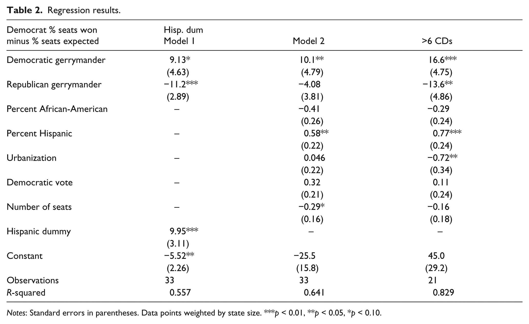
Notes: Standard errors in parentheses. Data points weighted by state size. ***p < 0.01, **p < 0.05, *p < 0.10.
Model 1 reaffirms the three central conclusions from Table 1. Firstly, the effect of partisan control of the districting process is significant and in the expected direction. Secondly, as we can see from the negative and significant constant, which captures the bias in states with a bipartisan or court-drawn map and without a large Hispanic population, maps are distorted in favor of Republicans even when we control for partisan gerrymanders. Finally, this distortion is not present in the case of the most heavily Hispanic states.
Model 2 tests the effect of minority population proportions, includes controls for state size and overall partisanship of the state, and also yields a closer test of the Chen and Rodden (2013) hypothesis by including the urbanization variable. Chen and Rodden hypothesize that the distortion is due to population shifts toward urban areas. If this were true, we would expect more distortion against Democrats in heavily urbanized states. Consistent with Table 1 and Model 1, a larger Hispanic population reduces bias against Democrats, but the size of the African-American population has no significant effect on distortion, and we see no effect for urbanization. 9
Model 3, including only states with more than six districts, paints a different picture, showing a significant negative coefficient for urbanization. Among larger states, which likely include both urban and rural areas, heavily urbanized states (e.g. New Jersey and Pennsylvania) are more often heavily distorted against Democrats than more rural states (e.g. Minnesota and Wisconsin) after controlling for the gerrymandering party. Furthermore, the coefficients for partisan maps increase when we limit the sample to larger states, possibly indicating the greater flexibility parties have in drawing districts in such states. 10
Robustness check: Presidential election results
Although the current congressional map has thus far only seen one cycle of election results, there has been another election held across all 435 of these districts that we can use to test the robustness of this paper’s finding: the 2012 presidential election. Despite winning with 52.0% of the two-party popular vote, Obama won only 209 congressional districts, further suggesting pro-Republican bias. We can substitute Obama’s margin for the congressional election result to measure bias under the various redistricting regimes.
The results of replicating Table 1 using presidential election results are summarized in Table 3 and are detailed in Table A3 of Supplementary Material. In the case of partisan maps and heavily Hispanic states, the average bias is very similar to the bias under the actual congressional election results. Notably, the difference in bias between Republican and Democratic gerrymanders remains the same at 14%. However, the pro-Republican bias under bipartisan and court gerrymanders largely disappears. There are likely two explanations for this difference. Firstly, President Obama won three districts in Minnesota and five districts in New York with 52% or less of the vote, which might be described as luck. However, this result also suggests that the asymmetry in the geographic distribution of partisans is not constant across states and regions. In some “bluish” states, the more conservative areas such as upstate New York and rural Minnesota may be only marginally Republican. These districts may be won by Republicans in a nationally tied electoral environment but captured by Democrats in a climate somewhat more favorable to them, such as Obama’s 4% popular vote victory. In contrast, in the Deep South where the more conservative regions are deeper “red,” probably exaggerated by VRA considerations, the bias against Democrats is actually exacerbated as their vote majority increases.
Seats won versus mean vote share by gerrymandering party: 2012 presidential vote (summary).

Conclusion
Both the state-by-state results and aggregated regression analysis suggest that while deliberate partisan gerrymandering produces additional seats for the districting party, partisan gerrymandering is not a sufficient explanation for the overall antimajoritarian outcome. Instead, pro-Republican bias is observed under all districting regimes. In addition, the regression results offer possible support for the Chen and Rodden (2013) thesis that urbanization has created bias while also forecasting its possible demise if patterns of rapid Hispanic population growth continue.
It is important to note the limits to these conclusions. Firstly, while asymmetric population distributions are a plausible explanation for persistent bias, and one supported by previous research, they are not the only possible cause. For example, one might claim that incumbency could give Republicans advantages in more marginal districts (see McGhee, 2012). This article does not attempt to isolate that cause. 11
This analysis does not imply that Democrats are doomed to the minority even for the next decade. It does indicate they are unlikely to retake the House in an essentially tied national election. Yet national elections are not usually this close: Democrats reversed a Republican gerrymander in Pennsylvania, Virginia, Ohio, and Michigan in 2006 or 2008 (all states with aggressive Republican maps). The 2012 maps leave the Democratic Party several openings; for example, Republicans now sit in five Pennsylvania districts won by Obama in 2008. To win these seats, Democrats will need the electorate to look like 2006 or 2008, but this is far from unprecedented: Democrats won the popular vote by at least 5 points in 12 of the last 20 cycles. But given the unequal concentrations of vote share in most states, not just those with Republican gerrymanders, a Democratic majority will be a bit more difficult than it should be.