
Abstract
This note observes that the pro-Republican bias in the relationship between seats and votes that characterized the 2012 US congressional elections largely disappeared in the 2014 elections, where Republicans won a six-point victory in the national popular vote but only a handful of additional seats. Replicating analysis from an earlier article on the 2012 elections, I find that the source of the decline in bias supports two theories about the effects of gerrymandering and geography on the US Congress. First, bias declined most sharply in states where maps were drawn by Republicans, suggesting that these maps were drawn specifically to maximize seats during a tied national election environment. And second, pro-Republican bias present in bipartisan maps almost entirely disappears, as does the previously observed effect of urbanization on bias, further supporting existing theories about the asymmetric geographic dispersion of partisans.
The 2014 midterm elections were by most measures an unmitigated success for the Republican party. In addition to holding 55 Senate seats and 31 Governorships, Republicans won 247 seats in the House of Representatives – the party’s largest majority since the Great Depression. But these 247 seats represent a surprisingly small gain considering the difference in the national popular vote for Congress between 2012 and 2014. Two years earlier, Republicans won a 33-seat majority despite losing the popular vote by 1%; in 2014, winning the popular vote by almost 6% yielded only an additional 13 seats.
And projections from scholars suggest that the modest Republican House gains may have indeed been surprising too, given the overall size of the Republican wave on other fronts. The October 2014 issue of PS: Political Science and Politics included five short articles predicting the results of the upcoming elections. On the whole, these predictions were quite accurate in estimating a median Republican gain of 14 seats in the House (Campbell, 2014). But while correctly or slightly over-predicting the Republican gains in the House, all three articles addressing Senate races predicted the Republican would pick up fewer than the nine Senate seats that they did (see Abramowitz, 2014; Highton et al., 2014; Lewis-Beck and Tien, 2014). Additionally, Abramowitz estimates that a six-point Republican lead in the Congressional general ballot should result in a 17-seat gain in the House but a seven-seat gain in the Senate.
As discussed in my previous article “Gerrymandering or geography?: How Democrats won the popular vote but lost the Congress in 2012” (Goedert, 2014), the 2012 congressional election result was strongly biased in favor of the Republicans due to a combination of the asymmetric geographic dispersion of partisan and intentional gerrymandering that the Republican party dominated following the 2010 census. But it seems shortsighted to only judge the overall bias of a map with respect to a single, closely contested election. Indeed, recent scholarship such as that of Stephanopoulos and McGhee (2015) has expanded on the notion that bias should be judged with respect to 50/50 election by measuring vote efficiency in maps across a range of election environments (see also McGhee, 2014). This note replicates my 2012 analysis using the recent election data, and finds that these same factors play a much less certain role in inducing bias during the Republican popular vote wave of 2014, despite the same maps being in effect.
We observe declining bias in both Republican and bipartisan gerrymanders. This result highlights two aspects of the debate over districting bias in the current cycle of congressional districting. First, bias is the product of the interaction of districts with the national election environment, and not stable across all elections. Maps that appear biased when the election is close may also appear fair when one party wins by a sizeable margin (and vice-versa). And second, the absence of bias in 2014, just like the presence of bias in 2012, is explainable by a combination of intentional gerrymandering and the asymmetric distribution of partisans.
National seats–votes curve
In previous research (Goedert 2014), I observed that an historically average seat–votes curve over the past 40 years of US congressional elections can be approximated by a line with a slope of about 2, or a probit curve with a slope of 0.026 (where the independent variable is the Republican advantage in the national popular vote, and the dependent variable is Republican share of seats won). This largely matches the findings over the previous century by Tufte (1973). Figure 1 replicates the same table in Goedert (2014), with the addition of a data point for 2014. While 2012 lies far below both the linear (dashed) and probit (solid) expectation lines, indicating strong Republican bias in the result, 2014 falls much closer to expectation, despite the historically strong Republican seats total. Based on the historical average from 1972 to 2010, Republicans won 22 more seats than expected in 2012, but only five more than expected in 2014.
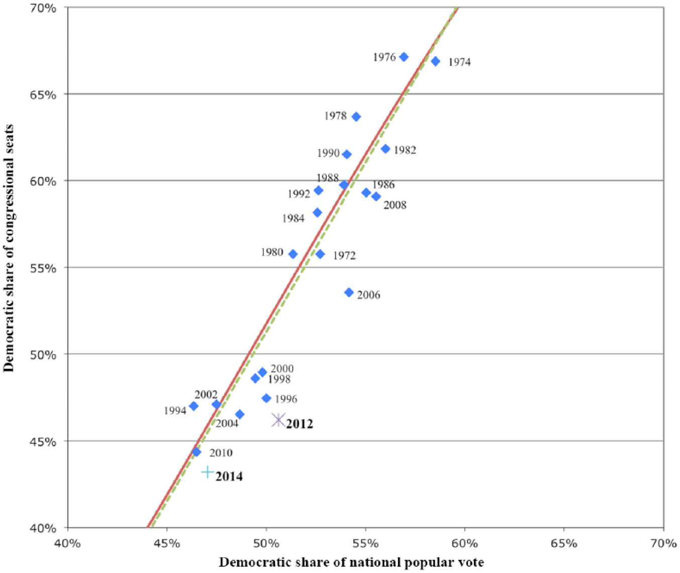
Seats–votes curve in congressional elections 1972–2014.
Given the steep decline in Republican bias on the national level, we should also expect to see this bias disappear in many states whose delegations tilted toward Republicans in 2012. Where should we expect to see bias decline most dramatically? It would be in states where: (1) the partisan allocation of seats was biased toward Republicans in 2012; (2) the vote share for Republicans increased in 2014; and (3) this increase led to few or no additional seats for the GOP in 2014. In moving from an evenly matched election to a moderate Republican wave, we would expect marginally Democratic seats to be most likely to flip to Republicans; states with many such seats would see Republican bias increase in 2014, while states with none of these seats would see bias decrease. In other words, we are most likely looking at states that included very few swing or slightly left-leaning districts. Such a pattern would certainly be predicted in the case of Republican gerrymanders, and thus, we predict that the greatest decline in bias is found in states with Republican maps. However, the “asymmetric dispersion” theory would also predict this pattern of few lean-leaning swing seats in situations where the geographic dispersion of partisans (most states, excepting those with high Hispanic populations) would tend to preclude their creation. So states with bipartisan gerrymanders should also see some decline in the bias generated from asymmetric partisan dispersion, but less than Republican gerrymanders, which deliberately avoid these districts.
In contrast, we would not expect to see bias decline in states containing a lot of slightly Democratic seats that would be vulnerable during a wave like 2014. This would include states with marginally Democratic regions (e.g. rural Hispanics-majority districts) or gerrymanders that would deliberately create them (drawn by Democrats). While Republican bias should not decrease in these states, it is unclear whether it should increase; this would depend on the partisan balance of the state compared to the size of the wave. The reason for this ambiguity is that the few Democratic gerrymanders in the current decade tended to occur in states that already consistently vote heavily Democratic, including Massachusetts and Maryland. It is possible that the Democratic vote is strong enough in these states that even a maximally Democratic gerrymander would not require drawing many marginally Democratic seats, or that the size of even the 2014 wave would not be enough to overcome their existing partisan lean.
Breakdown by gerrymandering regime
Table 1 replicates the same table from Goedert (2014), breaking down individual states by the party responsible for gerrymandering at the start of the decade, with separate categories for states with very high Hispanic populations and Deep South states most affected by the Voting Rights Act constraints (as discussed in Goedert 2014). 1
Seats won vs. mean vote share by gerrymandering party: 2014 congressional elections.

As shown in Table 1, it appears that bias has responded exactly as hypothesized. We immediately see the biggest difference in the Republican gerrymanders, where Democratic vote share fell most steeply (from an average of 48% to 43%), but Republicans collectively gained only one seat. The result is that the pro-GOP bias generated from these maps was reduced by more than half. And the change was quite consistent across states – bias fell by at least 5% in eight of the nine states. In 2012, six of these states saw a Republican bias of at least 20%; in 2014, none of them did. It is still notable that Republican gerrymanders remained biased as a whole, as Republicans of course still win virtually all of the seats except those few deliberately packed with Democrats. The decline in bias is largely due to Republicans winning seats they had already won in 2012, but by larger margins. It may be that bias in swing state Republican gerrymanders could be entirely reversed toward the Democrats under a strong Democratic tide (as was seen in states such as Pennsylvania and Ohio during the 2008 wave election), but this drastic outcome is unlikely during a Republican wave, unless the tide was so strong as to make even the packed Democratic seats competitive.
Bipartisan maps also see bias decline, though to a lesser extent and less predictably than Republican maps. Overall, these maps went from having a 7% Republican bias to less than 2%, now appearing collectively very close to fair. Republicans gained 4% in vote share in these states, and three additional seats, all in New York; overall, both parties won about half the vote and half the seats.
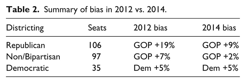
In contrast, we might expect Republicans to gain several seats in Democratic gerrymanders, which generally try to draw slightly pro-Democratic districts to maximize their seat share in close elections. And we see evidence of this in Illinois, the most notable Democratic gerrymander of this decade, where Republicans defeated two incumbents in 2014, destroying the bias that the map generated in 2012. Maryland remains highly biased toward the Democrats, largely because the incumbent in the 6th District survived a shockingly close race by 1%. And the all-Democratic delegation in Massachusetts remained, but their dominant mean vote share predicted that Democrats would win every district in the state anyway. Overall, these states remained slightly biased toward Democrats, as they had in 2014. 2 The summarized results in Table 2 suggest that both the intentional gerrymandering and geographic dispersion sources of bias declined by 5% between 2012 and 2014, from 12% to 7% in the case of gerrymandering, and from 7% to 2% in the case of geography. 3
Summary of bias in 2012 vs. 2014.
The previous article hypothesized that states with the largest Hispanic populations may not have displayed the same Republican bias as other states because Democratic-leaning Hispanics (especially in more rural areas) may have made the drawing of Democratic leaning districts more natural in these states. Conversely, we might expect these same districts to be more vulnerable to a moderate Republican wave. And indeed, Republicans gained a seat in each state of Arizona, Nevada, and Texas in 2014. 4 However, overall bias actually moved slightly in favor of Democrats, largely because Democrats were extremely fortunate to win all seven races decided in California by less than 5%. Bias did not change substantially in the Deep South states because Republican vote share changed very little; we might speculate that vote choice in this region is relatively inelastic.
Regression analysis of urbanization
In the previous article, a regression analysis showed that Republican bias correlated with urbanization among medium and large states in the 2012 elections, as a test of Chen and Rodden’s (2013) theory that urban population patterns generate Republican bias in legislative maps, even under neutral districting procedures. Table 3 replicates that analysis for 2014, with starkly different results. Both the effect of urbanization increasing Republican bias and the effect of Hispanic population decreasing it are reduced to statistically insignificant levels in 2014. The urbanization coefficient declines in 2014 because the forces that created bias in an evenly balanced election (many urban seats won overwhelmingly by Democrats, and less urban seats won narrowly by Republicans) are not as present in an election favoring Republicans. In 2014, those urban seats are still won by Democrats, but less overwhelmingly, while the Republican seats stay Republican by a larger margin. And when urbanization is no longer significantly associated with bias, the lack of bias among heavily Hispanic states is no longer exceptional, as it was in 2012.
Regression results.

Notes: Standard errors in parentheses. Data points weighted by state size.
p<.01; **p<.05; *p<.10.
And the effects of partisan gerrymandering also become less significant. Although the coefficients on Democratic and Republican gerrymanders decrease only slightly, the uncertainty around them increases – partisan gerrymandering was a less consistent predictor of bias during the Republican wave in 2014 compared to the close election in 2012, a result consistent with state-by-state examples in Table 1. Note that the difference in these coefficients is not significant between 2012 and 2014. However, this is consistent with the general sense that while there is strong evidence of Republican bias due to both gerrymandering and geography, the conclusions we can draw in either direction on either count are much murkier in the case of 2014.
Conclusion
After a startling deviation from historical norms in 2012, the relationship of seats to votes in the 2014 congressional elections returned to a state much closer to expectation. While this evidence remains purely anecdotal based on two consecutive elections, the contrast between them provides further insight as to when to expect to find bias in congressional maps. In particular, the steep decline in bias in Republican-drawn maps suggests they were drawn specifically to maximize seat expectation in a nationally tied election. Additionally, the similar decline in bias in bipartisan maps in a pro-Republican wave election supports the theory that districts are sometimes unintentionally drawn resembling Republican gerrymanders, including many slightly right-leaning seats along with several heavily Democratic seats, due to the geographic dispersion of partisans. This is further supported by the contrasting effect (or lack thereof) of urbanization on bias across these elections.
Finally, the stark differences in results across temporally proximate and superficially similar elections highlights the importance of considering the national election environment, and its potential for wide variation, in evaluating gerrymanders and voting systems. When evaluating the respective effects of intentional gerrymandering and geographic dispersion, it is important to consider the range of possible electoral environments. Partisan gerrymanders may be drawn to be most effective (and most biased) when the national electoral environment is close. But this same circumstance of a tied national election may also yield significant Republican bias due to geographic dispersion, making Democratic gerrymanders seem less effective and Republican maps more effective than they would have been under a different overall environment. So simply evaluating the context of a close national election may not tell the full story.
Moreover, many pundits have predicted a sustained and unbreakable lock on the House of Representatives through the remainder of the decade as a result of the bias observed in 2012. But the Republican wave in 2014 demonstrates that observation is not constant across time, and just as they did in 2008, Democrats could potentially eliminate this bias, due to both gerrymandering and geography, through a wave in their favor in 2016 or beyond.
Footnotes
Declaration of conflicting interest
The author(s) declared no potential conflicts of interest with respect to the research, authorship, and/or publication of this article.
Funding
The author(s) received no financial support for the research, authorship, and/or publication of this article.