Sage Journals: Discover world-class research

Abstract

Background:

Chronic kidney disease, or renal failure, is a public health problem with an estimated prevalence of 8%–16% worldwide. This study was conducted to investigate the evolution of hematocrit levels over time in renal patients after transplantation and to determine how the evolution of hematocrit levels depends on the patients’ age, sex, and other factors.

Objective:

The main objective of this study was to employ a mixed-effects model to examine the unbalanced longitudinal evolution of hematocrit levels in chronic kidney failure patients.

Methodology:

This longitudinal study included 1160 patients who received a renal transplant. These patients were followed for at most 10 years. The hematocrit level was considered the response, while the covariates were time in years, sex, and age of the patients. Different statistical methods, such as explanatory analysis, multivariate regression, two-stage analysis, and linear mixed-effects models, were employed to explore the evolution of hematocrit over time.

Results:

The results revealed that hematocrit levels in kidney transplant patients evolve. The sex and age of the patient significantly affect the evolution of hematocrit levels. Males tend to have a greater increase in hematocrit levels over time than females do. Hematocrit levels tend to increase with increasing age. Furthermore, cardiovascular problems before transplant and rejection symptoms did not significantly affect the evolution of hematocrit levels.

Conclusions:

Hematocrit levels evolve, and this evolution follows a quartic time effect. The change in hematocrit levels varies according to the sex and age of the patient after a kidney transplant. Patients with low hematocrit levels tend to have a greater increase over time.

Keywords

Kidney transplant longitudinal data multivariate model two-stage analysis linear mixed-effects model

Introduction

Chronic kidney disease (CKD) is indeed a noteworthy global health concern, being the 16th leading cause of years of life lost worldwide. It affects approximately 8%–16% of the population, with less than 5% of patients in the early stages aware of their condition. As underlined in earlier systematic reviews, proper screening, diagnosis, and management by primary care clinicians are vital to alleviate confrontational outcomes associated with CKD, such as cardiovascular disease and end-stage kidney disease.¹

CKD is a global public health concern, with an estimated incidence of 8%–16% worldwide, posing considerable challenges to healthcare systems because of its progressive nature and related.^2–4 Kidney failure (stage G5) is the most severe stage of CKD, necessitating renal replacement therapy, such as dialysis or transplantation.⁵ Anemia is a common CKD consequence that is significantly connected to poor clinical outcomes, such as faster disease progression, cardiovascular problems, and decreased quality of life.⁶

The occurrence of chronic renal insufficiency has increased noticeably, with estimates signifying that from 1978 to 1991, the number of adults aged 20–74 years with chronic renal insufficiency rose from 2.6 to 3.9 million, corresponding to a rise in prevalence from 1970 to 2460 per 100,000 persons. This rise in chronic renal insufficiency is paralleled by an alarming increase in end-stage renal disease (ESRD) incidence, where for every 1000 adults with chronic renal insufficiency in 1978, there were 9 new cases of ESRD by 1983, compared to 16 new cases per 1000 adults by 1996.⁷

Hematocrit levels, which characterize the percentage of blood volume occupied by red blood cells, are vital pointers of anemia in CKD patients. Among patients with chronic renal insufficiency, hematocrit levels can decline from approximately 39% to 30% as estimated glomerular filtration rate drops from 60 to 30 mL/min/1.73 m². In patients with ESRD, hematocrit levels may collapse to as low as 25%–30%, underlining the significance of monitoring and managing these levels to avoid adverse consequences such as cardiovascular disease and increased mortality.⁸ Hematocrit levels, which measure the fraction of red blood cells in the blood, are important indicators for monitoring anemia in CKD patients. However, the longitudinal evolution of hematocrit levels in CKD patients, particularly those approaching kidney failure or receiving renal transplantation, is poorly understood. Hematocrit levels are defined as the proportion, by volume, of the blood that consists of red blood cells. According to Vlahakos et al.,⁹ the normal range for hematocrit differs by sex; it is approximately 45%–52% for males and 37%–48% for females. This knowledge gap impairs the ability to predict and manage complications such as posttransplant erythrocytosis (PTE), a condition characterized by persistently elevated hematocrit levels above 51%, which is more common in males and usually occurs within 2 years of transplantation.⁹

The evolution of hematocrit levels in CKD patients is regulated by a complex interaction of factors, including renal function, inflammation, concomitant diseases, such as diabetes and hypertension, and treatment modalities. Traditional statistical methods, such as linear regression, are sometimes insufficient for assessing longitudinal data in clinical settings because they fail to account for imbalanced follow-up schedules, missing data, and individual variability.¹⁰

These constraints are more obvious in CKD studies, as patients may have irregular follow-up visits and different disease progression trajectories. Mixed-effects models, which include both fixed and random effects, provide a strong foundation for assessing such unbalanced longitudinal data by accounting for within- and between-subject variability and clustering.¹¹ Unlike classic regression models, which presume observation independence and fail to handle correlated data, mixed-effects models are explicitly built to overcome these issues, making them excellent for assessing longitudinal data in clinical research.¹²

The primary goal of this study was to use a mixed-effects model to look at the imbalanced longitudinal evolution of hematocrit levels in chronic kidney failure patients. The project specifically intends to answer the following research questions: (1) How do hematocrit levels evolve in chronic renal failure patients over time? (2) How much individual variability exists in hematocrit level progression, especially when irregular follow-up periods are considered? (3) What factors influence the evolution of hematocrit levels in chronic renal failure patients? The goal of this study is to provide a thorough understanding of hematocrit trajectories and their drivers, resulting in insights that can inform tailored treatment options and enhance patient outcomes.

In this study, the dependent variable was the hematocrit level of chronic renal failure patients, an important predictor of anemia and overall blood health. The predictors include log-transformed time (log(year + 1)), which accounts for the nonlinear evolution of hematocrit levels over time; age, which reflects the potential impact of aging on renal function and hematocrit levels; and sex (male = 1, female = 0), given the recognized differences in hematocrit levels between males and females¹³. The experience of cardiovascular problems during the year preceding transplantation (cardio: yes = 1, no = 0), as cardiovascular complications, is a major cause of morbidity and mortality in CKD patients¹⁴; and the presence of rejection symptoms during the first 3 months posttransplantation (Reject: yes = 1, no = 0) may influence hematocrit levels due to immune-mediated responses and treatment adjustments.⁹ These factors were chosen for their clinical importance and potential to influence hematocrit evolution in individuals with CKD.

Given the clinical relevance of these results, our study aims to model the longitudinal changes in hematocrit levels in patients with chronic kidney failure using a linear mixed-effects model (LMM). By examining the effects of age, sex, and other factors on hematocrit evolution over time, we seek to address critical gaps in the literature and provide understandings that can enlighten healthier management strategies for CKD patients.

Mixed-effects models are particularly useful in this scenario for various reasons. First, these models can incorporate both fixed effects, which represent predictors with constant values such as age, sex, and baseline renal function, and random effects, which account for variability within clusters such as repeated measurements from the same patient or data collected from multiple centers.¹¹ This dual structure allows the model to capture both overall trends in hematocrit evolution and individual heterogeneity across patients.

Second, mixed-effects models can address imbalanced and missing data, which are common in longitudinal research due to unpredictable follow-up schedules and patient dropout. This flexibility guarantees that the study is not skewed by excluding patients with incomplete data, resulting in a more accurate portrayal of the hematocrit trajectory. Third, mixed-effects models can account for heteroscedasticity or unequal variances in data that are common in clinical settings.¹²

According to Vonesh et al.,¹² the mixed-effects models are preferable to classic regression methods in this study because they solve these methodological problems and provide a more robust and comprehensive examination of longitudinal data.

The study’s relevance stems from its ability to fill important gaps in CKD research and therapeutic practice. First, using a mixed-effects modeling approach to evaluate unbalanced longitudinal data results in a more rigorous and comprehensive examination of hematocrit progression, overcoming the limits of traditional statistical methods, including classical regression, logistic regression, and Poisson regression. This methodological breakthrough allows researchers and clinicians to better understand the patterns and determinants of hematocrit changes in CKD patients, particularly those with irregular follow-up schedules.

Second, the findings of this study are predicted to have important therapeutic implications by identifying factors related to aberrant hematocrit levels, such as PTE, and directing targeted anemia treatment interventions. This will eventually lead to better patient care and quality of life for CKD patients.⁶ Third, this study will be useful for policymakers and healthcare planners by identifying risk factors for hematocrit-related problems and driving the establishment of appropriate CKD treatment plans and monitoring systems. Finally, the project will provide a methodological direction to academic researchers, particularly those studying continuous longitudinal outcomes in CKD and other chronic diseases, by demonstrating the use of mixed-effects models in complex clinical settings.¹⁵

The expected outcomes include identifying risk factors for hematocrit-related complications, developing personalized treatment strategies, and establishing a robust statistical framework for analyzing unbalanced longitudinal data in CKD research.^{2,3,6,9,11,12,15–18} These contributions will not only improve CKD patient care but also serve as a platform for future research into the complicated dynamics of chronic disease progression and biomarker development.

By addressing essential research questions and overcoming methodological hurdles, this project will provide practical insights to clinicians, researchers, and policymakers, ultimately leading to better patient outcomes and the global fight against CKD.

Methodology

Introduction

The analysis consisted of exploratory analysis and the fitting of three different models, namely, the multiple linear regression model, the two-stage model, and a LMM, and the results were compared. All the analyses were conducted at the 5% significance level via the R statistical software package.

Research design

The study was structured as a prospective cohort study with a longitudinal process research design. It is an experimental research design with a quantitative research approach for repeatedly measuring continuous response variables, namely, the hematocrit level of chronic kidney failure patients. This study was designed to examine the evolution of hematocrit levels associated with age and sex in chronic kidney failure patients over time.

Different statistical analyses, including both descriptive and inferential statistics, such as summary statistics, data exploration, and model comparison, were used in this study. Data exploration is a very helpful tool in the selection of appropriate models. Thus, the individual profiles plot, the mean profile plot exploring the random effects, and other data exploratory analyses for the datasets have been considered. Overall, based on the data structure with continuous longitudinal outcome, a mixed-effects model was proposed to examine the evolution of hematocrit levels in chronic kidney failure patients. The data analysis tools used in this study were Excel, SPSS, and R, and all analyses were conducted at the 5% level of significance. Model comparison techniques were applied to obtain the best and fittest model for a given dataset.

Finally, in this study, we consider both mixed-effects models under maximum likelihood (ML) and restricted ML estimation, and the models were compared to choose the fittest model. Furthermore, we used Akakie’s information criterion (AIC),¹⁹ the Bayesian information criterion (BIC),²⁰ and log-likelihood to select the fittest model for the given data. In addition, the individual profile plots and the variance structure were used to gain insight into the variability in the data and to determine whether random effects (random intercepts and slopes) were considered in the analysis. The mean structure was used to gain insight into the time function that can be used to model the data. Furthermore, the correlation and/or covariance structure was obtained to determine the type of correlation structure to be considered when modeling the random effects.

Study population and data description

This longitudinal study included 1160 (666 males and 494 females) patients who received a renal transplant and were followed up for 10 years at most. The hematocrit level of the patients at each time point of measurement was considered the response. The measurements were taken at fixed time points every year, except for the first two measurements, which were taken after 6 months in between after the transplant. Patient age, sex (male = 1 and female = 0), experience of cardiovascular problems during the years preceding transplantation (cardio: yes = 1 and no = 0), and rejection symptoms during the first 3 months after transplantation (reject: yes = 1 and no = 0) were considered predictors. In addition, the variable time was considered on a log scale (log (years + 1)) in the analysis to improve linearity.⁸

Inclusion-exclusion criteria

Inclusion: This study considered data from a secondary source, and it consists of 1160 (666 males and 494 females) patients who received a renal Transplant and were followed up for a period of 10 years at most.

Exclusion: This study did not conduct any exclusion from the previously collected secondary data; however, previously, the data were collected exclusively from the patients who received a renal transplant and who followed up for a period of at most 10 years.

Study variables

Dependent variable: Hematocrit level of chronic kidney failure patients.

Independent variables: Log (year + 1), age, sex (male = 1, female = 0), experience with cardiovascular problems during the year preceding the transplantation (Cardio: yes = 1, no = 0), and rejection symptoms during the first 3 months after the transplantation took place (Reject: yes = 1, no = 0). The logarithm of the follow-up time in years was considered a random effect, and 1 was added to the years to avoid the undefined or infinity results of the logarithmic function at the baseline follow-up times. The remaining predictors were considered as fixed effects. The age of the patients was measured only at baseline and considered a fixed effect.

Linear mixed-effect model

The use of LMMs in our study is particularly advantageous for several reasons, especially in the context of analyzing longitudinal data in patients with chronic kidney failure. Unlike conventional methods such as logistic regression, which are typically used for binary outcomes, LMMs are designed to handle continuous outcomes and can effectively account for the correlation of repeated measures taken from the same subjects over time.²¹

In our study, hematocrit levels are measured at multiple time points for each patient, creating a hierarchical structure in the data. LMMs allow us to model both fixed effects (e.g. age, sex) and random effects (e.g., individual patient variability), providing a more nuanced understanding of how these factors influence hematocrit levels over time. This flexibility is crucial in clinical settings where individual patient trajectories can vary significantly.

In addition, LMMs can accommodate missing data more effectively than traditional methods, which often require complete cases for analysis. This is particularly relevant in clinical research, where patient drop-out or missed visits can lead to incomplete datasets. By using LMMs, we can include all available data points, thereby maximizing the information extracted from our study population.

In summary, the preference for LMM over logistic regression in our analysis stems from its ability to handle continuous outcomes, account for repeated measures, and manage missing data, making it a robust choice for modeling the longitudinal changes in hematocrit levels in patients with chronic kidney failure.

The linear mixed-effects model for the hematocrit level in chronic kidney failure

Mixed-effect models were developed to handle clustered data and repeated measurements that have been a topic of increasing interest in statistics for the past 40 years.²¹

The mixed-effects models include both fixed and random effects.

Fixed effects: Factors for which the only levels under consideration are contained in the coding of those effects, for instance, sex, where both male and female genders are included in the factor, it is a fixed effect.²¹

Random effects: Factors for which the levels contained in the coding of those factors are a random sample of the total number of levels in the population for that factor. A subject (in this case, ID), which is a random sample of the target population, can be considered random. Through random effects models, the researcher can make inferences over a wider population in the LMM than possible with the Generalized Linear Model (GLM).²¹

The first step in the model-building process for a LMM, after the functional form of the model has been decided, is choosing which parameters in the model, if any, should have a random-effect component included to account for between-group variation.²¹

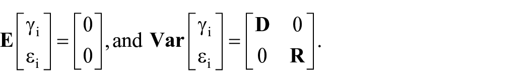
A mixed linear model (LM) is a generalization of the standard LM used in the GLM procedure, the generalization being that the data are permitted to exhibit correlation and non-constant variability. The mixed LM, therefore, provides you with the flexibility of modeling not only the means of your data (as in the standard LM) but also their variances and covariance. The LMM is also a generalization (extension) of the LM that allows for the incorporation of random effects and is represented in its most general fashion²¹:

Y_{i} (t) = X_{i} {(t)}^{T} β + Z_{i} {(t)}^{T} γ_{i} + ε_{i} (t),

where,

$Y_{i} (t)$ : measurement of the univariate response in patient $i^{th}$ at time t.

$X_{i} (t)$ : vector of fixed covariates for the $i^{th}$ subject at time t (of dimension k).

$Z_{i} (t)$ : vector of random covariates for the $i^{th}$ subject at time t (of dimension q).

$β$ : vector of unknown parameters associated with a fixed covariate (of dimension k).

$γ_{i}$ : vector of unknown parameters associated with random covariates for $i^{th}$ subject (of dimension q), $γ_{i} ~ MVN (0, D)$ .

$ε_{i}$ : Random error component.

Furthermore, $Z_{i} (t)$ is a subset of $X_{i} (t)$ and $ε_{i} = {[ε_{i} (t_{1}), ε_{i} (t_{2}), \dots, ε_{i} (t_{n i})]}^{T} ~ MVN (0, R)$ .

$ε_{i}$ is independent of $γ_{i} .$

where $X_{i}$ and $Z_{i}$ are the fixed and random designs of the covariates, respectively; $β$ is a vector of unknown fixed effects; $γ_{i}$ is a vector of unknown random effects; and $ε_{i}$ is the unknown random error. $β$ represents parameters that are the same for all subjects; $γ_{i}$ represents parameters that can vary across subjects.

Terminology:

Fixed effects: $β_{i}$ .

Random effects: $γ_{i} .$

Variance components: elements in D and $R .$

Assumptions:

E [\begin{matrix} γ_{i} \\ ε_{i} \end{matrix}] = [\begin{matrix} 0 \\ 0 \end{matrix}], and V a r [\begin{matrix} γ_{i} \\ ε_{i} \end{matrix}] = [\begin{matrix} D & 0 \\ 0 & R \end{matrix}] .

Assumptions: $Y ~ N (X β, V),$ where $V = Z_{i} D Z_{i}^{'} + R .$

Model-building strategies

A primary goal of model selection is to choose the simplest model that provides the best fit to the observed data. There may be several choices concerning which fixed and random effects should be included in an LMM. There are also many possible choices of covariance structures for the D and $R_{i}$ matrices. All these considerations have an impact on both the estimated marginal mean ( $X_{i}$ ) and the estimated marginal variance‒covariance matrix $V_{i} (= Z_{i} D {Z^{'}}_{i} + R)$ for the observed responses in $Y_{i},$ based on the specified model. The process of building an LMM for a given set of longitudinal or clustered data is an iterative process that requires a series of model-fitting steps and investigations, and the selection of appropriate mean and covariance structures for the observed data. Model building typically involves a balance of statistical and subject matter considerations; there is no single strategy that applies to every application.²¹

Variable selection for fixed and random effects

The top-down strategy: The following broadly defined steps are suggested by Verbeke and Mohlenbergs²¹ for building an LMM for a given dataset. A top-down strategy for model building is used because it involves starting with a model that includes the maximum number of fixed effects that we wish to consider in a model.

Starting with a well-specified mean structure for the model: The modeling process typically begins with specifying an appropriate mean structure, which involves including the fixed effects of as many relevant covariates and their interactions as possible. This ensures that the systematic variation in the response is well accounted for before examining various covariance structures to model the random variation in the data.²¹

Select a structure for the random effects in the model: This step involves the selection of a set of random effects to include in the model. The need to include the selected random effects can be tested by performing restricted maximum likelihood (REML)/ML-based likelihood ratio tests for the associated covariance parameters.²¹

Select a covariance structure for the residuals in the model: Once fixed effects and random effects have been added to the model, the remaining variation in the observed responses is due to residual error, and an appropriate covariance structure for the residuals should be investigated.²¹

Reduce the model: This step involves the use of appropriate statistical tests to determine whether certain fixed-effect parameters are needed in the model.²¹

Estimation methods

Estimation for the mixed-effect model: According to Verbeke and Mohlenbergs,²¹ estimation of the parameters in the LMM is usually based on ML or REML estimation for the marginal distribution of $Y_{i}$ , which can easily be seen as $Y_{i} \sim N (X_{i} β, Z_{i} D Z_{i}^{T} + Σ_{i}) .$ . Note that the LMM implies a model with very specific mean and covariance structures, which may or may not be valid, and hence needs to be checked for every specific dataset at hand. In addition, when $Σ_{i}$ = $σ^{2} I_{n i}$ , with $I_{n i}$ equal to the identity matrix of dimension $n_{i}$ , the observations of subject i are independent of the random effect bi. The model is therefore called the conditional independence model. Even in this simple case, the assumed random-effects structure still imposes a marginal correlation structure for the outcomes $Y_{i j}$ . Indeed, even if all $Σ_{i}$ equal $σ^{2} I_{n i}$ , the covariance matrix in $Y_{i} \sim N (X_{i} β, Z_{i} D Z_{i}^{T} + R$ is not a diagonal matrix, illustrating that, marginally, the repeated measurements $Y_{i j}$ of subject i are not assumed to be uncorrelated. The marginal mean (expected value) and marginal variance‒covariance matrix of the vector $Y_{i}$ are equal to $E (Y_{i}) = X β$ and $V a r (Y_{i}) = V_{i} = Z_{i} D Z_{i}^{T} + R$ .

ML estimation: Suppose that a random sample of N observations is obtained from a linear mixed-effect model as defined above; then, the likelihood of the model parameters, given the vector of N observations, is defined as²¹

\begin{matrix} L = l (β, θ, Y_{i}) = \\ \prod ​ {2 π^{\frac{- n_{i}}{2}} \det {(V_{i})}^{\frac{- 1}{2}} \exp (\frac{- 1}{2} {(Y_{i} - X_{i} β)}^{T} V_{i}^{- 1} (Y_{i} - X_{i} β))} . \end{matrix}

The MLE of $\hat{β}$ is then used to combine all the information from all the N subjects’ equals.

\hat{β} = {(\sum X_{i} V_{i}^{- 1} X_{i})}^{- 1} (\sum X_{i} V_{i}^{- 1} Y_{i}) .

where det refers to the determinant and the elements of the $V_{i}$ matrix are functions of the covariance parameters in Ө.²²

Model comparison technique

To select the best and final model that appropriately fits the given longitudinal data, it is necessary to compare the different models using different techniques and methods. Hence, the models were compared with the AIC, the BIC, and the likelihood ratio test methods for nesting, which were used at a 5% level of significance.²¹

AIC = - 2 \log L + 2 p BIC = - 2 \log Likelihood + n Par \log (N),

where −2 logL is twice the negative log-likelihood value for the model.

P: is the number of estimated parameters.

npar: denotes the total number of parameters in the model

N is the total number of observations used to fit the model. Smaller values of AIC and BIC reflect an overall better fit.

Checking model assumptions for independent mixed models

After fitting an LMM, it is important to carry out model diagnostics to check whether distributional assumptions for the residuals are satisfied, and whether the fit of the model is sensitive to unusual observations. The process of carrying out model diagnostics involves several informal and formal techniques. Diagnostic methods for standard LMs are well established in the statistical literature. By contrast, diagnostics for LMMs are more difficult to perform and interpret because the model itself is more complex due to the presence of random effects and different covariance structures. In this section, we focus on the definitions of a selected set of terms related to residual and influence diagnostics in LMMs.²³ In general, model diagnostics should be part of the model-building process throughout the analysis of a clustered or longitudinal dataset. In this case, only diagnostics for the final fitted model are considered.²¹

Residual diagnostics: Informal techniques are commonly used to check residual diagnostics; these techniques rely on the human mind and eye and are used to decide whether a specific pattern exists in the residuals. In the context of the standard LM, the simplest example is to decide whether a given set of residuals plotted against predicted values represents a random pattern or not. These residual versus fitted plots are used to verify the model assumptions and to detect outliers and potentially influential observations. In general, residuals should be assessed for normality, constant variance, and outliers. In the context of LMMs, we consider conditional residuals and their “studentized” versions.²²

Diagnostics for random effects: The natural choice to diagnose random effects is to consider the empirical Bayes (EB) predictors. EB predictors are also referred to as random-effects predictors or, owing to their properties, empirical best linear unbiased predictors (EBLUPs).²² It is recommended to use standard diagnostic plots (e.g., histograms, Q–Q plots, and scatter plots) to investigate EBLUPs for potential outliers that may warrant further investigation. In general, checking EBLUPs for normality is of limited value because their distribution does not necessarily reflect the true distribution of random effects.

Results and discussion

Results

General data description and summary statistics

To begin with, a general description of the entire dataset, the longitudinal study consisted of 1160 (666 males and 494 females) patients who received a renal transplant and were followed up for 10 years at most. The hematocrit level of the patients at each time point of measurement was considered the response. The measurements were taken at fixed time points every year except for the first two measurements, which were taken after 6 months in between after the transplant. Patient age, sex (male = 1 and female = 0), experience of cardiovascular problems during the years preceding transplantation (cardio: yes = 1 and no = 0), and rejection symptoms during the first 3 months after transplantation (reject: yes = 1 and no = 0) were considered predictors. In addition, the variable time was considered on a log scale (log (years + 1)) in the analysis to improve linearity.

Exploratory data analysis was conducted to investigate various associations, structures, and patterns exhibited in the dataset. This consisted of obtaining summary statistics, such as frequencies and percentages. In addition, individual profile plots, mean structures, correlation structures, and variance structure plots were obtained to gain some insights into the data. The individual profile plots and the variance structure were used to gain insight into the variability in the data and to determine whether random effects (random intercepts and slopes) were considered in the analysis. The mean structure was used to gain insight into the time function that can be used to model the data. Furthermore, the correlation and/or covariance structure was obtained to determine the type of correlation structure to be considered when modeling the random effects.

In addition, the coefficient of multiple determination, the R² meta, and the Fmeta test statistic were applied to explore subject-specific regression models. This was conducted to determine the adequacy of the linear regression model to describe the observed individual proﬁles and the total within-subject variability.

Table 1 illustrates the summary statistics for hematocrit (HCT) levels at each follow-up time point. As a result, the mean HCT levels of chronic kidney failure patients show a notable increase from 31.9% at baseline to approximately 39.7% within the first year, suggesting an early response to treatment. This rise is upheld relatively steadily through year 6, with average evolution values ranging between 38.1% and 40.7%. However, a continuing decline is detected from year 7 onward, with the average HCT declining to 37.1% by year 10. The standard errors decrease over time, showing improved precision of estimates in later follow-ups. These longitudinal trends, characterized by initial improvement followed by a modest decline, underline the need for continued therapeutic intervention and justify the application of a mixed-effects model to account for inter-patient variability and unbalanced measurements over time.

Table 1.

Summary statistics for hematocrit (HCT) levels of chronic kidney failure patients at each follow-up time in year.

Year	Mean_HCT	SE_HCT
0	31.9	0.178
0.5	38.8	0.164
1	39.7	0.173
2	39.7	0.158
3	38.8	0.150
4	38.1	0.156
5	40.7	0.160
6	40.7	0.144
7	37.3	0.141
8	36.4	0.134
9	37.3	0.116
10	37.1	0.100

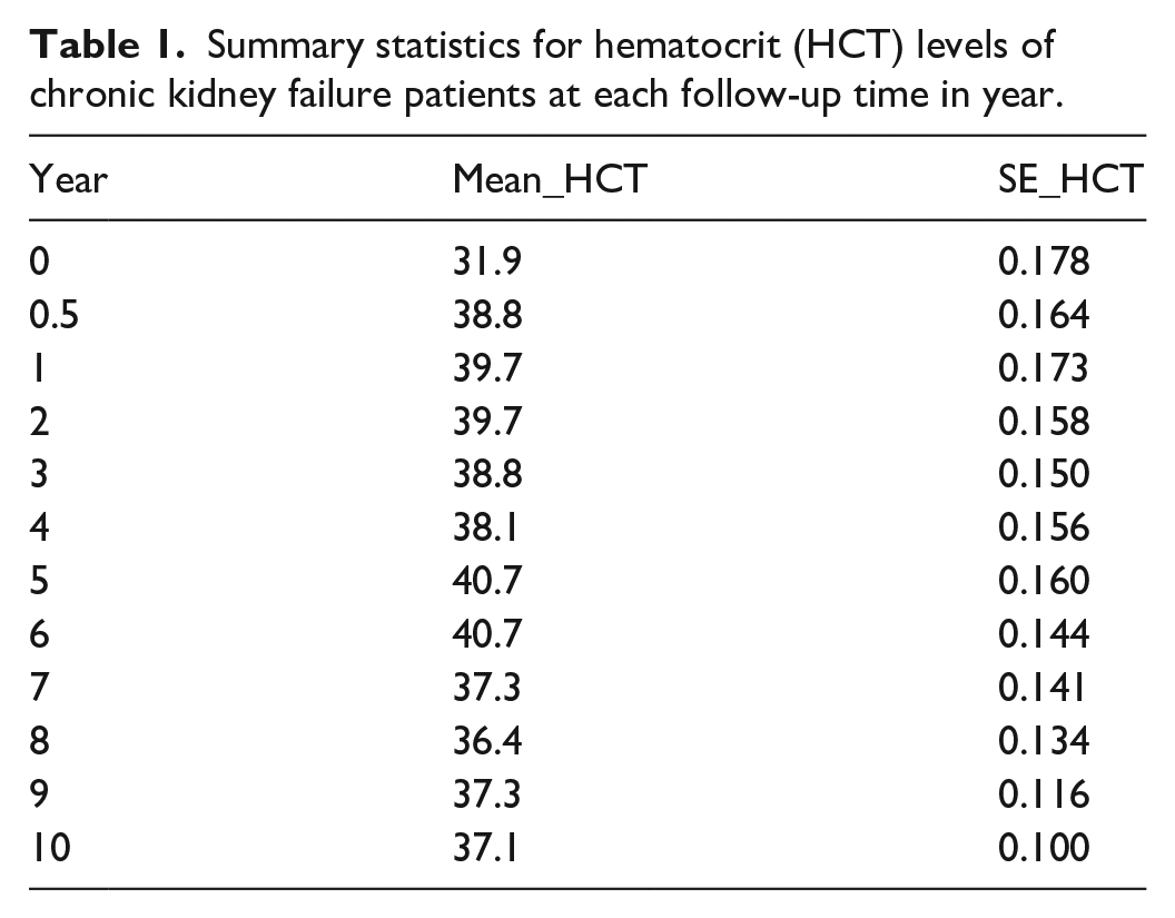
Table 2 illustrates the overall summary of the continuous variables, baseline age, and HCT. The average baseline age of the chronic kidney failure patients is 46.43 years, with a median of 48 and a mode of 54, representing a somewhat left-skewed age distribution intensified in middle to older adulthood. The age interval spans from 15 to 85, with a range age of 70 years, and a standard deviation of 13.30 years, signifying moderate variability. The average evolution of HCT level is 38.04%, close to the median value of 37% and mode of 36%, suggesting a relatively normal or symmetric distribution. The standard deviation of 5.59% imitates moderate dispersion in HCT levels among patients. The small standard errors (0.113 for age and 0.047 for HCT) point out precise estimates of the population means, supporting the reliability of the summary statistics derived from a large sample. These results offer an initial understanding of patient demographic characteristics and hematological status before applying mixed-effects modeling.

Table 2.

Summary statistics for age and hematocrit (HCT).

Variable	Min	Median	Mode	Mean	SD	SE
Age	15	48	54	46.43	13.30	0.113
HCT	14	37	36	38.04	5.59	0.047

Table 3 summarizes the characteristics of summary statistics for continuous variables, age and HCT levels of chronic kidney failure patients. The summary statistics show that both female and male patients show similar age summaries, with identical median ages (48 years) and comparable means (46.2 years for females and 46.6 years for males), proposing a balanced distribution crosswise sexes. The minor dissimilarities in standard deviation and standard error show slightly more variability in male patients’ age but relatively consistent precision in both groups. Regarding HCT levels, males have greater mean (38.7%) and median (38%) values compared to females (mean: 37.1%, median: 36%), proposing probable sex-related physiological or biological differences or responses to treatment. Both groups share the same mode of 36%. The standard errors are comparatively small for both sexes, showing precise estimates. These differences underscore the significance of including sex as a factor in modeling the longitudinal evolution of HCT levels in chronic kidney failure patients.

Table 3.

Summary statistics of age and hematocrit (HCT) by sex.

Sex	Variable	Min	Median	Mode	Mean	SD	SE
Female	Age	17	48	50	46.2	13.2	0.171
Male	Age	15	48	48	46.6	13.4	0.150
Female	HCT	15	36	36	37.1	5.30	0.0688
Male	HCT	14	38	36	38.7	5.71	0.0639

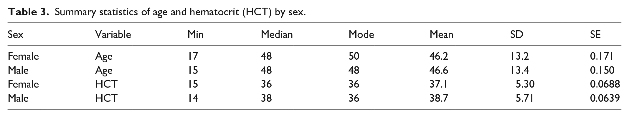
Table 4 illustrates the frequencies and percentages of hematocrit levels of the patients who received renal grafts according to sex, cardiac type, and rejection status. Among the 1160 patients, 43% were females, whereas 57% were males. Among these patients, 18% experienced cardiovascular problems during the years preceding transplantation, while 82% did not experience these problems. In addition, 32% of the patients experienced symptoms of graft rejection during the first 3 months after transplantation, whereas 68% of the patients did not.

Table 4.

Frequencies and percentages of hematocrit levels by covariates.

Statistics of hematocrit levels	Gender		Cardio		Reject
	Female	Male	Yes	No	Yes	No
Frequency	494	666	207	953	367	793
Percentage	42.59	57.41	17.84	82.16	31.64	68.36

Data exploration

Individual and mean profile plots

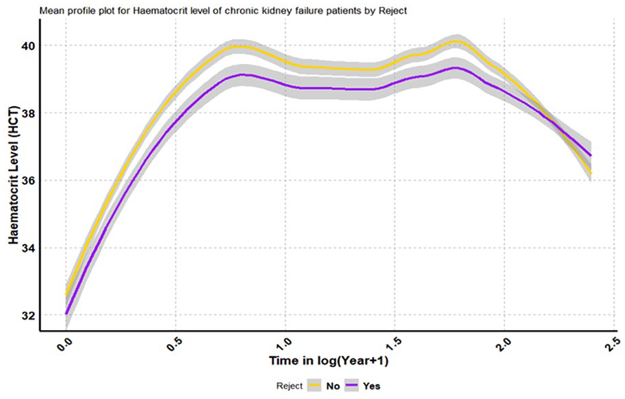
Figures 1 –6 present the overall individual plots, individual plots by category, overall mean plots, and mean plots by category. The charts show the changes in hematocrit levels over time. The overall mean profile and the mean profile for covariates appear to have a quadratic time trend. On average, male hematocrit levels appear to be higher than those of females over time. There appears to be no difference in average hematocrit levels over time between patients who experienced cardiovascular disease before transplantation and those who did not.

Figure 1.

Individual profile plot of the hematocrit levels of chronic kidney failure patients.

Figure 2.

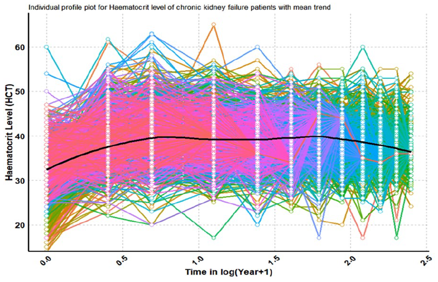
Individual profile plot of hematocrit levels in chronic kidney failure patients with a mean trend.

Figure 3.

Mean profile plot for the hematocrit level of chronic kidney failure patients.

Figure 4.

Mean profile plot for the hematocrit level of chronic kidney failure patients by sex.

Figure 5.

Mean profile plot for hematocrit levels in chronic kidney failure patients by cardio.

Figure 6.

Mean profile plot for the hematocrit level of chronic kidney failure patients by subject.

Patients who exhibit graft rejection signs within 3 months of transplantation appear to have lower average hematocrit levels than those who do not. As a result, the evolution of hematocrit levels appears to be governed by a quadratic temporal effect.

Figure 1 depicts an individual profile plot for the hematocrit level in chronic kidney failure patients. The graph depicts the hematocrit courses of individual patients over time, using a logarithm-transformed scale (log (year + 1)). The plot highlights significant variation in hematocrit levels among patients, reflecting variances in disease development, treatment response, and individual health conditions. Some patients’ hematocrit levels may be steady or increasing, indicating appropriate anemia therapy, whereas others show downward patterns, indicating deteriorating anemia as kidney function deteriorates. This heterogeneity emphasizes the importance of tailoring treatment strategies to specific patient demands. The plot emphasizes the importance of continual monitoring and appropriate interventions.

Overall, Figure 1 shows that the HCT of CKF patients decreased modestly with time. Throughout the follow-up, the heaviest HCT was typically rejected. This suggests that the variability of the measures at the start (baseline) of the follow-up was slightly lower than that at the end. Similarly, variance within groups occurs over time as the HCT decreases from year to year.

Figure 2 depicts an individual profile plot for the hematocrit level of chronic renal failure patients with a mean trend. The figure shows the hematocrit lines of individual patients over time, presented on a logarithmic converted scale (log (year + 1)), together with the overall mean trend. The plot shows high diversity in hematocrit levels among patients, which reflects changes in disease progression, treatment response, and individual health. The mean trend, depicted by a center line, demonstrates a gradual decrease in hematocrit levels over time, which is consistent with the progressive nature of CKD and its link to anemia. This heterogeneity emphasizes the importance of tailored treatment approaches that address individual patient needs, whereas the downward mean trend emphasizes the need for constant monitoring and appropriate treatments.

Figure 3 depicts the overall mean profile plot for the hematocrit level in chronic kidney failure patients. The general trend in hematocrit levels over time is displayed on a logarithmic scale. The plot depicts a gradual decrease in mean hematocrit levels over time, revealing the progressive nature of CKD and its impact on anemia. The logarithmic time scale makes it easier to observe the nonlinear progression of hematocrit levels, especially in the early phases after diagnosis or transplantation. This decreasing tendency emphasizes the importance of constant monitoring and prompt therapies, such as erythropoiesis-stimulating agents or iron supplements, in managing anemia and maintaining hematocrit levels within the desired range, which improves patient outcomes.

Figure 4 depicts the mean profile plot for hematocrit levels in chronic renal failure patients by sex. The graph depicts the longitudinal change in hematocrit levels over time, contrasting male and female patients. The X-axis indicates time on a logarithmic scale (log (year + 1)), which compensates for the nonlinear growth of hematocrit levels, whereas the Y-axis reflects average hematocrit levels. The graphic shows unique trajectories for males and females, suggesting both baseline differences and sex-specific reactions to CKD development or treatment. According to Vlahakos et al.,⁹ males have higher baseline hematocrit levels (45%–52%) than females do (37%–48%), and their trajectories are continuously greater. Hematocrit values may decrease over time in both sexes, indicating increasing anemia as kidney function deteriorates.

Males, on the other hand, may experience a delayed fall or a posttransplant increase, indicating PTE, which is defined by hematocrit levels greater than 51%. Females, who are more susceptible to anemia, may stabilize or gradually deteriorate. These sex-specific trends highlight the importance of customized therapies, such as PTE management in men and anemia treatment in women, in optimizing CKD patient outcomes.

Figure 5 depicts the hematocrit trajectories of individuals with and without a history of cardiovascular difficulties (cardio: yes/no) over time, shown on a logarithmic scale. Patients with cardiovascular problems (cardio: yes) may have lower baseline hematocrit levels because of the increased impact of cardiovascular illness on overall health. Over time, hematocrit levels in this population may decrease more quickly, suggesting the combined consequences of CKD and cardiovascular problems. Patients without cardiovascular problems (Cardio: no) may have more steady or higher hematocrit levels, indicating better general health and treatment response. These discrepancies underscore the impact of cardiovascular comorbidities on hematocrit evolution, emphasizing the importance of targeted therapies in patients with cardiovascular difficulties to manage anemia and enhance outcomes.

Figure 6 shows the differences in hematocrit trajectories between patients with and without rejection symptoms after transplantation (Reject: yes/no) across time on a logarithmic scale. Patients with rejection symptoms (Reject: yes) may have reduced hematocrit levels because of the immune-mediated response and accompanying comorbidities, which might worsen anemia. This group’s hematocrit levels may decrease more rapidly over time, reflecting the negative impact of rejection on renal function and overall health. Patients who do not experience rejection symptoms (Reject: no) may have more stable or higher hematocrit levels, indicating improved graft function and therapy response. These discrepancies highlight the necessity of regularly monitoring and controlling rejection symptoms to reduce their unfavorable impact on hematocrit levels and enhance posttransplant outcomes.

Aside from charting HCT across follow-up times in years, adding different subgroups on the same graph to demonstrate the link between the response variable HCT and the explanatory variables sex, cardio, and rejection over time is also important. Figures A.1–A.6 in the Supplemental materials present individual profile plots and the mean profile plots of HCT by sex, cardiological status, and rejection status, indicating that HCT levels initially increased across all categories of the variables, followed by a decline after certain follow-up time points

However, the slope for males appeared to be noticeably greater than the slope for females from baseline to the end of follow-up, indicating that the interaction effect did not exist because the slopes did not intersect.

Furthermore, Figures A.1–A.16 in Appendix A in Supplemental material show further graphical investigations, including diagnostic checking plots (Figures A.15–A.16 in Supplemental material).

Modeling classical simple LMs and simple linear mixed-effect model separately

Table 5 summarizes the results of classical simple linear regression models and simple linear mixed-effect models and compares the results of the models. Hence, the commonly used classical simple linear regression models for fixed effects, without considering random effects (Model A, Model B, and Model C), show that log-transformed year, age, and sex are each statistically significant predictors of HCT levels (p < 0.001). Among them, the simple linear regression model with the factor sex (Model C) explains the highest proportion of variance in HCT (R² = 1.90%), followed by log(year + 1; R² = 1.09%), and age (R² = 0.073%). However, the explained variances in all three models are minimal, signifying inadequate predictive power when fitted independently.

Table 5.

Classical simple linear regression and linear mixed-effects models for predicting hematocrit.

Model	Fixed effects	Estimate	SE	t-Value	p-Value	R ²	Adj. R²	F-statistic (df)	SE
Simple linear regression models
Model A	Intercept	36.8841	0.1044	353.28	<2e-16	0.0109	0.0108	153.5 (1, 13918)	5.561
Model A		Log (year + 1)	0.7736	0.0624	12.39	<2e-16
Model B	Intercept	36.3689	0.1715	212.04	<2e-16	0.00732	0.0072	102.5 (1, 13906)	5.572
Model B		Age	0.0360	0.0036	10.12	<2e-16
Model C	Intercept	37.1441	0.0719	516.39	<2e-16	0.01898	0.01891	269.3 (1, 13918)	5.538
Model C		Sex	1.5579	0.0949	16.41	<2e-16
Model	Fixed effects	Estimate	SE	t-Value	p-Value		AIC	BIC	LogLik
Simple or single predictor linear mixed-effect model
Model 1	Intercept	35.0567	0.1453	241.25	<0.001		82704.3	82772.1	−41343.1
Model 1	Log (year + 1)	1.0000	0.0781	12.81	<0.001		82704.3	82772.1	−41343.1
Model 2	Intercept	34.9783	0.2901	120.59	<0.001		82677.0	82744.9	−41329.5
Model 2	Age	0.0345	0.0060	5.75	<0.001		82677.0	82744.9	−41329.5
Model 3	Intercept	36.0371	0.1216	296.31	<0.001		82731.1	82799.0	−41356.6
Model 3	Factor (sex)1	1.1169	0.1605	6.96	<0.001		82731.1	82799.0	−41356.6
Component	Model 1		Model 2	Model 3
Variance–covariance structure (random effects + residual)
Sigma $(σ)$	4.29		5.00	5.08
$σ_{b_{0}}$	10.87		11.70	11.70
$σ_{b_{1}}$	4.37		4.37	4.37
$σ_{b_{2}}$	3.92		3.92	3.92
$ρ_{b_{0}, b_{1}}$	−0.470		−0.658	−0.677
$ρ_{b_{0}, b_{2}}$	0.318		0.527	0.548
ρb₁ ,b₂	−0.979		−0.981	−0.981

By contrast, the LMMs (Model 1, Model 2, and Model 3) account for random variation across within subjects and among subjects and give better model fit indicators with the lower values of AIC, BIC, and higher log-likelihood. Remarkably, the effect estimates remain consistent in direction with the classical simple linear regression models but slightly differ in magnitude. For example, the effect of sex is estimated as 1.56 in Model C and 1.12 in Model 3, while age and log(year + 1) show similar patterns across both model types.

Moreover, the linear mixed-effects models disclose considerable between-subject variability: the random intercept variance ( $σ_{b_{0}}$ ) ranges from 10.87 to 11.70, emphasizing that unobserved subject-level heterogeneity plays a significant role. This supports the use of mixed-effects modeling over simple linear regression for these data.

In summary, while classical simple linear regression recognizes important fixed effects, it captures little of the outcome variability. By contrast, the LMMs provide a substantially improved fit by accounting for the repeated measure data structure, making them more appropriate for modeling HCT in this context.

Model selections and comparisons

A primary goal of model selection is to choose the simplest model that provides the best fit to the observed data. There may be several choices concerning which fixed and random effects should be included in an LMM. There are also many possible choices of covariance structures for the D and $R_{i}$ matrices. The top-down strategy was used to select statistically significant covariates for the mixed-effect models with the outcome variable HCT. The models based only on fixed effects were selected with constant random effects first, and then, the significance of the random effects was also checked. The findings are displayed in Table 6 in different sections. First, time was considered years of follow-up, and then, the natural logarithms of years of follow-up were used. Hence, after passing through procedures, the model with natural logarithms of years of follow-up was selected with all variables and the quadratic slope random effect. Furthermore, the estimation methods with ML and REML were compared to determine that the ML estimation method was the most appropriate method for these data.

Table 6.

Model selections and comparisons.

Model	Models	ML			REML
Model	Models	AIC	BIC	LogLik	AIC	BIC	LogLik
Time = year and random intercept	Mod0	85425.7	85448.3	−42709.8	85428.6	85451.3	−42711.3
	Mod1	85424.3	85454.6	−42708.2	85434.3	85464.5	−42713.2
	Mod2	85326.1	85363.8	−42658.1	85344.2	85381.9	−42667.1
	Mod3	85252.7	85,298	−42620.4	85272.6	85317.8	−42630.3
	Mod4	85253.6	85306.4	−42619.9	85274.5	85327.3	−42630.2
	Mod5	85254.9	85315.2	−42619.4	85277.3	85337.6	−42630.6
Time = year and random slop	Mod0	84946.6	84984.5	−42468.4	84949.8	84987.5	−42469.9
	Mod1	84947.2	84992.4	−42467.6	84956.4	85001.6	−42472.2
	Mod2	84855.9	84908.7	−42420.9	84873.3	84926.1	−42429.6
	Mod3	84793.8	84854.1	−42388.9	84812.9	84873.3	−42398.5
	Mod4	84794.5	84862.3	−42388.2	84814.7	84882.6	−42398.4
	Mod5	84796.1	84871.5	−42388.0	84817.8	84893.2	−42398.9
Time = year and random quadratic slope	Mod0	84196.0	84256.4	−42090.0	84199.2	84259.6	−42091.6
	Mod1	84188.3	84256.2	−42085.2	84197.7	84265.6	−42089.9
	Mod2	84100.5	84175.9	−42040.2	84118.2	84193.6	−42049.1
	Mod3	84050.1	84133.0	−42014.0	84069.8	84152.7	−42023.9
	Mod4	84051.8	84142.3	−42013.9	84072.8	84163.3	−42024.4
	Mod5	84053.8	84151.8	−42013.9	84076.4	84174.5	−42025.2
Time = log (year) random intercept	Mod11	85226.3	85256.4	−42609.1	85233.2	85263.4	−42612.6
	Mod21	85127.9	85165.6	−42559.0	85143.0	85180.7	−42566.5
	Mod31	85054.5	85099.8	−42521.3	85071.4	85116.7	−42529.7
	Mod41	85274.5	85327.3	−42630.2	85274.5	85327.3	−42630.2
	Mod51	85056.7	85117.0		85076.1	85136.4	−42530.1
Time = log (year) and random slope	Mod11	84746.3	84791.6	−42367.2	84752.5	84797.8	−42370.3
	Mod21	84650.5	84703.3	−42318.3	84664.9	84717.7	−42325.5
	Mod31	84580.2	84640.5	−42282.1	84596.4	84656.7	−42290.2
	Mod41	84581.0	84648.9	−42281.5	84598.3	84666.1	−42290.1
	Mod51	84582.4	84657.8	−42281.2	84601.1	84676.5	−42290.6
Time = log (year) and random quadratic slope	Mod11	82704.3	82772.1	−41343.1	82710.7	82778.6	−41346.4
	Mod21	82606.6	82682	−41293.3	82621.5	82696.9	−41300.7
	Mod31	82561.5	82644.4	−41269.7	82578.2	82661.2	−41278.1
	Mod41	82562.4	82652.9	−41269.2	82580.4	82670.9	−41278.2
	Mod51	82564.4	82662.4	−41269.2	82584.1	82682.1	−41279.1
Model	DF	AIC	BIC	LogLik	Test	L.ratio	p-Value
Model selection among models with year or log (year) and different random effects
Mod1	8	85056.66	85116.99	−42520.33
Mod2	8	85254.87	85315.19	−42619.44
Mod3	10	84582.38	84657.79	−42281.19	2 vs 3	676.4859	<0.0001
Mod4	10	84796.07	84871.47	−42388.03
Mod5	13	82564.38	82662.41	−41269.19	4 vs 5	2237.6839	<0.0001
Mod6	13	84053.80	84151.82	−42013.90

In Table 6, the appropriate model for all the data was selected with all the covariates and the quadratic slope random effect model. Model selection from the null model to the full model was then conducted, and the findings are presented in Table 7.

Table 7.

Nested model selection of mixed-effect models HCT on log (year) and other predictors with quadratic slope random effects.

Model	AIC	BIC	logLik
Modbest1	82774.74	82835.07	−41379.37
Modbest2	82704.27	82772.14	−41343.14
Modbest3	82606.60	82682.00	−41293.30
Modbest4	82561.45	82644.39	−41269.72
Modbest5	82562.40	82652.88	−41269.20
Modbest6	82564.38	82662.41	−41269.19

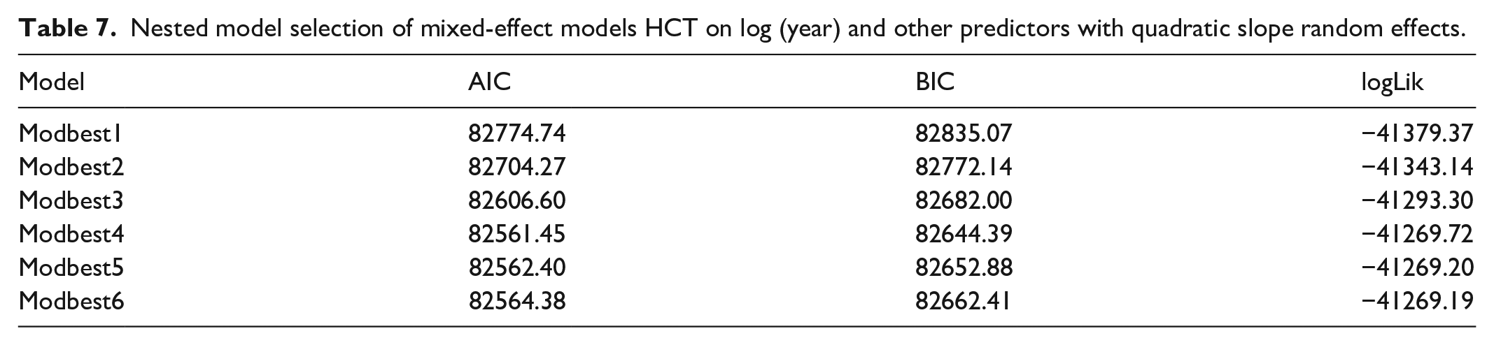
After all model selection procedures, the model with the covariates log(year + 1), age, sex, and cardio was rejected for fixed effects with a subject-specific random intercept and random slope, and the random quadratic slope for the HCT model was preferred, with relatively small values of AIC = 82561.45, BIC = 82644.39, and a log-likelihood ratio test with a p-value of <0.0001 for the model with the outcome variable HCT. The saturated model, which included the covariates cardio and reject in addition to the covariates that were included in the reduced model, was fitted and compared with the reduced model. However, the saturated model did not improve the model. Thus, statistically insignificant covariates, such as cardio and reject, were excluded from the final model. Finally, linear fixed effects and quadratic slopes for random effects improved the model, which is why they were also included in the model. In addition, the ML method, with a covariance structure of unstructured covariance structure with covariates log(year + 1), age, and sex for fixed effects with subject-specific random intercepts, random slopes, and quadratic random slopes, was preferred as the best-fit model that was appropriate for the entire dataset.

As illustrated in Table 7, the best-fit model for these data was the model with the predictor log(year + 1), age, and sex with quadratic slope random effects. Further details are presented in Table 7. After many model selection procedures, the best-fit model was the modeling HCT on log(year + 1), age, sex, and random effects with a quadratic slope.

The findings from the final model fixed effects results in Table 8 revealed that there was a significant linear (log(year + 1)) effect on the evolution of the hematocrit levels, which depended on the sex and age of the patients. In terms of sex, males tended to have greater changes in hematocrit levels than females did over time. However, high hematocrit levels are associated with increasing age. The findings show significant random intercept, random slope, and random quadratic slope effects in general. See Table 8 for more details.

Table 8.

Mixed-effect model for HCT on log (year + 1), age, sex, and random effects with a quadratic slope.

Effect type	Effect	Estimate (SE)	df	t-Value	p-Value	(1−α) 100% CI
Fixed effect	Intercept ( $β_{0}$ )	32.92 (0.319)	12,748	103.02	<0.0001	(32.283, 32.910)
	Log (year; $β_{1}$ )	0.9999 (0.078)	12,748	12.795	<0.0001	(0.847, 0.999)
	Age ( $β_{2}$ )	0.035 (0.006)	1156	5.879	<0.0001	(0.023, 0.046)
	Sex ( $β_{3}$ )	1.12 (0.158)	1156	7.075	<0.0001	(0.810, 1.431)
Random effect	Sigma ( $σ$ )	3.918			<0.0001	(3.866, 3.972)
	$σ_{b_{0}}$	4.182			<0.0001	(3.885, 4.502)
	$σ_{b_{1}}$	10.861			<0.0001	(10.299, 11.453)
	$σ_{b_{2}}$	4.372			<0.0001	(4.152, 4.603)
	$ρ_{b_{0}, b_{1}}$	−0.511			<0.0001	(−0.579, −0.436)
	$ρ_{b_{0}, b_{2}}$	0.363			<0.0001	(0.278,0.443)
	$ρ_{b_{1}, b_{2}}$	−0.979			<0.0001	−(0.982, −0.976)

Discussion

The analysis of longitudinal hematocrit levels in chronic kidney failure patients through a mixed-effects model has provided vital insights into the dynamic nature of hematocrit evolution. The significance of time (log(year + 1)), age, and sex for individual variability has arisen as fundamental factors impacting hematocrit trajectories among this patient cohort. Studies by Jha et al.,² Green et al.,³ and Smith et al.⁴ have emphasized the influence of time(log(year + 1)) on hematocrit levels, outlining the slow decline or irregular variations observed in chronic kidney failure. Our findings align with these observations, indicating the progressive influence on hematocrit trajectories within our patient population.

Furthermore, the influence of diverse age and sex modalities on hematocrit levels resonates with the findings of previous studies,^2–4 which elucidated the various responses to age and sex over time and their associations with different hematocrit trajectories. Our results highlight the differential effects of predictors on hematocrit levels and highlight the importance of tailored medical approaches for improved disease management. While addressing the unbalanced nature of our data within the mixed-effects model, we validated the study’s integrity, a point highlighted in the work of Jha et al.,² Green et al.,³ and Smith et al.,⁴ emphasizing the importance of appropriate data handling in longitudinal analyses. In conclusion, our study highlights the temporal influence of age and sex as major factors impacting hematocrit evolution in patients with chronic kidney failure over time. These findings echo the literature, suggesting the need for tailored treatments and personalized healthcare strategies for improved patient outcomes.

Potential factors that were found to be associated with the evolution of hematocrit levels were age and sex in the mixed-effect model. In the two-stage analysis, cardiovascular problems before renal transplant had a significant effect on hematocrit levels over time, which was not the case in the multivariate regression and linear mixed-effect models. In addition, experiencing rejection symptoms after transplantation had a significant quadratic random effect on hematocrit levels.

For the random effects, a linear mixed model revealed that HCT was positively correlated with age and sex throughout the follow-up period. This implies that patients who start with low hematocrit levels tend to have a greater increase over time. However, the correlation between the random effects in the linear mixed model was greater than that observed in the two-stage model analysis.

Overall, the results of this study revealed that sex and age have significant time effects on the evolution of hematocrit levels in renal transplant patients. The results showed that men are more likely to have high hematocrit values than females after a renal transplant. This finding coincides with results from other studies that revealed that men have higher hematocrit values than women.⁹ According to the literature, the normal ranges of hematocrit levels differ among males and females, with females having a lower range (45%–52% for men and 37%–48% for women)¹³; this finding coincides with our findings. However, these demarcations were not considered in the analysis. In addition, hematocrit levels in renal patients tend to increase with increasing age after transplantation. Older patients at transplant tend to have a greater increase in hematocrit levels over time. This difference might be attributed to the fact that the linear mixed model analysis models for both within- and between-subject variability, whereas the multiple linear regression model ignores between-subject variability.

Furthermore, cardiovascular problems before renal transplantation and rejection symptoms after transplantation had no significant effect on hematocrit levels in renal transplant patients according to the multivariate regression and linear mixed models. However, according to Winterbottom,⁵ these are some of the potential factors that affect the quality of life of renal patients and affect the levels of hematocrit in renal transplant patients. Thus, the results from this study might be attributed to the fact that only a few patients in the study experienced these problems (approximately 17% for cardiovascular disease and 31% for rejection), which requires further investigation.

The differences in the results might be attributed to the fact that the three analyses differ in the way they model the data. For example, the multivariate regression model addresses the variability within subjects. This implies that it ignores the variability between the subjects. However, two-stage analysis in some way solves the drawbacks encountered by multivariate regression models, which also address the variability between the subjects. Although two-stage analysis in some way solves the drawbacks of the multivariate regression model, it has its drawbacks, as it leads to a loss of information and introduces variability. However, the linear mixed model addresses the drawbacks encountered by the multivariate regression model and two-stage model by combining the two-stage models into one model, which results in more efficient and precise estimates of the regression coefficients.

Finally, this article considered the limited source of variables in the data and stuck to the few available predictors, including baseline age, sex (male = 1, female = 0), experience with cardiovascular problems during the year preceding the transplantation (Cardio: yes = 1, no = 0), and rejection symptoms during the first 3 months after the transplantation (Reject: yes = 1, no = 0), and the follow-up time in years. Because of these limitations, the manuscript has been developed based on the few available and statistically significant predictors, namely, baseline age, sex, and follow-up time in years. This study is limited in conducting a formal sample size determination procedure, because the researchers used secondary data and have not enough information on how the data source owners had determined the sample size for their study. Therefore, the manuscript was written based on all existing data from the secondary source.

Conclusion and recommendations

Conclusion

This longitudinal study was conducted to investigate the evolution of hematocrit levels in renal transplant patients over time and to assess the potential factors that might significantly affect this evolution. Different statistical methods, which involve linear mixed model approaches, have been employed to address scientific questions. The results of the mixed-effect model revealed that time or the natural logarithm of years of follow-up had a significant effect on the evolution of hematocrit levels in renal patients, and this evolution followed a quadratic slope random effect.

This research clarifies the complicated and diverse longitudinal evolution of hematocrit levels in chronic kidney failure patients through a vigorous and robust mixed-effects model. Findings underscore the fundamental roles of time (log(year + 1)), age, sex, and the noticeable individual variability among patients. The study’s fruitful handling of unbalanced longitudinal data adds validity and robustness to the findings, enhancing the understanding of hematocrit trajectories in the context of chronic kidney failure management.

In conclusion, time (log(years)) has a significant effect on the evolution of hematocrit levels in renal transplant patients. The study revealed that evolution varies according to sex and age. With age, it was observed that hematocrit levels tend to increase over time with increasing age after renal transplantation. Thus, older people tend to have greater increases in hematocrit levels than younger people do. On the other hand, males tend to have higher hematocrit levels over time than females do. Moreover, cardiovascular problems before renal transplantation and rejection symptoms after renal transplantation do not significantly affect the evolution of hematocrit levels over time in renal patients. Furthermore, patients who start with low hematocrit values tend to have a greater increase over time.

Recommendations

The results of this study indicate that the age of the patients is one of the main factors influencing their hematocrit levels. However, this increase in hematocrit levels in patients should be controlled to stay safe. Therefore, the government, health workers and professionals, and generally all stakeholders should follow patients and take responsibility for taking appropriate medicine or taking measurements to achieve normal levels (controlled levels) of hematocrit in patients.

These patients should be aware of all possible behaviors and controlling mechanisms of the disease. Patients should follow all the health professionals’ advice and then take all possible measurements to normalize their hematocrit levels (the normal hematocrit levels are 36%–48% for females and 40%–48% for males). All these can be done by following all the advice of the respective bodies, by balancing diets, etc. Respected bodies should teach people, especially health professionals and health workers, about such diseases.

The findings of this study strongly suggest that continued monitoring of hematocrit levels can serve as a reliable marker for long-term patient health outcomes in patients with chronic kidney failure.

The study’s implications further lead to recommendations for improved patient care and direct future research toward a more comprehensive understanding of hematocrit trajectories in this population.

Supplemental Material

sj-docx-1-smo-10.1177_20503121251360864 – Supplemental material for A mixed-effect model for the evolution of unbalanced longitudinal hematocrit levels in chronic kidney failure patients

Supplemental material, sj-docx-1-smo-10.1177_20503121251360864 for A mixed-effect model for the evolution of unbalanced longitudinal hematocrit levels in chronic kidney failure patients by Yemane Hailu Fissuh, Getachew Beyene Nega and Azmera Hailay in SAGE Open Medicine

Footnotes

Acknowledgements

The authors would like to express heartfelt gratitude to Mekelle University, Mekelle, Tigray, Ethiopia, for its partial funding grant from the graduate student grant fund and Mr. Mehari Gebre Teklezgi (meharistat@gmail.com) for providing permission to use his first-hand real data.

ORCID iD

Yemane Hailu Fissuh

Ethical considerations

This is to confirm that the previous researcher we acknowledged in this article and co-researchers have ethical approval from the research ethics approval committee, which is called the Institutional Review Board (IRB) of Hasselt University. It was confirmed that the IRB also approved the dataset for public utilization without personal, household identification. We have received the secondary data from the first owner and utilized this dataset for study purposes only.

Consent to participate

It was confirmed that the previous researchers who owned the first source of this data had carried out all the procedures in accordance with the relevant guidelines and regulations. It was also confirmed that the verbal full consent from the participants was obtained, verbal consent was used because the data were collected immediately by asking each participant for their consent, whereas written consent was not applicable. Therefore, the privacy of the participants was kept anonymous.

Author contributions

YHF conceptualized a proposal, conceptualized the methodology, organized the data set for analysis, and supported analysis via R programming. Furthermore, YHF supported the analysis and interpretation of the results, refined and organized the final research paper as supervisor of a master’s thesis at Mekelle University, extracted the research article from the whole thesis work, refined and prepared for publication, checked language and grammar errors, and finally acted as the corresponding author for submission. The corresponding author cross-checks many things, including author’s consent, conflicts of interest, and research ethics. GBN conceptualized the study, developed the research proposal, wrote the research, conceptualized the methodology, obtained the data, analyzed, conceptualized, interpreted, and organized the final research paper, which was submitted to Mekelle University for partial fulfillment of the Master of Science in Biostatistics. AH conceptualized the research paper and contributed to the editing, refining, writing, and organization of the thesis work as a co-supervisor of the thesis at Mekelle University. All the authors read and approved the final manuscript.

Funding

The author(s) disclosed receipt of the following financial support for the research, authorship, and/or publication of this article: This study had no formal fund, however, partially was supported from internal grant of Mekelle University, Mekelle Tigray, Ethiopia.

Declaration of conflicting interests

The author(s) declared no potential conflicts of interest with respect to the research, authorship, and/or publication of this article.

Data availability statement

The data were obtained upon a friendly sharing request through email from the first-hand data owner, Mehari Gebre Teklezgi (meharistat@gmail.com). Therefore, anyone who wants to use these data should kindly request it from Mehari Gebre Teklezgi at meharistat@gmail.com.

Supplemental material

Supplemental material for this article is available online.

References

Chen

Knicely

Grams

ME.

Chronic kidney disease diagnosis and management: a review. JAMA 2019; 322(13): 1294–1304.

Jha

Garcia-Garcia

Iseki

, et al. Chronic kidney disease: global dimension and perspectives. Lancet 2013; 382(9888): 260–272.

Green

, et al. Longitudinal modeling of hematocrit levels in chronic kidney disease under mixed effect models. J Nephrol 2020.

Smith

, et al. Statistical approaches for analyzing unbalanced longitudinal data in renal research. Kidney Int Rep 2021; 6(3): 698–705.

Winterbottom

A cross-sectional, correlational survey to explore the relationship between Renal Association biochemical and haematological markers and health-related quality of life in patients receiving haemodialysis in the North West of England. Doctoral Dissertation, University of Manchester, Manchester, UK, 2015.

Pan

Han

, et al. Association between hemoglobin and chronic kidney disease progression: a secondary analysis of a prospective cohort study in Japanese patients. BMC Nephrol 2022; 23: 295.

Hsu

C-Y

Vittinghoff

Lin

, et al. The incidence of end-stage renal disease is increasing faster than the prevalence of chronic renal insufficiency. Ann Intern Med 2004; 141: 95–101.

Teklezgi

Asres

Matope

, et al. Modeling the progression of haematocrit level over time. J Stat Theory Appl 2024; 23; 315–328.

Vlahakos

Marathias

Agroyannis

, et al. Posttransplant erythrocytosis. Kidney Int 2003; 63(4): 1187–1194.

10.

Fung

Haghamad

Montgomery

, et al. A retrospective multi-site examination of chronic kidney disease using longitudinal laboratory results and metadata to identify clinical and financial risk. BMC Nephrol 2024; 25: 447.

11.

Silveira

LTYD

Ferreira

Patino

CM.

Mixed-effects model: a useful statistical tool for longitudinal and cluster studies. J Bras Pneumol 2023; 49(2): e20230137.

12.

Vonesh

Tighiouart

Ying

, et al. Mixed-effects models for slope-based endpoints in clinical trials of chronic kidney disease. Stat Med 2019; 38(22): 4218–4239.

13.

Shiel

. Hematocrit, http://www.medicinenet.com/hematocrit/article.htm (2015, accessed 26 October 2016).

14.

Zoccali

Mallamaci

Adamczak

, et al. Cardiovascular complications in chronic kidney disease: a review from the European Renal and Cardiovascular Medicine Working Group of the European Renal Association. Cardiovasc Res 2023; 119(11): 2017–2032.

15.

Liao

Kao

Chang

, et al. An approach for personalized dynamic assessment of chronic kidney disease progression using joint model. Biomedicines 2024; 12: 622.

16.

Senel

Erken

Ozturk

, et al. Evaluation of platelet indices in chronic kidney disease. Interdiscip Med J 2024; 15(52): 72–79.

17.

Alagoz

Dincer

Eren

, et al. Prevalence of anemia in predialysis chronic kidney disease: is the study center a significant factor? PLoS One 2020; 15(4): e0230980.

18.

Gasparini

Abrams

Barrett

, et al. Mixed-effects models for health care longitudinal data with an informative visiting process: a Monte Carlo simulation study. Stat Neerl 2019; 74(1): 5–23.

19.

Akaike

. Information theory and an extension of the maximum likelihood principle. In: Petrov

Csaki

(eds.) 2nd International symposium on information theory. Budapest: Akademiai Kiado, 1973, pp. 267–281

20.

Schwarz

Estimating the dimension of a model. Ann Stat 1978; 6(2): 461–464.

21.

Verbeke

Molenberghs

Linear mixed models for longitudinal data. New York, NY: Springer, 2000.

22.

Brady

Konkle

Alvarez

, et al. Visual long-term memory has a massive storage capacity for object details. Proc Natl Acad Sci U S A 2008; 105(38): 14325–14329.

23.

Avendaño

Pierce

Schabenberger

, et al. The spatial distribution of soybean cyst nematode in relation to soil texture and soil map unit. Agron J 2004; 96(1): 181–194.

Supplementary Material

Please find the following supplemental material available below.

For Open Access articles published under a Creative Commons License, all supplemental material carries the same license as the article it is associated with.

For non-Open Access articles published, all supplemental material carries a non-exclusive license, and permission requests for re-use of supplemental material or any part of supplemental material shall be sent directly to the copyright owner as specified in the copyright notice associated with the article.

0.00 MB

3.08 MB