Sage Journals: Discover world-class research

Abstract

Transfer learning offers the potential to increase the utility of obtained data and improve predictive model performance in a new domain, particularly useful in an environment where data is expensive to obtain such as in a blast engineering context. A successful application in this respect will improve existing surrogate modelling approaches to allow for holistic and efficient strategies to protect people and structures subjected to the effects of an explosion. This paper presents a novel application of transfer learning for the prediction of peak specific impulse where we demonstrate that previous knowledge learned when modelling spherical charges can be transferred to provide a performance benefit when modelling cylindrical charges. To evaluate the influence of transfer learning, two artificial neural network architectures were stress tested for three levels of random data removal: the first model (NN) did not implement transfer learning whilst the second model (TNN) did by including a bolt-on network to a previously published NN model trained on the spherical dataset. It is shown the TNN consistently outperforms the NN, with this out-performance increasing as the proportion of data removed increases and showing statistically significant results for the low and high threshold with less variability in all cases. This paper indicates transfer learning applications can be used successfully with considerable benefit with respect to surrogate modelling in a blast engineering context.

Keywords

machine learning transfer learning blast computational fluid dynamics data-driven modelling

Introduction

Blast protection engineers are tasked with designing infrastructure such that it is resilient enough to withstand extreme loading. To perform the accurate appraisal of structures and protective systems subject to extreme near-field explosive blast loading, knowledge of both the distribution and the magnitude of loading are critical (Rigby et al., 2019b). Obtaining the loading information in this extreme near-field region, however, is particularly challenging. Experimental methods can be used to directly measure near-field reflected specific impulse and specific impulse distributions, for example, Hopkinson pressure bars (Edwards et al., 1992; Piehler et al., 2009; Rigby et al., 2015a; Cloete and Nurick, 2016; Tyas et al., 2016), impulse plugs (Huffington and Ewing, 1985; Nansteel et al., 2013) and flush-mounted pressure gauges (Aune et al., 2016). In this near-field region, the high magnitude of loading necessitates the use of robust support structures and protective housing for sensitive equipment. Additionally, the measurements themselves are highly variable owing to the presence of surface instabilities in the early stages of expansion of the detonation products (Rigby et al., 2020).

Therefore, it is not practical to develop a predictive approach based solely on physical testing. However, experimental data remains a fundamental requirement for validation of numerical modelling schemes. Computational fluid dynamics (CFD) and finite element (FE) approaches have been shown generally to provide good agreement with experimental data for near-field blast loading where it is available (Shin et al., 2014a; Rigby et al., 2018; Whittaker et al., 2019; Pannell et al., 2021). In spite of research into near-field blast loading currently being limited by a lack of well-controlled experimental validation data (Tyas, 2019), FE/CFD analyses can provide data at considerably higher spatial and temporal resolution than experimental studies and are therefore suitable tools with which to develop a refined predictive approach. However, physics-based models have a relatively high computational demand, and are unsuitable for probabilistic, risk-based analyses.

An appropriate technique is to use validated CFD analyses to create a dataset from which a surrogate model can be developed (Pannell et al., 2021). A fast-running surrogate model allows the analyst to rapidly obtain the loading information, within the parameters of the surrogate model, for a multitude of scenarios (that would otherwise be costly to ascertain) and is the first step towards a probabilistic mode of risk assessment. The preliminary surrogate model presented in Pannell et al. (2021) is an equation made of three separate terms and is suitable for a specific charge shape, type and range of scaled distances (spherical PE4 charges between 0.11 − 0.55 m/kg^1/3).

However, to increase the capabilities of the surrogate model proposed in Pannell et al. (2021), and therefore, the situations an analyst can simulate, a model that can handle additional complexity is required. Integrating data-driven methods with scientific theory is considered crucial in order to improve surrogate model performance whilst respecting natural laws (Reichstein et al., 2019). Pannell et al. (2022) investigated this by implementing a physics-based regularisation procedure when training a machine learning model through adding a monotonic loss constraint to the loss function.

Traditional data mining and machine learning algorithms provide predictions on future data using statistical models trained on previously collected labelled or unlabelled data (Pan and Yang, 2010; Ramon et al., 2007; Taylor and Stone, 2007). Many machine learning methods work under the assumption that the training and test data belong to the same distribution. When this distribution changes, most statistical models need to be re-trained on newly collected training data. Though some methods do exist that model non-stationary data where the ‘data-drift’ is parameterised and modelled, alternatively there are heuristic methods for continuous learning (Panoutsos and Mahfouf, 2008). In the context of blast protection engineering, obtaining data is considerably expensive in time and cost, and therefore, any method that increases the utility of this data is of paramount importance, as it would be in many other applications. In these cases it would be highly useful to reduce the need to re-collect training data, and therefore, knowledge transfer, or transfer learning, between task domains is highly desirable. Many examples exist where transfer learning can be beneficial such as web-document classification (Mahmud and Ray, 2007; Blitzer et al., 2008; Xing et al., 2007); sentiment classification (Li et al., 2009); image classification (Lee et al., 2007); WiFi localisation models (Yin et al., 2005; Raina et al., 2006; Pan et al., 2007, 2008; Zheng et al., 2008) and web-page translation (Ling et al., 2008). For an insight into the benefit transfer learning can explicitly bring over traditional machine learning approaches, see Table 5 in Pan and Yang (2010).

This paper presents a novel application of transfer learning for the prediction of near-field (0.2 − 0.5 m/kg^1/3) peak specific impulse distributions on a target surface from detonation of cylindrical charges of four different L/D ratios (0.2, 0.33, 0.5 and 1) of the same charge type (PE4). The overall aim of this paper is to establish the feasibility of implementing transfer learning to improve model performance in a new domain. This is achieved by transferring knowledge learned from a previously obtained dataset (Pannell et al., 2021) of near-field (0.11 − 0.55 m/kg^1/3) peak specific impulse distributions on a target surface produced from the detonation of spherical charges and incorporating this into the model that predicts peak specific impulse distributions produced by cylindrical charges in a similar scaled distance range (0.2 − 0.5 m/kg^1/3). The influence of transfer learning is evaluated by stress-testing two models: a neural network (NN) that does not implement transfer learning and a transfer neural network (TNN) that does implement transfer learning. The stress-tests consist of three different levels of data removal of the new cylindrical data. Discussion on dataset generation is provided in each case and assessments of the proposed models are presented. It is shown clearly that by implementing transfer learning, the need for new training data is drastically reduced.

Transfer learning

Transfer learning and domain adaptation refer to the situation where what has been learned in one scenario is exploited to improve generalisation in a second scenario. The inherent assumption is that the factors that influence variations in the first scenario also apply, to some level, to the second. In the real world, there are many clear examples of transfer learning. For example, one may find that learning to play the organ will facilitate learning the piano. The field of transfer learning is motivated by this awareness that people can apply previously learned knowledge intelligently when faced with a new problem and can solve it more quickly or with better solutions (Pan and Yang, 2010).

To aid understanding of transfer learning it is useful to have some formal notation and definitions. Firstly, the definitions of ‘domain’ and ‘task’. A domain, $D$ , consists of a feature space $X$ and a marginal probability distribution P(X), where $X = {x_{1}, \dots, x_{i}} \in X$ . Consider as an example the learning task of document classification where each term is taken as a binary feature, $X$ is the vector space for all terms, x_i is the ith term vector (corresponding to some documents) and X is a particular sample. It can generally be considered that if two domains are different, then they may have different feature spaces or marginal probability distributions (Pan and Yang, 2010).

Given a specific domain, $D = {X, P (X)}$ a task consists of two components: label space $Y$ and an objective predictive function $f : X \to Y$ and is denoted $T = {Y, f (\cdot)}$ . This predictive function is learned from the training data, pairs ${x_{i}, y_{i}}$ where x ∈ X and $y \in Y$ can be used to predict new labels f(x) from an instance x (Pan and Yang, 2010).

A definition of transfer learning is given as follows: ‘Given a source domain $D_{S}$ and learning task $T_{S}$ , a target domain $D_{T}$ and learning task $T_{T}$ , transfer learning aims to help improve the learning of the target predictive function f_T (·) in $D_{T}$ using the knowledge in $D_{S}$ and $T_{S}$ , where $D_{S} \neq D_{T}$ , or $T_{S} \neq T_{T}$ ’.

In the above definition, from Pan and Yang (2010), a domain is a pair $D = {X, P (X)}$ . So the condition that D_S ≠ D_T has the implication that X_S ≠ X_T or P_S(X) ≠ P_T(X). Likewise, a task is defined as a pair $T = {Y, P (Y | X)}$ , therefore the condition $T_{S} \neq T_{T}$ implies $Y_{S} \neq Y_{T}$ or $P (Y_{S} | X_{S}) \neq P (Y_{T} | X_{T})$ . If the source and target domains are the same $D_{S} = D_{T}$ , and their learning tasks are the same $T_{S} = T_{T}$ , the problem then becomes a classical machine learning problem.

There are considered to be three main research questions in the field of transfer learning: (1) what to transfer, (2) how to transfer and (3) when to transfer. ‘What to transfer’ is concerned with ascertaining which part of knowledge from the source can be transferred, and what may be useful knowledge to transfer for improving performance in the target domain or task. ‘How to transfer’ is concerned with choosing a learning algorithm that can transfer the knowledge from the source to the task, and ‘when to transfer’ considers when the transfer of knowledge should be implemented. An important point for consideration here is that it is equally useful in knowing when not to transfer as when to transfer. When transfer learning takes place and is harmful to performance in the target, it is referred to as negative transfer (Pan and Yang, 2010).

The overall objective of transfer learning is to take advantage of knowledge from the source domain $(D_{S})$ , and use this to improve performance when learning, or making predictions in the target domain $(D_{T})$ (Goodfellow et al., 2016). There are clear advantages to allowing more accurate predictions in the target domain, but a unique benefit to transfer learning is that accuracy of predictions can be high, even when data is sparse or severely limited (in $D_{S}$ ). This has the practical benefit that gathering new data is less important and there can be substantial savings in cost and time. For an extensive overview of advancements in transfer learning across a wide range of settings and implementations, see Pan and Yang (2010).

Modelling charge shape effects

Mesh sensitivity and model validation

The datasets used in this paper were generated from CFD simulations using Apollo Blastsimulator, a specialised CFD software dedicated to the simulation of detonations, blast waves and gas dynamics. Apollo solves the conservation equations for transient flows of inviscid, chemically reacting or inert gas mixtures. Apollo applies a finite-volume method with explicit time integration and uses a particular Reimann solver which efficiently copes with the extreme conditions present. Full second-order accuracy is achieved via a tri-linear reconstruction of cell-centred conservative variables (Fraunhofer EMI, 2018).

Prior to validating Apollo results against experimental data, a mesh sensitivity study was conducted with the aims of determining the required element size to achieve convergence and identifying suitable combinations of zone length and resolution level for cylindrical explosives. The chosen model set-up modelled a centrally detonated 0.078 kg PE4 squat cylinder (L/D = 1/3) axially aligned at 168 mm clear stand-off (0.1774 m perpendicular distance from centre of charge to target) after Rigby et al. (2019b). Quarter-symmetry was used, with symmetry planes located in the directions orthogonal to the reflecting wall, originating at the centre of the charge. All other boundaries were outflow boundaries, as summarised in Figure 1. The domain size was 1.2 m × 1.2 m × 1.2 m and Apollo’s auto-staging procedure was used throughout.

Figure 1.

0.078 kg PE4 squat cylinder (L/D = 1/3): CFD model set-up.

Apollo’s in-built model parameters were used for PE4. The pressure-density-temperature relationship of the post-detonation explosive products is given by the Jones Wilkins Lee equation of state (Lee et al., 1968)

p (ρ, T) = C_{1} e^{- R_{1} ρ_{0} / ρ} + C_{2} e^{- R_{2} ρ_{0} / ρ} + ρ R T

(1)

where ρ and ρ₀ are density and initial density, R is a gas constant, and T absolute temperature. The constants C₁, C₂, R₁ and R₂ are assigned the values given in Table 1. The air is modelled as a thermally perfect gas, p = ρRT, such that under ambient conditions (288 K), ambient pressure is p = 101.3 kPa. Afterburn was modelled using the Klomfass Afterburning (KAB) model, and the Chapman–Jouguet detonation model was used in all cases. In all numerical simulations, the explosives were centrally detonated and the mass of the detonator was not included. A Savitzky–Golay filter (Savitzky and Golay, 1964) has been used to remove spurious oscillations induced by Apollo’s DMA (dynamic mesh adaption) procedure.

Table 1.

Equation of state information for the five newly studies charge compositions, including the previously studied PE4.

Charge type	Gas constant J/(kg.K)	Initial density (kg/m³)	C₁ (GPa)	C₂ (GPa)	R ₁	R ₂
PE4	365	1660	734.60	8.86	4.79	1.06

For each analysis, 150 gauges are linearly spaced along the target surface at angles of incidence between 0 and 60°, where angle of incidence is defined as the angle between the outward normal of the surface and the direct vector from the explosive charge to that point. Each gauge outputs pressure-time histories at that location, which are numerically integrated (with respect to time) in postprocessing to yield specific impulse-time histories. The maximum of each of these is taken to provide the distribution of peak specific impulse.

The results of the mesh sensitivity study are shown in Figure 2: the three sub-plots represent peak perpendicular specific impulse, area-integrated impulse (on a 100 cm² circular plate), and simulation time. Figure 3 presents the studied meshes compared to the experimental peak specific impulse distribution where it can be shown that a mesh with a S/cell length from 336 shows good agreement with experimental data and can be considered suitable. The CFD model with S/cell length of 336 was chosen for further analysis, with the overpressure-time histories and impulse-time histories compared with experimental data and presented in Figure 4 where good agreement between CFD and experimental data is shown.

Figure 2.

Mesh convergence study for 0.078 kg PE4 cylinder, Z = 0.415 m/kg^1/3, stand-off from charge centre = 0.1774 m, L/D = 1/3.

Figure 3.

Mesh sensitivity analysis - comparison of different CFD models with experimental data.

Figure 4.

Experimental validation of numerical overpressure and specific impulse histories for Z = 0.415 m/kg^1/3 at 0, 25 and 50 mm perpendicular distance from the target centre.

Dataset generation

The dataset for cylindrical charges was generated from CFD simulations using Apollo consisting of centrally detonated 100g cylinders of PE4 located at five linearly spaced scaled distance values between 0.2 − 0.5 m/kg^1/3. Scaled distance, Z, according to Hopkinson–Cranz scaling (Hopkinson, 1915; Cranz, 1926) is given by S/W^1/3, where S is stand-off distance, and W is the mass of explosive. Therefore, the cylinders had stand-off values between 0.09m–0.23 m from the centre of the charge to a target. The general modelling schematic for these analyses are demonstrated in Figure 5. Four different L/D ratios were chosen of 1/5, 1/3, 1/2 and 1, where L/D represents length/diameter ratio. The domain size was 2 m × 2 m × 2 m, with 100 mm zone length and resolution level 3, otherwise the models follow a similar set-up to that outlined previously in Sec. 3.1.

Figure 5.

Model schematic for dataset generation: S is perpendicular stand-off distance between cylindrical charge and reflecting surface, gauges were placed along the perpendicular length r.

In summary, there are 20 CFD models (representing the five different stand-off distances analysed for each of the four different L/D ratios) with 150 values of peak specific impulse recorded for each, resulting in a dataset of 3000 samples, these are considered alongside the 2700 samples used to train the spherical network in Pannell et al. (2022) (shown in Figure 6). There are three input features: scaled distance (X₁), angle of incidence (X₂) and L/D ratio (X₃) with the labelled values Y representing peak specific impulse. An example entry from this dataset is shown in Table 2, and an overview of the cylindrical datasets presented in Figure 7.

Figure 6.

Spherical CFD dataset for the spherical network in Pannell et al. (2022).

Table 2.

Example dataset information for cylindrical dataset.

X ₁	X ₂	X ₃	Y
Scaled distance (m/kg^1/3)	Angle of incidence	L/D ratio	Peak specific impulse (MPa.ms)
0.1	15	1	45.87

Figure 7.

Cylindrical CFD dataset. Filled contours of scaled specific peak impulse for (a) L/D = 0.2, (b) L/D = 0.33, (c) L/D = 0.5, (d) L/D = 1.

The variables X₁ and X₂ are minmax scaled across the entire dataset using the scaling functions from the spherical model in Pannell et al. (2022), whilst X₃ is left unchanged, and varies between 0.2–1. The vector of labels, Y, has a log-normal distribution and is scaled via a power transform using the method described in Yeo and Johnson (2000) and again uses the same scaling function that scaled the spherical dataset labels used in Pannell et al. (2022). The result of this data transformation in presented in Figure 8, and the transformation is applied prior to model training to allow for the knowledge transfer.

Figure 8.

Unscaled Y dataset (left) and the resulting power transform (right).

In Pannell (2022, Chapter 6) it was demonstrated that prior knowledge from PE4 spheres can be leveraged to improve performance modelling spheres of different explosive types (TNT, HMX, RDX, PETN, COMPB). The specific method of applying a charge shape effect component was suitable as this applied across different charge compositions, and could be captured in a single exponential term (as shown in Pannell et al. (2021)). This exponential term modelled the ‘normalised’ impulse, which we defined as dividing subsequent specific impulse values (for 0° < θ ≤ 60°) by the respective specific impulse value located at 0°. Figure 9 demonstrates why this would not be a suitable approach for cylinders, as the normalised impulse profiles for cylinders are significantly different to a sphere, meaning the spherical model is not suitable. Furthermore, the normalised profile for each L/D ratio cannot be reasonably approximated to be the same profile whilst additionally is not always monotonically decreasing, necessitating the use of a more complex model.

Figure 9.

Normalised peak specific impulse comparison for four different L/D ratios: (a) 1/5, (b) 1/3, (c) 1/2 and (d) 1. In each case there are five normalised impulse curves corresponding to each scaled distance sample modelled. Note that here, non-normalised epicentral specific impulses from the cylindrical charges are between 2 and 6 times greater than those from a spherical charge at equivalent scaled distance (Rigby et al., 2021).

Application of transfer learning

Network architecture study

To model charge shape effects with transfer learning, two alternative network architectures were compared using the Keras package with Tensorflow backend (Chollet et al., 2015). The first model (NN) is shown in Figure 10(a) and does not utilise any transfer learning. It is only trained on the cylindrical dataset and provides a benchmark to compare a transfer network (TNN) to. It consists of three input nodes, one hidden layer and one output layer and is fully connected. The number of epochs was set at 1000, with early stopping, where the patience value was set as 50 epochs to prevent over-fitting.

Figure 10.

Model architectures for (a) NN architecture, model trained with no transfer learning and (b) Transfer neural network (TNN). In the TNN the previously trained ‘Spherical model’ is used and an additional ‘bolt-on’ network is added to handle the additional L/D input. The output of the spherical model (i_s) and bolt-on network (i_c) are summed to produce the overall model output.

The TNN structure is shown schematically in Figure 10(b), it consists of a pre-trained spherical model that was trained on the spherical dataset and is the network produced in Pannell et al. (2022), and a ‘bolt-on’ network that handles the additional feature, X₃ (L/D). The output from both the spherical model and the bolt-on model are summed to provide an overall model output for the TNN. During model training, the spherical model is ‘frozen’ so that the parameters are not updated during back-propagation, and the only parameters that are updated are in the bolt-on network. This means the information that the pre-trained model contains is preserved. After the initial 1000 epochs training, the TNN is fine-tuned by un-freezing the spherical model, reducing the learning rate by an order of magnitude and training for 100 further epochs (with early-stopping implemented again). This allows any incremental improvements on the pre-trained features to be made. This process of transfer learning, specifically the fine-tuning stage, is based on that outlined in Chollet (2021, Chapter 5).

In both cases the activation functions for the hidden units were set as hyperbolic tangent, with layer weights initialised with the Glorot normal initialiser (Glorot and Bengio, 2010). The ‘Adam’ algorithm was chosen as the optimiser, a stochastic gradient descent method that is based on adaptive estimation of first-order and second-order moments. The dataset consists of all L/D ratios and K-fold cross-validation was implemented with five splits, following an initial data split of 25% data randomly removed (and these values were chosen heuristically). The batch size was set at 32.

A varying number of hidden units are examined ranging from 1 to 10 in increments of 1. The hidden units apply to the hidden layer in Figure 10(a) and the hidden layer in the bolt-on network in Figure 10(b). All networks contain one hidden layer. The results of these analyses are presented in Figure 11 where six separate sub-figures provide: mean absolute error (Figures 11(a) and 11(d)), mean squared error (Figures 11(b) and 11(e)) and coefficient of determination (Figures 11(c) and 11(f)) for the NN and TNN, respectively. For all analyses, the metrics are evaluated for the three separate data portions: train, validation and test data and all L/D ratios are considered in aggregate. If any large discrepancies occur between data portions (train, test or evaluate), this can be indicative of over-fitting issues. For the NN the global minimum mean MAE and MSE occur with 6 units in the hidden layer, suggesting that this capacity provides adequate predictive capability. For the TNN, a sufficient capacity is provided by six hidden units in the bolt-on sub-network. These two model architectures were taken forward for further modelling.

Figure 11.

Hyper-parameter configuration of NN (a, b, c) and TNN (d, e, f). Mean absolute error (a, d), mean squared error (b, e) and coefficient of determination (c, f). Error bars are standard deviation.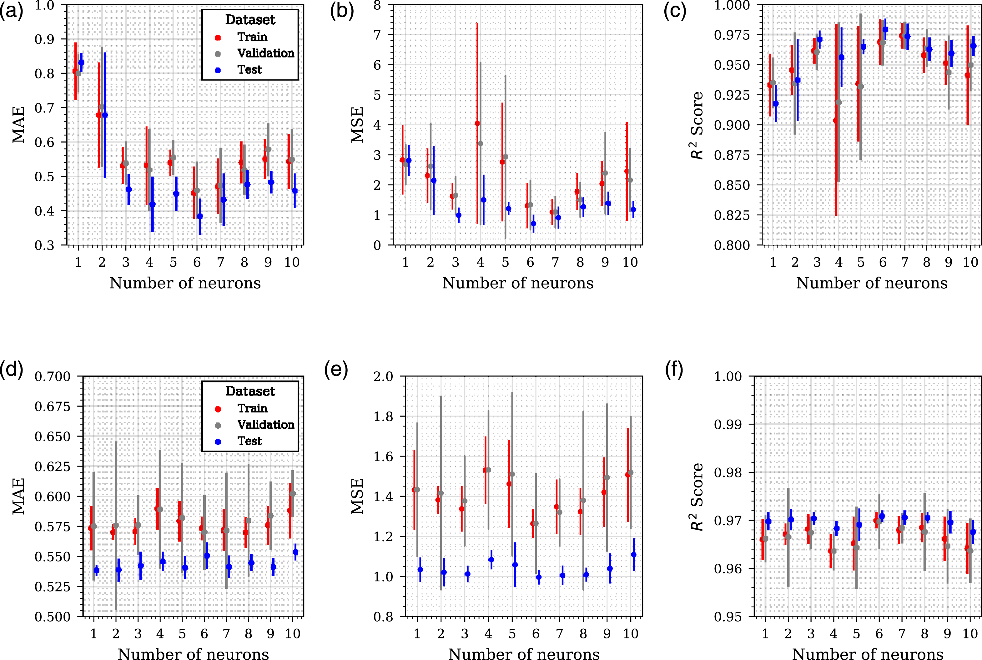

Stress-testing: Set-up

As previously discussed, obtaining data is expensive within a blast engineering context (and commonly other domains). A useful assessment for the utility of transfer learning would be how the models perform when data is increasingly limited; any model or modelling framework that would improve the performance in a low-data environment would be highly beneficial. To test this, the cylindrical dataset has been limited by three separate levels of random data removal: a low threshold representing 20% data removal, a medium threshold representing 55% data removal, and a high threshold representing 90% data removal. The effects of this data restriction on the dataset is shown in Figure 12.

Figure 12.

Distributions for (a) 20%, (b) 55% and (c) 90% random data removal. Each of the four plots in the right hand side represent a one of the four L/D ratios with a shaded pixel representing the presence of data. The features are scaled using the fitted scalers from the dataset of spherical data in Pannell et al. (2022).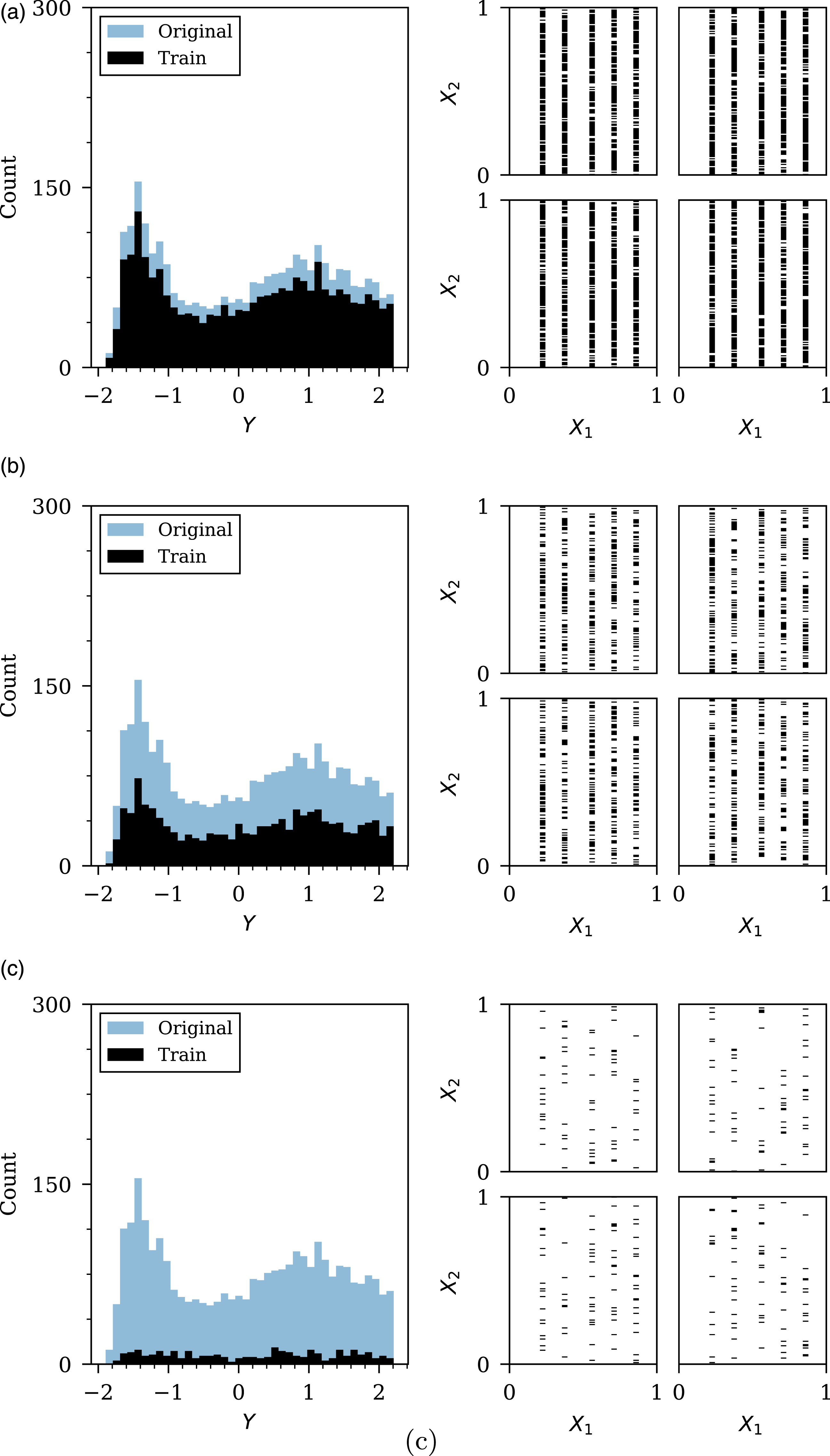

Stress-testing: Results

The modelling procedure follows that set out in Sec. 4.1, with the exception that the K-fold cross-validation procedure is repeated 3 times for five splits. The results of these analyses are shown in Figure 13, with sub-figures for each of the three assessment metrics: mean absolute error (Figure 13(a)), mean squared error (Figure 13(b)) and coefficient of determination (Figure 13(c)). The points plotted are mean values, whilst the error bars represent standard deviation. For the 90% removal case in Figure 13(c), the values for the NN have been omitted due to negative values, indicating the model performs arbitrarily worse than a constant model that always predicts the mean true value (which would give an R² of 0).

Figure 13.

Stress-test results from three data holdout proportions. The coefficient of determination values for the NN in the 0.9 data holdout case have been omitted due to negative values, indicating the model performs arbitrarily worse than a constant model that always predicts the mean true value.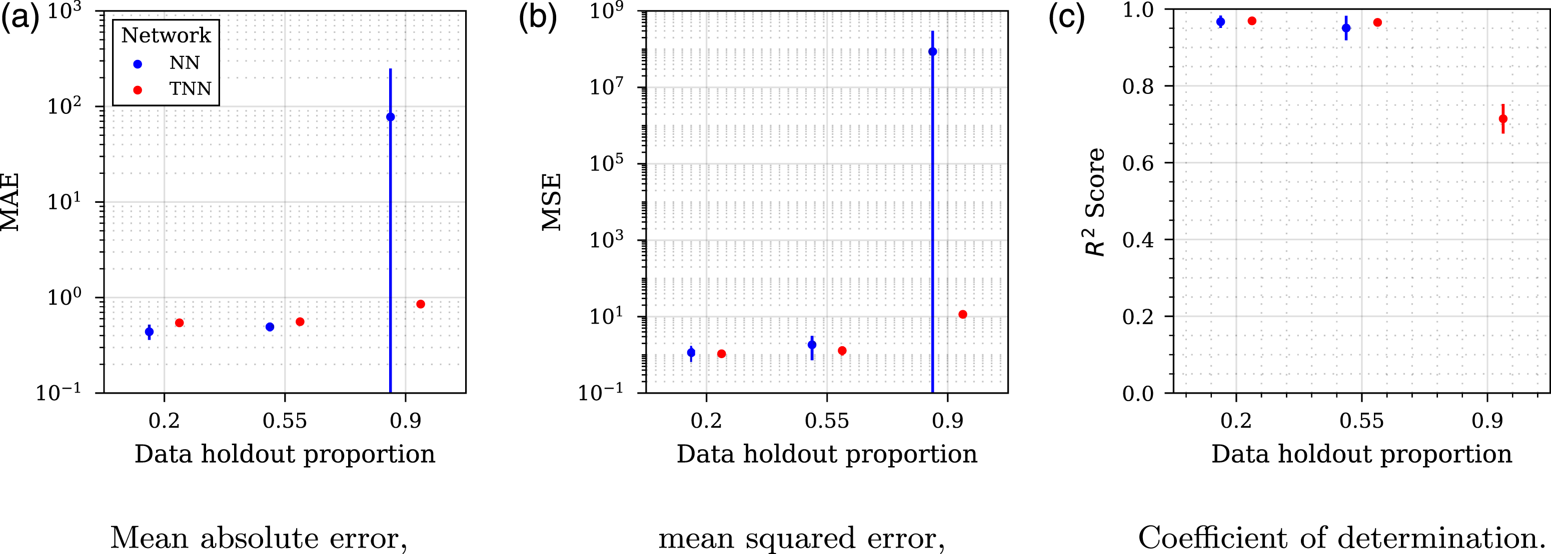

To better understand how each model is learning, a training history from the high threshold removal (90% data removal) case is presented in Figure 14 comparing the two different models NN and TNN. The TNN has been included as two separate parts in the legend, the initial training when the spherical model is frozen, followed by the ‘fine-tuning’, where the entire model can be updated.

Figure 14.

Training history for 90% data holdout of the two different networks (NN and TNN). ‘TNN-2’ represents the fine-tuning of the TNN.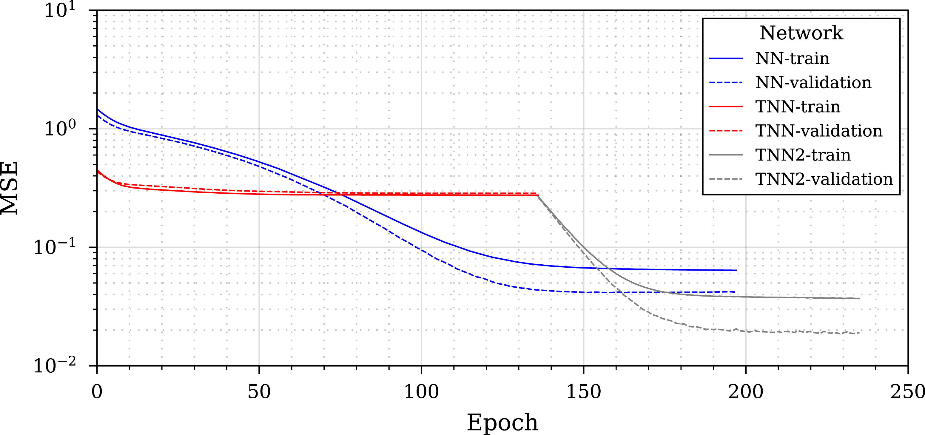

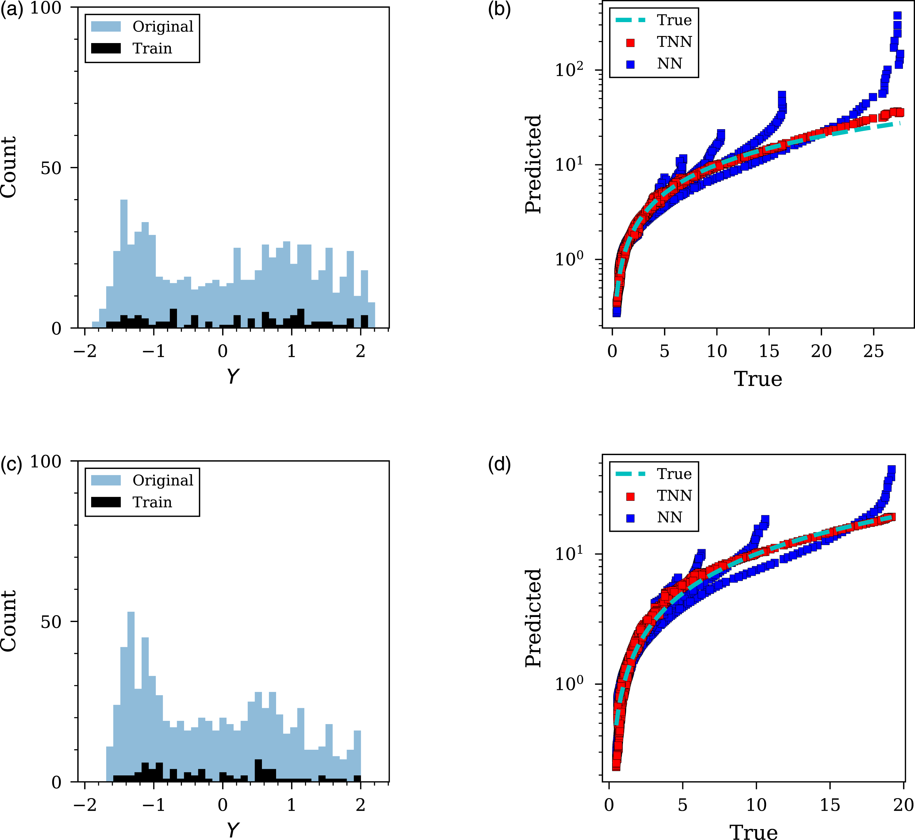
The critical case of 90% data removal was explored further and shown in Figures 15 and 16, representing each of the four L/D ratios. In each figure, the training and unseen data are presented alongside the predictions made for the entire unseen dataset. It can be seen in these Figures what information is available to each model and how it influences the accuracy of model predictions. Furthermore, the ‘true’ data (representing actual CFD values) has been included to aid the evaluation of the NN and TNN’s predictions due to the different axis scales.

Figure 15.

Stress-testing of 100g PE4 cylinder with 90% data removed. (a) and (c) histogram of original and training data for L/D =0.2 and 0.33, respectively; (b) and (d) predicted versus true unseen data for L/D =0.2 and 0.33, respectively. ‘True’ data (shown by the dashed blue line) represents actual CFD values and has been included to aid comparison due to the different axis scales.

Figure 16.

Stress-testing of 100g PE4 cylinder with 90% data removed. (a) and (c) histogram of original and training data for L/D =0.5 and 1, respectively; (b) and (d) predicted versus true unseen data for L/D =0.5 and 1, respectively. ‘True’ data (shown by the dashed blue line) represents actual CFD values and has been included to aid comparison due to the different axis scales.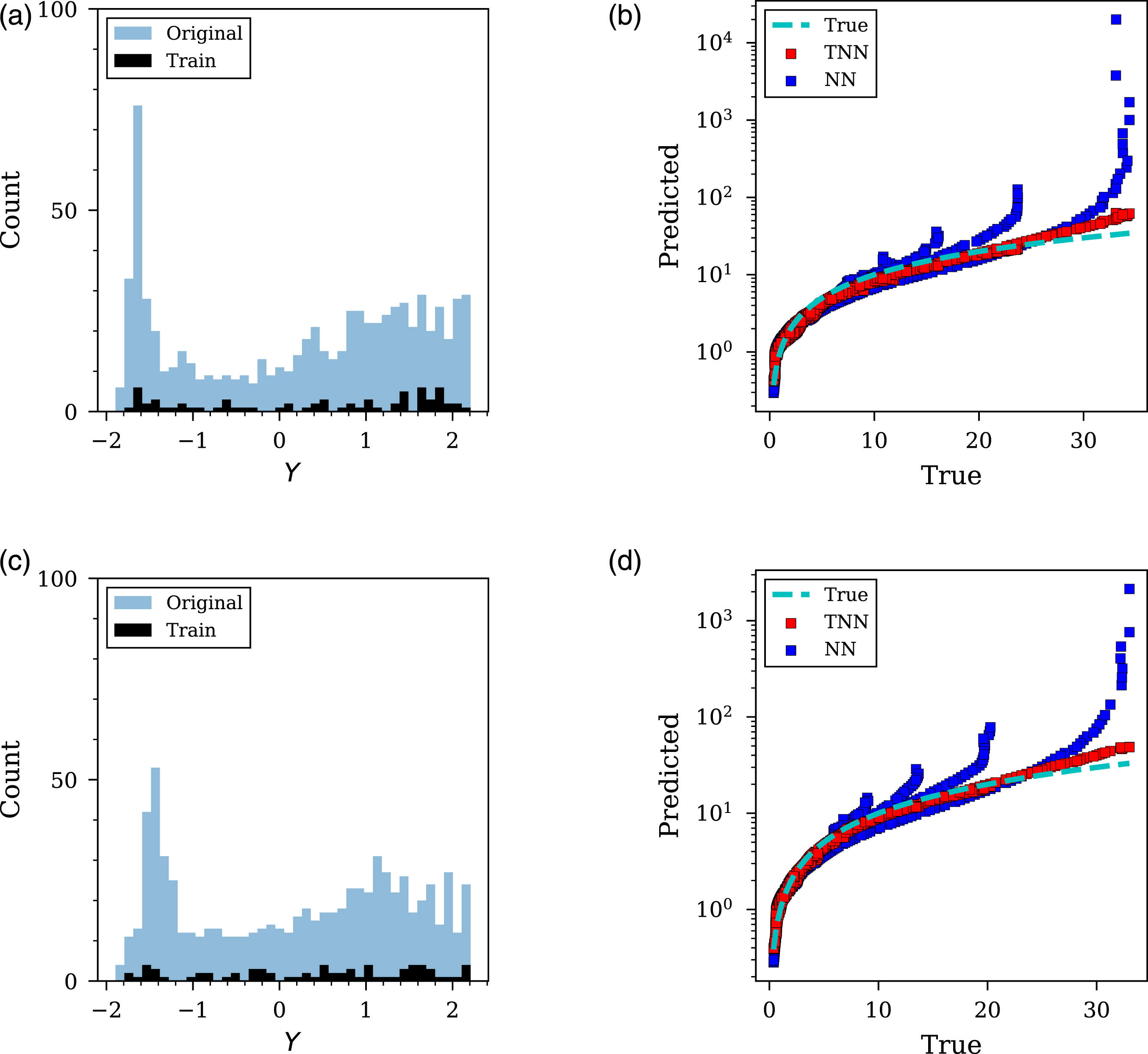

Discussion

The results from the stress-testing evaluation for the NN and TNN are compared in Table 3. To check the statistical significance of the results from each test, two-tailed Kolmogorov–Smirnov (KS) tests (Hodges, 1958) have been performance in each case. This is a two-tailed test to evaluate the hypothesis that both sets of independent samples are drawn from the same continuous distribution. In this analysis, it establishes if any performance premium is statistically significant.

Table 3.

Mean RMSE results from each stress-testing evaluation of NN and TNN models, with standard deviation given in brackets. RMSE values are from the unseen, test data. Entries in bold indicate a statistically significant difference (p < 0.10) from the Kolmogorov–Smirnov two-tailed test statistic (Hodges, 1958) for performance premium (two-tailed p-value).

Data holdout, %	Mean RMSE ± (SD.)
	NN	TNN
20	1.047 (±0.230)	1.033 (± 0.037)
55	1.314 (±0.335)	1.133 (±0.106)
90	3841.733 (±8458.127)	3.384 (± 0.212)

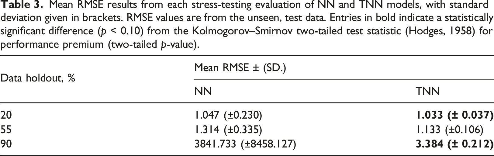
For every metric and for each data holdout proportion it can be seen that the TNN shows a performance premium over the NN, and this performance premium widens as the data holdout proportion increases. This performance premium is shown to be statistically significant for data holdout values of 20% and 90%. Since the performance premium widens as the proportion of data removed increases, it suggests that the transfer learning has more utility as data becomes increasingly limited. The TNN shows drastically less variability than the NN in all cases as shown by the considerably smaller standard deviation values.

A further insight into this performance premium can be seen in the training history from Figure 14. Initially it would appear that the NN is learning well, and there is a clear gap between the NN and TNN, until the TNN enters the fine-tuning stage. After the fine-tuning stage the TNN shows a clear performance premium over the NN and would appear to be a crucial element in the transfer learning implementation.

The stress-testing overview in Figures 15 and 16 further demonstrate the effectiveness of transfer learning. As shown, when predicting values at the minimum values of angle of incidence and scaled distance, the NN often over-predicts, quite drastically in some instances. This is demonstrated in Sub-figures 15b, 15d, 16b and 16d where the TNN remains closer to the ‘true’ line plotted and the NN diverges from this when predicting the maximum values. It suggests that the knowledge gained from the spherical dataset is useful in preventing such drastic over-predictions, even though there is considerable difference in charge shape.

These results are highly promising, particularly from an engineering perspective. It has been established that knowledge of the source domain $(D_{S})$ and task $(T_{S})$ can be used to provide more accurate predictions and improve learning in the target domain $(D_{T})$ and task $(T_{T})$ . In this instance the source domain is the spherical dataset and the target domain is the cylindrical dataset. The important practical implication of this finding can improve the efficiency of experimental design and improve the accuracy of predictive models in a blast engineering setting.

Summary

This paper presents a novel application of transfer learning for the prediction of peak specific impulse in a blast engineering setting. The implementation aimed to investigate if knowledge obtained when modelling spherical explosives could be used to improve the learning when modelling cylinders. An initial architecture study was completed for two separate network architectures to determine a model that had a sufficient capacity to model the cylindrical charges. The first model (NN) did not implement any transfer learning and was included as a benchmark for comparison; this network did not have knowledge of the spherical dataset. The second network (TNN) did implement transfer learning through incorporating the trained spherical model proposed in Pannell et al. (2022), with an additional ‘bolt-on’ network to handle the new L/D parameter. The models were stress tested for three levels of random data removal, where it is shown the TNN outperforms the NN for every level, with this out-performance increasing as the percentage of data removed increases and showing statistically significant results for the low and high threshold. The TNN also shows less variability in each case shown by the far smaller standard deviation values.

In a domain where data is expensive to obtain, a method is proposed here that improves the utility of data already obtained and demonstrates how this can be used when modelling a new, but related, domain within a blast engineering context. The implications of this research can directly affect how experiments are designed and will facilitate more accurate probabilistic-based approaches to experimental design and risk mitigation that encompass a more complex suite of scenarios than is capable presently.

Footnotes

Acknowledgements

J. J. Pannell gratefully acknowledges the financial support from the Engineering and Physical Sciences Research Council (EPSRC) Doctoral Training Partnership.

Declaration of conflicting interests

The author(s) declared no potential conflicts of interest with respect to the research, authorship, and/or publication of this article.

Funding

The author(s) disclosed receipt of the following financial support for the research, authorship, and/or publication of this article: Jordan J Pannell gratefully acknowledges the financial support from the Engineering and Physical Sciences Research Council (EPSRC) Doctoral Training Partnership.

ORCID iDs

Jordan James Pannell

Sam E Rigby

References

Aune

Fagerholt

Hauge

, et al. (2016) ‘Experimental study on the response of thin aluminium and steel plates subjected to airblast loading’, International Journal of Impact Engineering 90, 106–121.

Blitzer

Crammer

Kulesza

, et al. (2008) ‘Learning Bounds for Domain Adaptation’.

Chollet

(2021) Deep Learning with Python, Simon & Schuster.

Chollet

et al. (2015) ‘Keras’, https://keras.io

Cloete

Nurick

(2016), ‘Blast characterization using a ballistic pendulum with a centrally mounted Hopkinson bar’, International Journal of Protective Structures 7(3), 367–388.

Cranz

(1926), Lehrbuch der Basllistik, Springer, Berlin, Germany.

Edwards

Thomas

Milne

, et al. (1992) ‘Blast wave measurements close to explosive charges’, Shock Waves 2, 237–243.

Fraunhofer EMI (2018), APOLLO Blastsimulator Manual, Version: 2018.2, Fraunhofer Institute for High-Speed Dynamics, Ernst-Mach-Institut, Freiburg, Germany.

Glorot

Bengio

(2010), Understanding the difficulty of training deep feedforward neural networks, in Teh

Titterington

, eds ‘Proceedings of the Thirteenth International Conference on Artificial Intelligence and Statistics’, Vol. 9, Chia Laguna Resort, Sardinia, Italy, pp. 249–256.

10.

Goodfellow

Bengio

Courville

(2016), Deep Learning, Adaptive Computation and Machine Learning, The MIT Press, Cambridge, MA.

11.

Hodges

(1958) ‘The significance probability of the smirnov two-sample test’, Arkiv för Matematik 3(5), 469–486.

12.

Hopkinson

(1915), British Ordnance Board Minutes, 13565.

13.

Huffington

Ewing

(1985), Reflected Impulse Near Spherical Charges, BRL-TR-2678, Ballistic Research Laboratories, MD, USA.

14.

Lee

Hornig

Kury

(1968), Adiabatic Expansion of High Explosive Detonation Products, TID 4500-UCRL 50422, Lawrence Radiation Laboratory, University of California, CA, USA.

15.

Lee

S-I

Chatalbashev

Vickrey

, et al. (2007), Learning a meta-level prior for feature relevance from multiple related tasks, In ‘Proceedings of the 24th international conference on Machine learning’, pp. 489–496.

16.

Yang

Xue

(2009), Can movies and books collaborate? cross-domain collaborative filtering for sparsity reduction, In ‘Twenty-First international joint conference on artificial intelligence’, Citeseer.

17.

Ling

Xue

G-R

Dai

, et al. (2008), Can chinese web pages be classified with english data source? In ‘Proceedings of the 17th international conference on World Wide Web’, pp. 969–978.

18.

Mahmud

Ray

(2007), Transfer learning using kolmogorov complexity: Basic theory and empirical evaluations, Technical Report.

19.

Nansteel

Veldman

Chen

CC-T

, et al. (2013), ‘Impulse plug measurements of blast reflected impulse at close range’, Propellants, Explosives, Pyrotechnics 38(1), 120–128.

20.

Pan

Kwok

Yang

, et al. (2007), Adaptive localization in a dynamic wifi environment through multi-view learning, in ‘22nd AAAI Conference on Artificial Intelligence, AAAI-07 and the 19th Innovative Applications of Artificial Intelligence Conference’, IAAI-07, Vancouver, Canada, 22-26 July 2007, pp. 1108–1113.

21.

Pan

Shen

Yang

, et al. (2008), Transferring Localization Models across Space., in ‘AAAI’, pp. 1383–1388.

22.

Pan

Yang

(2010), ‘A survey on transfer learning’, IEEE Transactions on Knowledge and Data Engineering 22(10), 1345–1359.

23.

Pannell

(2022), Surrogate Modelling with Machine Learning for Blast Load Prediction, PhD thesis, University of Sheffield.

24.

Pannell

Panoutsos

Cooke

, et al. (2021), ‘Predicting specific impulse distributions for spherical explosives in the extreme near-field using a gaussian function’, International Journal of Protective Structures p. 12, 459.

25.

Pannell

Rigby

Panoutsos

(2022), ‘Physics-informed regularisation procedure in neural networks: an application in blast protection engineering’, International Journal of Protective Structures. Advanced online publication. doi: 10.1177/20414196211073501

26.

Panoutsos

Mahfouf

(2008), An incremental learning structure using granular computing and model fusion with application to materials processing, In ‘Intelligent Techniques and Tools for Novel System Architectures’, Springer, pp. 139–153.

27.

Piehler

Birk

Benjamin

, et al. (2009), Near-Field Impulse Loading Measurement Techniques for Evaluating Explosive Blast, ARL-RP-235, Army Research Laboratory, MD, USA.

28.

Raina

Koller

(2006), Constructing informative priors using transfer learning, In ‘Proceedings of the 23rd international conference on Machine learning’, pp. 713–720.

29.

Ramon

Driessens

Croonenborghs

(2007), Transfer learning in reinforcement learning problems through partial policy recycling, In ‘European Conference on Machine Learning’, Springer, pp. 699–707.

30.

Reichstein

Camps-Valls

Stevens

, et al. (2019), ‘Deep learning and process understanding for data-driven Earth system science’, Nature 566(7743), 195–204.

31.

Rigby

Akintaro

Fuller

, et al. (2019b), ‘Predicting the response of plates subjected to near-field explosions using an energy equivalent impulse’, International Journal of Impact Engineering 128, 24–36.

32.

Rigby

Fuller

Tyas

(2018), Validation of near-field blast loading in LS-DYNA, In ‘5th International Conference on Protective Structures (ICPS5), Poznan, Poland’.

33.

Rigby

Knighton

Clarke

, et al. (2020), ‘Reflected near-field blast pressure measurements using high speed video’, Experimental Mechanics 60(7), 875–888.

34.

Rigby

Osborne

Langdon

, et al. (2021), ‘Spherical equivalence of cylindrical explosives: Effect of charge shape on deflection of blast-loaded plates’, International Journal of Impact Engineering 155, 103892.

35.

Rigby

Tyas

Clarke

, et al. (2015a), ‘Observations from Preliminary Experiments on Spatial and Temporal Pressure Measurements from Near-Field Free Air Explosions’, International Journal of Protective Structures 6(2), 175–190.

36.

Savitzky

Golay

MJE

(1964), ‘Smoothing and differentiation of data by simplified least squares procedures’, Analytical Chemistry 36(8), 1627–1639.

37.

Shin

ttaker

Cormie

, et al. (2014a), ‘Numerical modeling of close-in detonations of high explosives’, Engineering Structures 81, 88–97.

38.

Taylor

Stone

(2007), Cross-domain transfer for reinforcement learning, In ‘Proceedings of the 24th international conference on Machine learning’, pp. 879–886.

39.

Tyas

(2019), Blast loading from high explosive detonation: what we know and what we don’t know, In ‘13th International Conference on Shock and Impact Loads on Structures’, Guangzhou, China.

40.

Tyas

Reay

Fay

, et al. (2016), ‘Experimental studies of the effect of rapid afterburn on shock development of near-field explosions’, International Journal of Protective Structures 7(3), 456–465.

41.

Whittaker

Klomfass

Softley

, et al. (2019), Comparison of numerical analysis with output from precision diagnostics during near-field blast evaluation, In ‘18th International Symposium on Interaction of the Effects of Munitions with Structures (ISIEMS18), Panama City Beach, FL, USA’.

42.

Xing

Dai

Xue

G-R

, et al. (2007), Bridged refinement for transfer learning, In ‘European Conference on Principles of Data Mining and Knowledge Discovery’, Springer, pp. 324–335.

43.

Yeo

I-K

Johnson

(2000), ‘A new family of power transformations to improve normality or symmetry’, Biometrika 87(4), 954–959.

44.

Yin

Yang

(2005), Adaptive temporal radio maps for indoor location estimation, In ‘Third IEEE international conference on pervasive computing and communications’, IEEE, pp. 85–94.

45.

Zheng

Xiang

Yang

, et al. (2008), Transferring localization models over time. In ‘AAAI’, Vol. 2008, pp. 1421–1426.

Application of transfer learning for the prediction of blast impulse

Abstract

Keywords

Introduction

Transfer learning

Modelling charge shape effects

Mesh sensitivity and model validation

Dataset generation

Application of transfer learning

Network architecture study

Stress-testing: Set-up

Stress-testing: Results

Discussion

Summary

Footnotes

Acknowledgements

Declaration of conflicting interests

Funding

ORCID iDs

References