Sage Journals: Discover world-class research

Abstract

Machine learning offers the potential to enable probabilistic-based approaches to engineering design and risk mitigation. Application of such approaches in the field of blast protection engineering would allow for holistic and efficient strategies to protect people and structures subjected to the effects of an explosion. To achieve this, fast-running engineering models that provide accurate predictions of blast loading are required. This paper presents a novel application of a physics-guided regularisation procedure that enhances the generalisation ability of a neural network (PGNN) by implementing monotonic loss constraints to the objective function due to specialist prior knowledge of the problem domain. The PGNN is developed for prediction of specific impulse loading distributions on a rigid target following close-in detonation of a spherical mass of high explosive. The results are compared to those from a traditional neural network (NN) architecture and stress-tested through various data holdout approaches to evaluate its generalisation ability. In total the results show five statistically significant performance premiums, with four of these being achieved by the PGNN. This indicates that the proposed methodology can be used to improve the accuracy and physical consistency of machine learning approaches for blast load prediction.

Keywords

Machine learning physics-guided neural network deep learning blast computational fluid dynamics data-driven modelling

Introduction

Initiation of an explosive charge rapidly converts the material into high-energy gaseous products of detonation. This gas initially occupies the same volume as the explosive but at pressures, densities and temperatures orders of magnitude larger than ambient conditions. This causes the detonation product cloud to rapidly expand, displacing the surrounding medium (typically air) at supersonic velocities and forming a blast wave (Baker, 1973). This blast wave is characterised by a near-discontinuous rise to peak pressure followed by a temporal decay back to ambient conditions. Impingement of this shock wave on a structure results in a transfer of momentum, equivalent in magnitude to the impulse of the blast load (Rigby et al., 2019a), that is, the integral of applied force with respect to time. Integrating pressure histories with respect to time at various locations across a target surface yields a distribution of specific impulse, that is, momentum per unit area. Specific impulse distribution is a key metric when assessing the response of structures subject to extreme blast loading over very short durations (Rigby et al., 2019b). Therefore, knowledge of how specific impulse distribution is influenced by key parameters such as charge size and location with respect to the target surface will facilitate comprehensive vulnerability assessment of protective structures, vehicles, critical infrastructure and human injury.

In so-called ‘far-field’ scenarios, where the blast wave is freely expanding and is no longer being driven by the explosive fireball (i.e. the fireball is said to be ‘detached’), well-established and highly accurate semi-empirical methods exist to predict pressure and impulse, for example, Kingery and Bulmash (1984). Conversely, in scenarios where the blast wave has not detached from the explosive fireball, in the so-called ‘near-field’, loading distributions are much more complex, considerably higher in magnitude and shorter in duration (pressures in the region of MPa, with sub-millisecond durations (Rigby et al., 2015a)). Alongside the momentum transfer from the shock wave, there is additional momentum transfer from the high pressure cloud of detonation products. Because of this challenging environment, very few experimental studies exist on near-field loading, with the exception of Esparza (1986), Edwards et al. (1992), Piehler et al. (2009), Rigby et al. (2015a), Cloete and Nurick (2016) and Tyas et al. (2016). The lack of available experimental data has, to date, prevented critical insights and key contributions being made from numerical modelling studies owing to unproven validity of such approaches.

Obtaining data in the field of blast protection engineering is considerably expensive in both time and cost, yet accurate appraisal of the viability of structures following close-in detonation of a high explosive is only possible with the availability of accurate models detailing both the distribution and magnitude of the imparted load. It has been shown that localised variations in specific impulse lead to localised variations in target displacement (Rigby et al., 2019a). In order to provide accurate appraisals of the viability of protective structures following close-in detonations, it is not only necessary to have accurate fast-running models, but also to adopt a probabilistic rather than deterministic approach when modelling blast scenarios. Such approaches (Alterman et al., 2019; Campidelli et al., 2015; Netherton & Stewart 2016) allow for the uncertainties related to the blast event to be modelled which accurately support a quantitative calculation of risk relating to blast events. In order to adopt probabilistic approaches, it is necessary to provide loading information for a large range of potential loading scenarios in a reasonable time-frame. Existing empirical and semi-empirical models are fast and can be accurate, but lack flexibility to consider anything other than scenarios with few variables and simple geometries, and typically only focus on far-field scenarios. Conversely, artificial neural networks (ANNs or NNs) can accommodate more variables when acting as a vector mapping model and provide the additional flexibility required to handle highly non-linear behaviour, as expected in extreme near-field blast events. They have been shown to accurately predict explosive loading in confined internal environments (Dennis et al., 2020), on a building behind a blast wall (Flood et al., 2009; Remennikov & Rose 2007) or along simple city streets (Remennikov & Mendis 2006).

An appropriate technique is to use validated computational fluid dynamics (CFD) analyses as a model to generate data from which predictive models can be built and surrogate models can be constructed. Such physics-based numerical models solve equations governing fluid flow by discretisation in space and time, leading to accurate solutions though often at high computational cost. Surrogate models built from this approach have been shown to produce accurate near-field predictions with an order of magnitude improvements over the traditional CFD approaches (Pannell et al., 2019, 2021). However, there exist limitations in these ‘black-box’ approaches (such as NNs) in that they are independent to the underlying scientific principles that drive real-world physical phenomena and therefore do not provide interpretable characteristics. Due to this nature, they often show poor generalisability when extrapolating beyond the realms of the training data, or indeed interpolating between gaps within it as they possess no knowledge of the underlying physics. This issue can be exacerbated in supervised learning problems when the sample training sets may be small as the model is more likely to learn spurious, non-physical relationships.

A fundamental challenge in machine learning (ML) is for the trained algorithm to perform well on new, unseen data, referred to as ‘test’ data. The ability for a model to accurately predict previously unobserved inputs is called generalisation. The main factors that determine how well a ML algorithm will perform are its ability to: (a) make the training error small and (b) make the gap between training and test error small (Goodfellow et al., 2016). These two factors also refer to two fundamental challenges in ML, preventing overfitting and underfitting. The former occurs when the gap between the training error and test error is too large, whilst the latter occurs when the model does not achieve a low enough error on the training dataset. The likelihood of a model overfitting or underfitting can be controlled to some extent by changing its capacity (or also known as complexity). A model’s capacity refers to its ability to fit a wide variety of functions. A useful analogy to demonstrate model capacity is imagining a linear, quadratic and fifth order predictive model attempting to fit to data that is sampled from a quadratic function. In this instance, the linear model’s capacity will be too low and will not capture the curvature in the underlying data (underfitting). The fifth order model will be able to represent the correct function and many more in between (overfitting), whilst the quadratic predictor will have the optimum capacity. The relationship between model capacity and error is summarised in Figure 1, where the underfitting and overfitting zones can be seen either side of the ‘optimal capacity’ region.

Figure 1.

Typical relationship between model capacity and error. Training error and test error show different behaviour. Once a model reaches the ‘optimal’ capacity, its performance on unseen test data decreases, whereas its performance on the training dataset increases, this is the overfitting zone and this gap in performance is known as the generalization gap. Conversely the underfitting zone is where the model does not have sufficient capacity to accurately model the training set. Figure adapted from Goodfellow et al. (2016).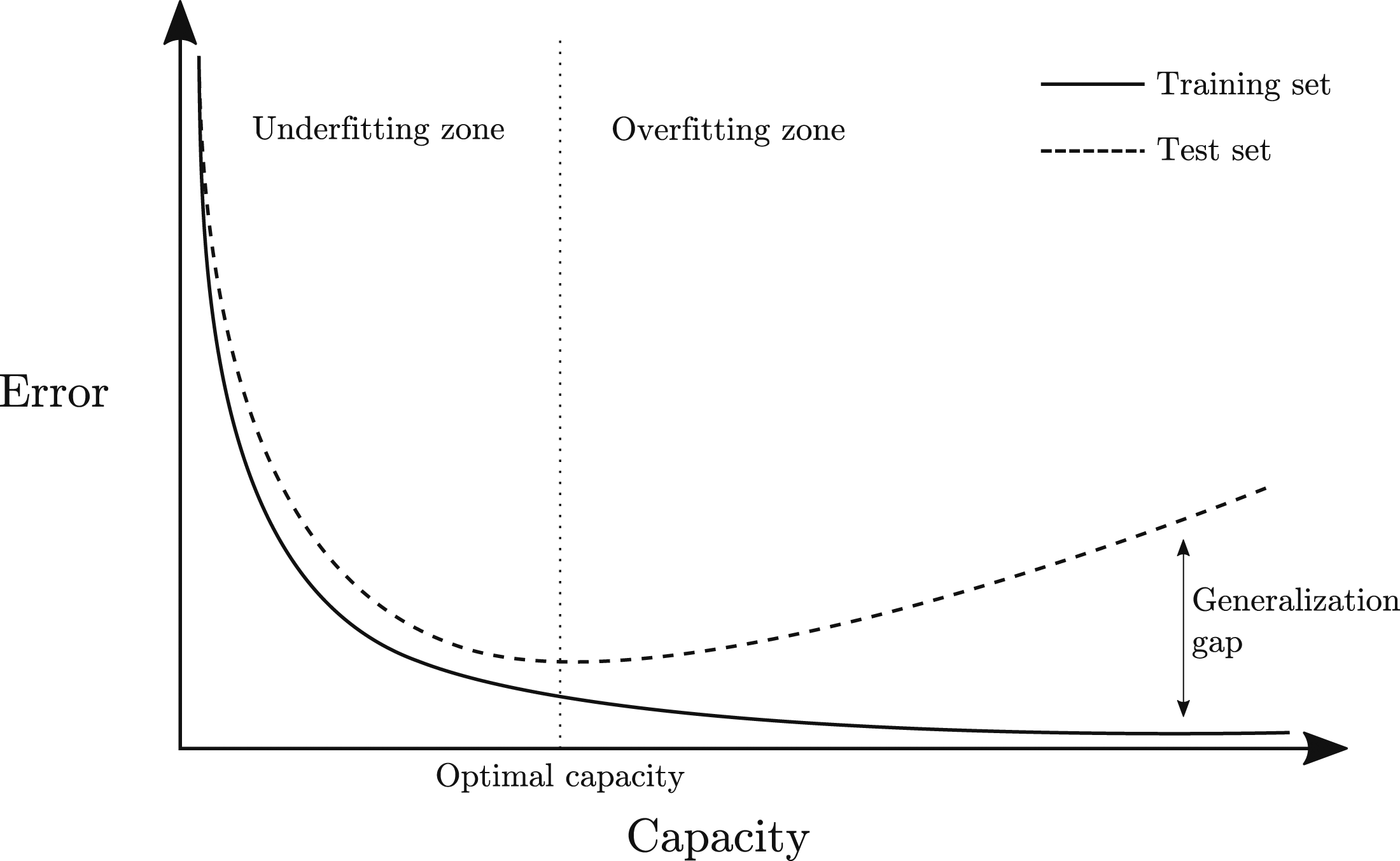

Enhancing the model’s capacity can be achieved in several different ways. One way is by restricting the set of functions an algorithm can choose as its solution through selection of its hypothesis space. In the context of the previous example, this would be allowing higher order polynomials rather than just linear functions for the quadratic and fifth order predictors. Once a family of representative functions has been chosen, there is the issue of finding the optimum function within this, termed the representational capacity of the model. In many cases, finding the optimum function proves to be a difficult optimisation problem.

Recent advancements in improving generalisability suggest that, amongst competing hypotheses that explain the data equally well, the ‘simplest’ should be chosen (Blumer et al., 1989; Goodfellow et al., 2016; Vapnik & Chervonenkis, 1971; Vapnik, 2006, 2013). From the ‘no free lunch’ theorem (Wolpert, 1996), it is impossible to discover the overall optimum ML algorithm but that instead, ML algorithms should be designed to perform well on a specific task by building preferences into the learning algorithm (Goodfellow et al., 2016). Previously mentioned methods of modifying the model’s representational capacity have focused on controlling the hypothesis space of possible solutions; however, there are other ways of controlling a preference for certain solutions, known generally as regularisation. Regularisation is ‘any modification we make to a learning algorithm that is intended to reduce its generalisation error but not its training error’ (Goodfellow et al., 2016). In other words, the chosen learning algorithm can be forced to express a preference for certain solutions in the hypothesis space. Alternative approaches to regularisation which make use of data transformation procedures are particularly useful if the data is well understood. These approaches transform the data to a space where it is well-defined and then train on this new transformed distribution (Notley et al., 2021).

Integrating deep learning approaches (which are data intensive) and scientific theory is considered to be a crucial step to improve model predictive performance whilst respecting natural laws (Reichstein et al., 2019). A promising avenue of research involves guiding the learning of a ML model though introducing a physical consistency penalty as a regularisation procedure (Daw et al., 2020; Jia et al., 2019; Karpatne et al., 2017; Stewart & Ermon, 2017). This framework aims to combine the use of scientific theory and leveraging the power of data-intensive approaches to develop a hybrid approach (as shown in Figure 2) that improves generalisability by guiding the learning process to bias physically valid solutions. Physics-based approaches such as these have been used effectively in a variety of domains such as the geo-sciences community (Karpatne et al., 2017; Muralidhar et al., 2018), power-flow research (Hu et al., 2020) and seismic response modelling (Zhang et al., 2020).

Figure 2.

Schematic representation of physics-guided neural networks in the context of other knowledge discovery approaches. Adapted from Karpatne et al. (2017).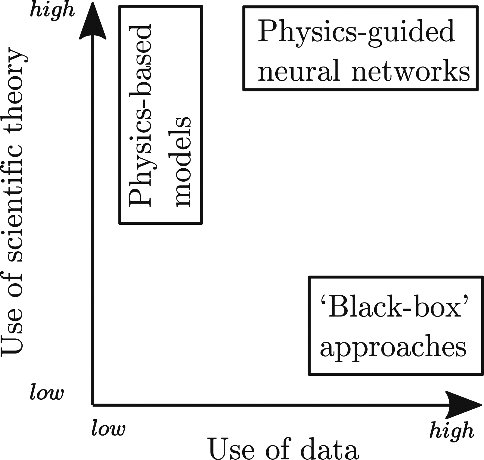

This paper presents a novel use case of this framework in modelling peak specific impulse distributions of near-field blast loading distributions with a comparison against a standard neural network. Firstly, generation of the dataset is discussed. Next, the neural network architecture is developed through a sensitivity study of the network parameters, which is followed by the implementation of a physics-based regularisation. Then the generalisation ability of two neural network architectures (PGNN vs NN) is evaluated by stress-testing the models through withholding specific fractions of the variable distribution. A discussion and concluding remarks are then provided where results show that of the seven stress tests performed, four of the five statistically significant performance premiums were shown by the PGNN. These results indicate that physics-based regularisation procedures should be implemented when specialist knowledge of the problem domain is available.

Surrogate modelling and reduced order models

Data-driven modelling

A surrogate model is an engineering method when an output of interest cannot be directly measured with relative ease. Particularly in engineering, most practical problems require extensive experimental or numerical data to evaluate design decisions. For instance, in aerospace engineering the design of an optimal aerofoil shape for an aircraft wing requires knowledge of airflow parameters for a variety of variables (length, material, angle, etc.), typically determined through simulation (Mack et al., 2007). However, due to the computational expense of running an accurate numerical simulation, obtaining complete information for the design space would carry a considerable time cost and be unsuitable in practice, so a surrogate model is constructed that can evaluate points in the design space that may not necessarily have been explicitly sampled. Surrogate models are constructed using a data-driven, bottom-up approach whereby data sampled from particular simulations or experiments is used to inform a surrogate model (also known as a metamodel or response surface model). The surrogate model then essentially becomes a tool to interpolate in the input–output space of the different design variables.

The data-driven, bottom-up nature of building a surrogate model therefore requires large amounts of data. However, a particular issue in blast engineering is that experimental data can be prohibitively expensive or difficult to obtain due to the high loading magnitudes and sub-millisecond durations of blast events, as mentioned previously. Computational fluid dynamics software provides engineers with the ability to generate the data required to inform an input–output space by solving the physical equations governing fluid flow through discretisation in space and time, and can be validated against known experimental data. The CFD models provide a response for a given set of input parameters, and these are used to fill a parameter space, requiring next the choice of surrogate model to interpolate within this parameter space. A detailed discussion on different types of surrogate model is given in Jin (2005). One such surrogate model is an artificial neural network (ANN) and has been used extensively for this purpose in a variety of disciplines (Ahmadi, 2015; Kim et al., 2015; Papadopoulos et al., 2018; White et al., 2019) and in specific blast engineering applications (Dennis et al., 2020; Flood et al., 2009; Remennikov & Mendis, 2006; Remennikov & Rose, 2007).

ANNs as a surrogate model

Artificial neural networks (ANNs) are collections of connected nodes (also called neurons), inspired by a simplification of neurons in a brain (as per the example shown in Figure 3). They have been used extensively in a wide variety of disciplines due to their ability to act as universal approximators for complex functions. A linear model, which would map inputs to outputs through matrix multiplication, can only represent linear functions, or summations thereof. The universal approximation theorem (Cybenko, 1989; Hornik et al., 1989) states that any feed-forward network with a linear output layer and at least one hidden layer with any ‘squashing’ activation function can approximate any Borel measurable function from one finite-dimensional space to another with any desired non-zero amount of error, provided the network is given enough hidden units (Goodfellow et al., 2016). Similarly, an ANN can approximate any function mapping from any finite dimensional discrete space to another. This ability to approximate non-linear functions makes ANNs a suitable choice for a wide variety of procedures, and particularly for recreating the non-linear physical phenomena seen in near-field explosive events.

Figure 3.

Example neural network architecture with two input nodes, three nodes in a hidden layer and one output node.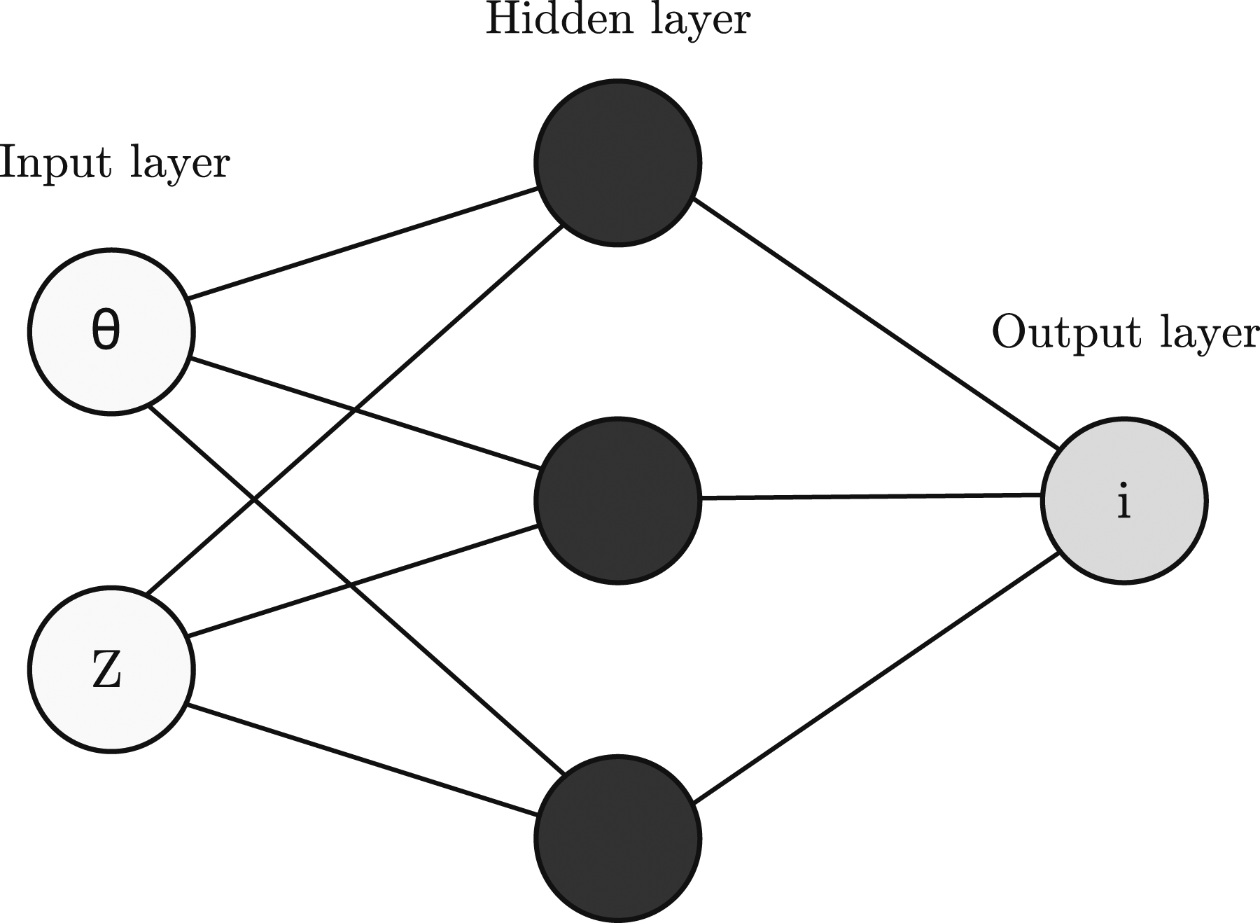

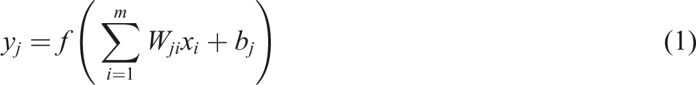
The hidden layers in an ANN consist of interconnected neurons. Information is conveyed through these neurons with a series of weights and biases, transmitted with non-linear activation functions. To train an ANN, the optimal values for weights and biases must be found, which typically involves two stages: ‘feedforward propagation’ and ‘error backpropagation’. Considering equation (1)

y_{j} = f (\sum_{i = 1}^{m} W_{j i} x_{i} + b_{j})

(1)

where y_j is the output for the jth neuron in the current hidden layer, the output of each neuron is obtained by inputting into activation function, f, the product of the weight connecting the two neurons, W_ji the input, x_i and then adding a bias term, b_j. This summation is continued for all hidden units until reaching the output layer, finalising the feedforward propagation. The prediction from the network can be compared to a target output and an error can be calculated (such as mean squared error). Once the error has been calculated, the learning algorithm can adjust the weights and biases after a set number of trials (the batch size) to minimise the error between model predictions and target values. This is termed ‘error backpropagation’ and is repeated for a given number of complete passes through a dataset (the epoch number).

As shown previously in Figure 1, as the capacity of an ML model increases, as does the chance of overfitting. Specific to an ANN, there are several variables that can be changed in order to find the ‘optimal capacity’. Firstly, considering the structure of the network itself, the capacity of the model can be altered by increasing the number of layers, the nature of these layers, number of neurons in each layer and the connectivity of these neurons. If every neuron in each layer is connected to every other neuron in adjacent layers, this is known as ‘fully connected’ or ‘dense’. This is the structure of traditional multi-layer perceptrons. An alternative class of neural networks are convolutional neural networks (CNNs), which also consist of input layers, hidden layers, and output layers, but the hidden layers perform convolutions on input data. CNNs have been shown to be useful in many image analysis tasks (Albawi et al., 2017), with some applications in blast analysis (Xu et al., 2021). Finding the optimal structural configuration of an artificial/convolutional neural network is a challenging task and has been shown to be case-dependent and largely data-driven in nature (Dsouza et al., 2020).

A central problem in ML is improving the ability of a model to generalise to unseen data. One such approach that focuses on reducing the test error (typically at the cost of an increased training error) is regularisation, as mentioned previously. There are several approaches to regularisation; some target the parameters of the model by restricting or constraining their values in some way or including additional penalties, thereby encoding some prior knowledge into the model. One common example of a regularisation procedure is ‘weight decay’, where a sum is minimised that involves an additional criterion that adds a preference for model parameter weights to have a smaller L² norm, as shown in equation (2) (Goodfellow et al., 2016)

J (w) = M S E_{t r a i n} + λ w^{T} w

(2)

where J(w) is the cost function to minimise, MSE_train is the mean squared error of training data, w is the parameter weights and λ is a hyper-parameter. This is an obtrusive form of regularisation as the objective function of the minimisation procedure is directly modified. Because of this, the choice of the hyper-parameter λ is crucial: too small and the model will overfit to the data, whilst too large and it will underfit. Another common regularisation procedure is known as ‘early-stopping’, and is simple to implement and highly effective. This approach can be considered an algorithm for selecting the optimum model parameters, as throughout training the model weights and biases are being changed. By implementing early stopping, the model parameters that show the best generalisability are returned.

Further regularisation techniques rely on combining several different trained models, in the hope that their average, aggregate performance shows better generalisability, known as bagging (Breiman, 1996). This general strategy is known as model averaging and similar methods are known as ensemble methods. Neural networks often benefit from model averaging of some kind due to the differences in parameter initialisation or other hyper-parameters (Goodfellow et al., 2016). On a similar theme, another particularly useful form of regularising ANNs is known as ‘dropout’ (Srivastava et al., 2014). When a fully connected layer has a large number of neurons, there is likely to be some co-adaption. Co-adaption refers to the scenario where multiple neurons extract the same information or features from a set of input data, the detriment of this is an inefficient use of computational resources and an increased risk of overfitting by adding more significance to certain model features. In dropout, the ensemble of all the model subnetworks that can be formed by removing units from a base network are trained. For an extensive overview of further regularisation procedures, see Goodfellow et al. (2016).

Dataset overview

The dataset was generated from CFD simulations using APOLLO Blastsimulator, an explicit CFD software which solves the conservation equations for transient flows of compressible fluid mixtures (inviscid and/or non-heat conducting, inert and/or chemically reacting). APOLLO uses a HLL-type Reimann solver, particularly suited for problems involving rapid changes in pressure and density, and high speed flows, and is second order accurate owing to the tri-linear reconstruction of cell-centred conservative variables (Fraunhofer EMI, 2018).

Analyses were performed in quarter symmetry. In order to prevent spurious expansion waves from the edge of the domain corrupting the results (Rigby et al., 2014b), the domain side lengths were set to the minimum of either 1.5 m or 1.3 times the distance from the centre of the target to the most remote gauge (Pannell et al., 2021). The mesh size was set at 100 mm zone length and resolution level 5 (minimum element size of 100/2⁵ = 3.125 mm).

The dataset consists of peak specific impulse distributions from 100 g spheres of PE4 located between 0.05 m and 0.26 m normal distance from the centre of the charge to the surface of the target, termed ‘stand-off’ distance. This is equivalent to a scaled distance range of 0.11–0.55 m/kg^1/3 according to cube-root or Hopkinson–Cranz scaling (Cranz, 1926; Hopkinson, 1915), where scaled distance, Z, is given by S/W^1/3, where S is stand-off distance and W is the mass of explosive. The explosives were modelled using Apollo’s in-built model for C4 explosive, with Klomfass Afterburning Model and Chapman–Jouguet detonation model both used.

For each analysis, 150 gauges are linearly spaced along the target surface at angles of incidence between 0 and 60°, where angle of incidence is defined as the angle between the outward normal of the surface and the direct vector from the explosive charge to that point (Rigby et al., 2015b). Each gauge outputs pressure-time histories at that location, which are numerically integrated (with respect to time) in postprocessing to yield specific impulse-time histories. The maximum of each of these is taken to provide the distribution of peak specific impulse.

In summary, there are 18 CFD experiments with 150 values of peak specific impulse for each, resulting in a dataset of 2700 data points. An overview of this dataset is given in Figure 4b, with a schematic detailing the generation of this dataset shown in 5a. Mesh sensitivity and experimental validation for APOLLO has previously been conducted in Pannell et al. (2021). Here, numerical results were compared to experimental data of Rigby et al. (2019a), measured using the Characterisation of blast loading apparatus (Clarke et al., 2015). The apparatus consists of arrays of Hopkinson (1914) pressure bars mounted flush with the surface of a nominally rigid target plate, and provides spatial and temporal distributions of loading, that is, pressure-time and impulse-time histories, and peak pressure and peak specific impulse distributions. In this validation exercise, the loading from 100 g PE4 spheres at 80 mm perpendicular stand-off distance (to the charge centre) was measured out to 100 mm from the centre of the target plate. An example of the validation of APOLLO is given in Figure 5.

Figure 4.

(a) Experimental schematic for the dataset generation: S is perpendicular stand-off distance between spherical charge and reflecting surface, gauges were placed along the perpendicular length r. (b) computational fluid dynamics dataset: filled contours of scaled peak specific impulse for full dataset, 0.11–0.55 m/kg^1/3.

Figure 5.

Validation of Apollo using experimental data (Rigby et al., 2019a) from 100 g PE4 sphere at 80 mm (to charge centre) stand-off distance: (a) overpressure history at 25 mm from the plate centre (θ = 17°); (b) peak specific impulse distributions at 0–100 mm distance from the plate centre. Figure adapted from Pannell et al. (2021).

Each input for the NN is shown in Table 1, with an example entry: X represents the input vectors and Y represents the labelled output so that in its entirety the dataset is a (2700, 3) array. The variables X₁ and X₂ are minmax scaled across the entire dataset with a feature range of [0, 1]. The output, Y, has a log-normal distribution and was scaled via a power transform; a family of parametric, monotonic transformations applied to provide normality and homoscedasticity to the training data for ease of model training, using the method described in Yeo and Johnson (2000). The result of the power transform is given in Figure 6. The data transformations are completed after any data splitting procedures are undertaken to ensure there is no data leakage from the transformation.

Table 1.

Example dataset information.

X ₁	X ₂	Y
Scaled distance (m/kg^1/3)	Angle of incidence	Peak specific impulse (MPa.ms)
0.1	15	45.87

Figure 6.

Unscaled Y dataset showing a log-normal distribution (left) and the resulting power transformation (right).

Training and network architecture

To create and train the networks, the Keras package with tensorflow backend (Chollet et al., 2015) was used. The Adadelta (Zeiler, 2012) gradient descent algorithm was chosen which has the added benefit of not requiring a default learning rate. 10 000 epochs with early stopping set at 500 epochs was implemented to prevent over-fitting, with a batch size of 32. Activation functions for the hidden units were set as hyperbolic tangent, and layer weights initialised with the Glorot normal initialiser (Glorot & Bengio, 2010). K-fold cross-validation was implemented with five splits, following an initial data split of 25% data randomly removed, this data splitting schematic is summarised in Figure 7. The networks to be examined all had one hidden layer, and are fully connected.

Figure 7.

Example schematic of splitting the dataset prior to and during training and the subsequent k-fold cross-validation. The initial 25% of test data removed is never seen by the model during training.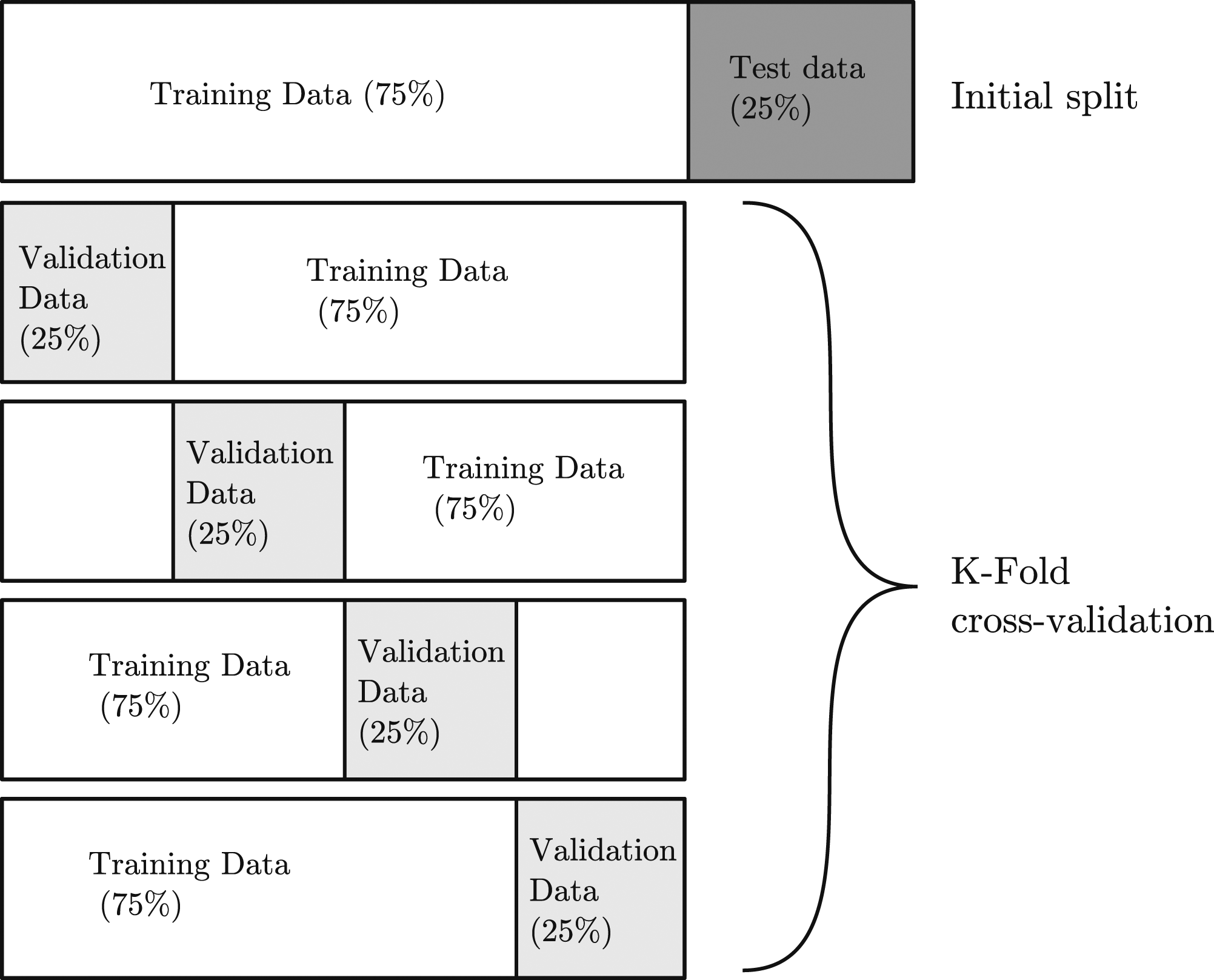

Initially, a varying number of hidden units were examined, from 1 to 8. The results of these analyses are presented in Figure 8. Ideally, the structural optimisation of the network would be performed in parallel to the parametric optimisation via an overarching, many-objective process (Jin & Sendhoff, 2009; Loghmanian et al., 2012), though this is considered to be beyond the scope of this paper. Three separate sub-figures provide different metrics: mean squared error (Figure 8(a)), mean absolute error (Figure 8(b)) and coefficient of determination (Figure 8(c)). For all analyses, the metrics are assessed for the three separate data portions: test, train and validation as previously summarised in Figure 7. If large discrepancies occur between the different data types, this can be indicative of over-fitting issues, as the models may perform far better on ‘seen’ data rather than ‘unseen’ data. As shown, there is a general trend of error reducing as the number of neurons increases, though this plateaus after four neurons, suggesting that four neurons provide sufficient predictive capability. Furthermore, from two neurons and upwards, there are no significant discrepancies between the different data types, suggesting that the model is not over-fitting. For later analyses, a network with four hidden units was chosen to take forward.

Figure 8.

Hyper-parameter configuration with various performance metrics shown on the unseen test data. Error bars are standard deviation: (a) Mean squared error of model predictions for varying number of neurons in hidden layer (b) Mean absolute error of model predictions for varying number of neurons in hidden layer (c) Coefficient of determination of model predictions for varying number of neurons in hidden layer.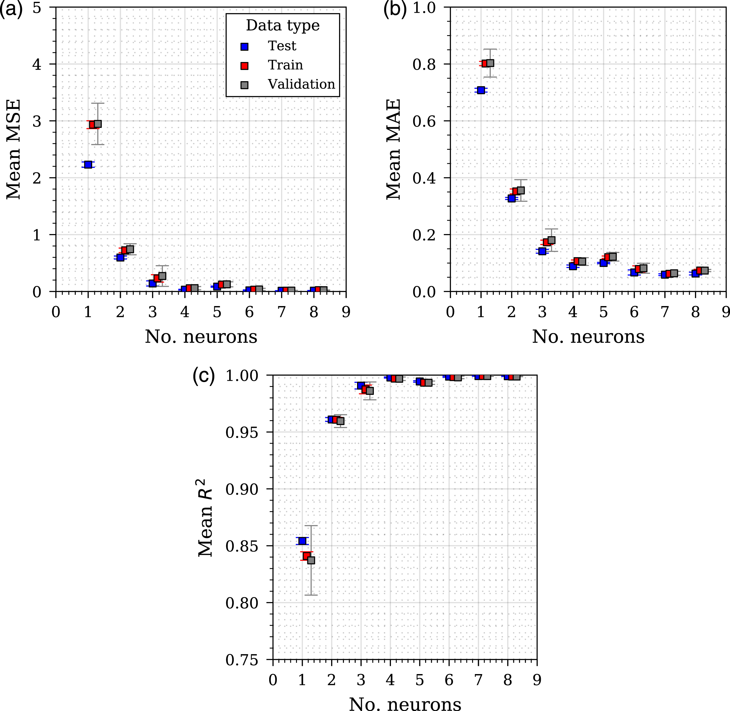

With the network architecture chosen, it is useful to gain an insight into the model learning performance of this network to check further for over-fitting and to confirm that the model is learning as expected. Training histories from the cross-validation are provided in Figure 9, which shows the loss from validation and training data during training. As demonstrated, the performance consistently improves as the number of epochs increases, and also improves for each fold of the cross-validation, suggesting that the network is learning effectively. The generalisation gap between the training and validation set is small and remains fairly constant throughout which is demonstrative of a good fit. On initial inspection there appears to be some stochastic behaviour in the later folds, however considering the magnitude of the losses here these are not considered to be a cause for concern and it can be concluded that the model shows a good fit.

Figure 9.

Training loss histories for each of the 5-fold cross-validation. Analyses represent the chosen network with four hidden units: (a) First fold (b) Second fold (c) Third fold (d) Fourth fold (e) Fifth fold.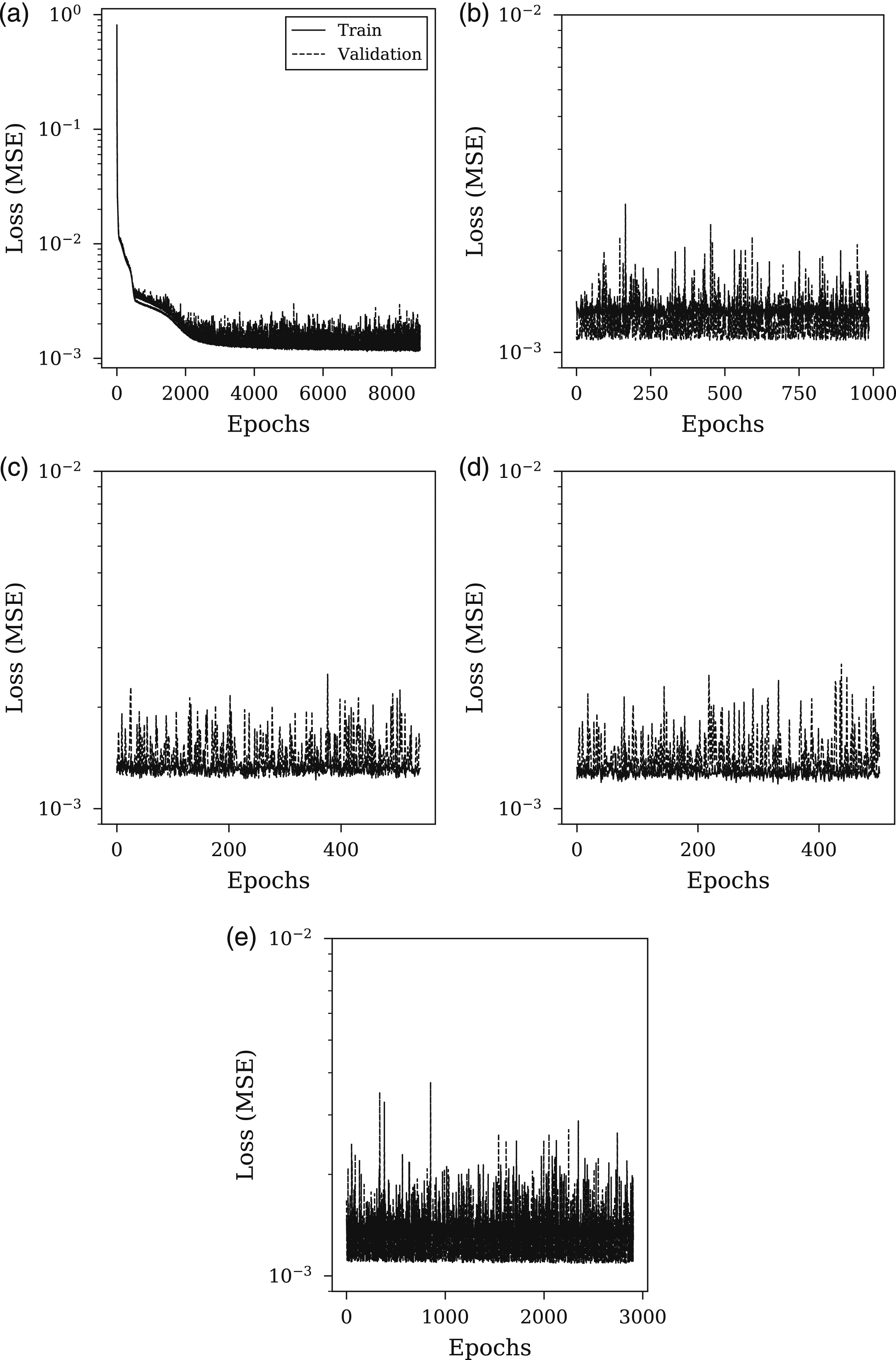

A physics-based regularisation procedure

All regularisation methods are attempting to improve the generalisability of a ML model. That is, how it performs on unseen data. Regularisation would not be required if the optimum structure, learning algorithm, and data transformation for a given NN were known a priori. Typical approaches for training models without physical constraints involve minimising empirical loss (mean square error, MSE) of model predictions 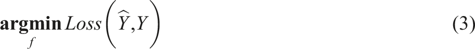$(\hat{Y})$ on the training data (Y) whilst maintaining low model complexity as follows in equation (3)

\underset{f}{argmin} L o s s (\hat{Y}, Y)

(3)

where Y refers to target values. Through an additional physical inconsistency term, the model will now punish predictions that are not valid with respect to the physical law that is incorporated. This is demonstrated in equation (4) (Karpatne et al., 2017) with the addition of a physical loss function,

L o s s . P h y (\hat{Y})

, and the corresponding hyper-parameter (λ_Phy)

\underset{f}{argmin} L o s s (\hat{Y}, Y) + λ_{P h y} L o s s . P h y (\hat{Y})

(4)

In this research, we present an implementation of a physics-based regularisation procedure based on each of the input features. Firstly, we make use of prior knowledge that peak specific impulse decays monotonically with scaled distance for a given angle of incidence (Pannell et al., 2021), which allows the implementation of a monotonic loss constraint. This monotonic loss constraint is in place to only penalise values that do not satisfy the requirement, implemented through the use of a rectified linear unit activation function (ReLU). The ReLU function is represented mathematically as f(x) = max(0, x). Then the physical loss function returns the following, adapted from Karpatne et al. (2017)

L o s s . P h y_{1} (\hat{Y}) = \frac{1}{n} \sum_{i = 1}^{n - 1} ReLU (f (X_{1, i + 1}, X_{2}) - f (X_{1, i}, X_{2}))

(5)

where X₁ refers to scaled distance and hence X_1,0 being the smallest value in the dataset with f(X_1,i, X₂) representing the model prediction for a given angle of incidence, X₂. The subscript i indicates the index of the vector X₁. It is important to remember here that the minimum X₁ value (X_1,0) will result in the maximum output (Y), as increasing the scaled distance between charge and target will increase X₁ and decrease Y. Therefore if the model predicts a greater output at a larger scaled distance (X_1,i+1) than it does for a smaller scaled distance (X_1,i), this result is non-physical and is punished by the monotonic loss constraint.

Similarly, prior knowledge (Pannell et al., 2021) that peak specific impulse decays monotonically with angle of incidence for a given scaled distance (where scaled distance is calculated from the hypotenuse distance between the charge centre and the measurement location) allows the implementation of a second monotonic loss constraint

L o s s . P h y_{2} (\hat{Y}) = \frac{1}{n} \sum_{i = 1}^{n - 1} ReLU (f (X_{1}, X_{2, j + 1}) - f (X_{1}, X_{2, j}))

(6)

where for a given X₁, the maximum output will be obtained at X_2,0, decaying monotonically as X₂ increases. Therefore, if the model predicts a greater output at a larger angle of incidence (X_2,j+1) than it does for a smaller angle of incidence (X_2,j), this result is also deemed non-physical and is again punished by the model. Combining the two additional physical loss constraints (equations (5) and (6)) into equation (3), we obtain the final model loss function

\underset{f}{argmin} L o s s (\hat{Y}, Y) + λ_{P h y, 1} L o s s . P h y_{1} (\hat{Y}) + λ_{P h y, 2} L o s s . P h y_{2} (\hat{Y})

(7)

where

λ_{P h y, 1} L o s s . P h y_{1} (\hat{Y})

refers to the monotonic loss constraint with respect to scaled distance and

λ_{P h y, 2} L o s s . P h y_{2} (\hat{Y})

refers the monotonic loss constraint with respect to angle of incidence.

Implementation of the physical loss function requires values for the hyper-parameters to be found. A sensitivity study was conducted and with the performance metric set as root mean square error (RMSE) on unseen, test data. The sensitivity study for these hyper-parameters (λ_Phy,1 and λ_Phy,2) assessed six logarithmically spaced values varying between 10⁰ and 10⁵. The results from this sensitivity study are given in Figure 10, with λ_Phy,2 shown on the x-axis and λ_Phy,1 on the y-axis, with the colour presenting the mean value for test RMSE (from the five folds of the cross-validation). The global optimum hyper-parameter values from this exercise were seen to be λ_Phy,1 = 10⁵ and λ_Phy,2 = 10². The values taken forward however were λ_Phy,1 = 10⁴ and λ_Phy,2 = 10⁴; although not the global optimum for each, these values were in the top 20% of recorded RMSE values and were the top hyper-parameter set under the constraint λ_Phy,1 = λ_Phy,2. This constraint was considered to be suitable to provide no bias towards the features X₁ or X₂, and on inspection the training history for this hyper-parameter set demonstrated the penalty was working effectively and therefore was a suitable choice to take forward.

Figure 10.

Grid search of λ_Phy,1 and λ_Phy,2.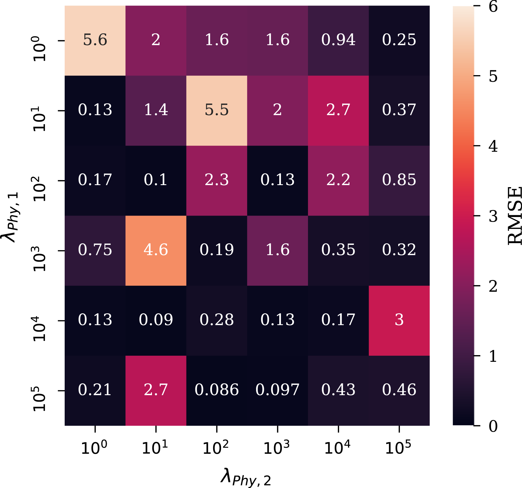

Stress-testing evaluation

Overview of stress-testing procedure

It is useful for predictive models in blast loading to be able to generalise both beyond the limits of the dataset and between points within the dataset. A model which is able to generalise in this way would be particularly beneficial to bypass practical/physical constraints relating to availability of equipment, placement of gauges and limitations of the recording equipment. For example, there may be practical limitations which prevent tests from being performed at certain scaled distances (limitations on robustness and survivability of recording equipment at smaller scaled distances, excessive signal to noise ratios at larger scaled distances) as well as potential issues relating to limited availability of diagnostics which may result in a sparse dataset. Understanding how accurately a model can extrapolate and interpolate has significant implications for the design of future experiments: such knowledge will provide experimentalists with a clear steer on typical areas of high sensitivity and therefore those with significant contributions to the overall accuracy of ML approaches, as well as areas where detailed measurements may not be required.

The stress-testing evaluation procedure therefore aims to investigate two themes of estimation ability: interpolation and extrapolation, as well as their dependencies on the availability of data to make accurate predictions. Herein, the dataset comprises three variables: X₁ (Z, scaled distance), X₂ (θ, angle of incidence) and Y (peak specific impulse). By restricting the availability of certain regions of each variable distribution, the ability of the model to generalise can be assessed for each given variable. Seven types of stress-test were performed, assessing either extrapolation or interpolation ability with 25% of the dataset removed. For each stress-test, each network was trained to 100 epochs, and this procedure repeated 25 times. Early stopping was used in all cases with a patience value set to 5 epochs. The information for each type of stress-test is summarised below:

1. Interpolation

(a) Mean X₁ values removed

(b) Mean X₂ values removed

2. Extrapolation

(a) Maximum X₁ values removed

(b) Minimum X₁ values removed

(d) Minimum X₂ values removed

The architecture of the neural networks (NN and PGNN) follows that summarised previously, with the two additional hyper-parameters λ_Phy,1 = 10⁴ and λ_Phy,2 = 10⁴ included for the PGNN. Before the training process, various proportions of the data were removed, dependent on the mode of stress-testing, and the model performance was evaluated in each case by recording the RMSE on the removed, unseen test data. By also analysing the training history in each simulation, a physical inconsistency term can be quantified as the proportion of total epochs where physically invalid predictions are made (Karpatne et al., 2017), this will provide an insight into how ‘physically valid’ each network is. For clarity, if physically inconsistent predictions are made in 4 of the 100 epochs, then the physical inconsistency measure will be 0.04, where a physically inconsistent prediction is defined as a positive result from equations (5) or (6).

Results

Interpolation

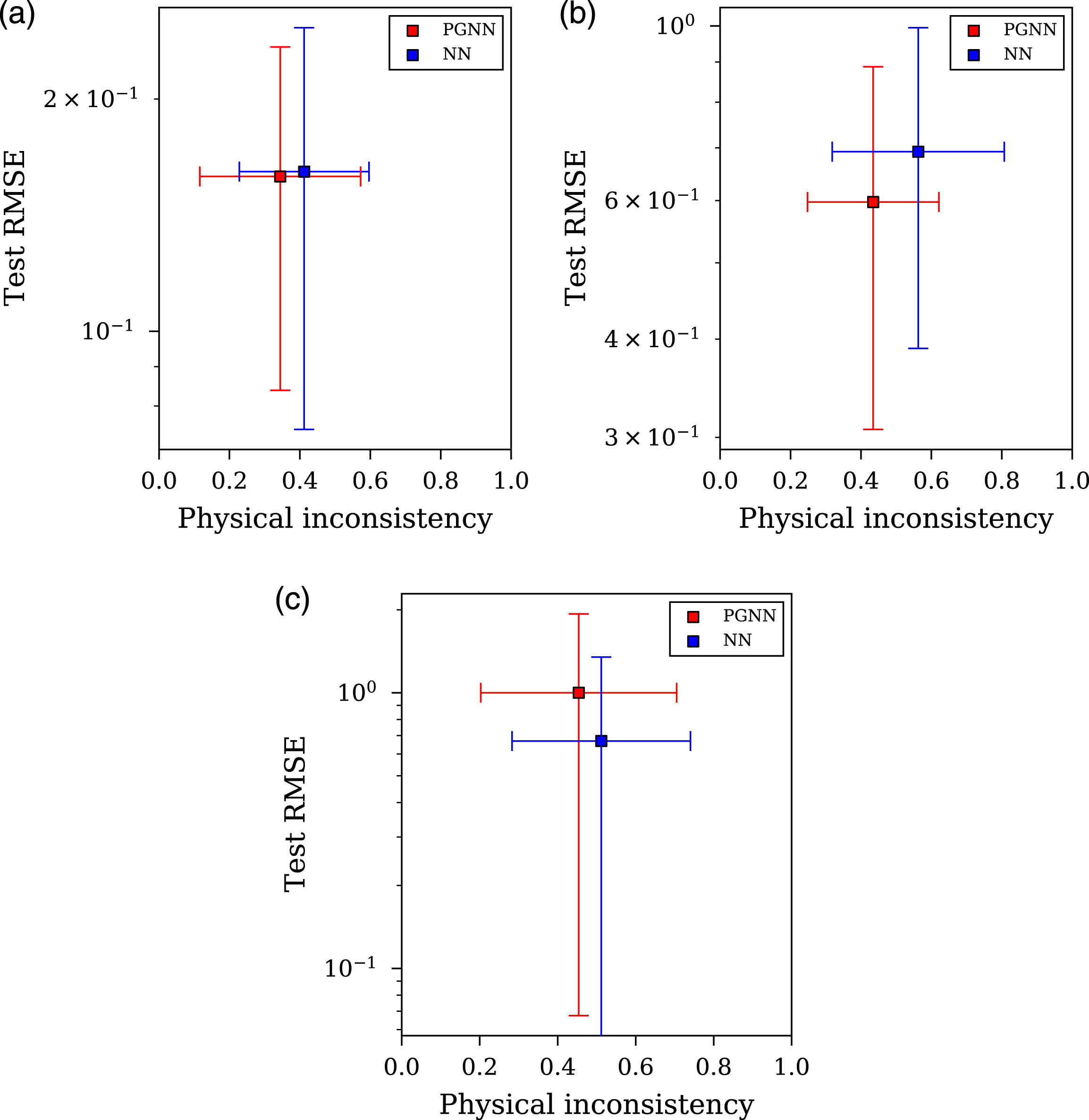
The first theme of stress-testing aims to assess the estimation ability of the models to interpolate between the upper and lower limits of the dataset. Firstly, removing the region of the variable distribution around the mean of scaled distance (X₁), and angle of incidence (X₂), and finally removing data randomly across the distribution space. For each analysis, the distribution of the dataset with 25% of the variable removed is presented in Figure 11, with the RMSE on unseen test data and physical inconsistency values presented in Figure 12. Due to the cross-validation procedure and the simulation repeats, more than one value for RMSE, and physical inconsistency, is provided for each NN architecture; therefore, the standard deviation of these values are plotted as error bars whilst the mean indicated as the scatter point for each architecture. Also shown in Figure 11 are a representation of the data remaining for the training process after removal according to the stress test. Here, a black pixel denotes the presence of labelled data for that combination of X1 and X2, whereas a white pixel denotes the absence of data.

Figure 11.

Interpolation stress tests, effects of data removal on the data distributions. Distribution of Y (peak specific impulse) before and after data removal (left); distribution of X₁ (scaled distance) and X₂ (angle of incidence) after data removal (right): (a) Removing 25% of data around the mean X₁ value (b) Removing 25% of data around the mean X₂ value (c) Removing the 25% of X values randomly.

Figure 12.

Results showing root mean square error of removed test data and physical inconsistency for various interpolation stress-test procedures: (a) Removing 25% of data around the mean of X₁ (scaled distance) (b) Removing 25% of data around the mean of X₂ (angle of incidence) data (c) Removing the 25% of X data randomly.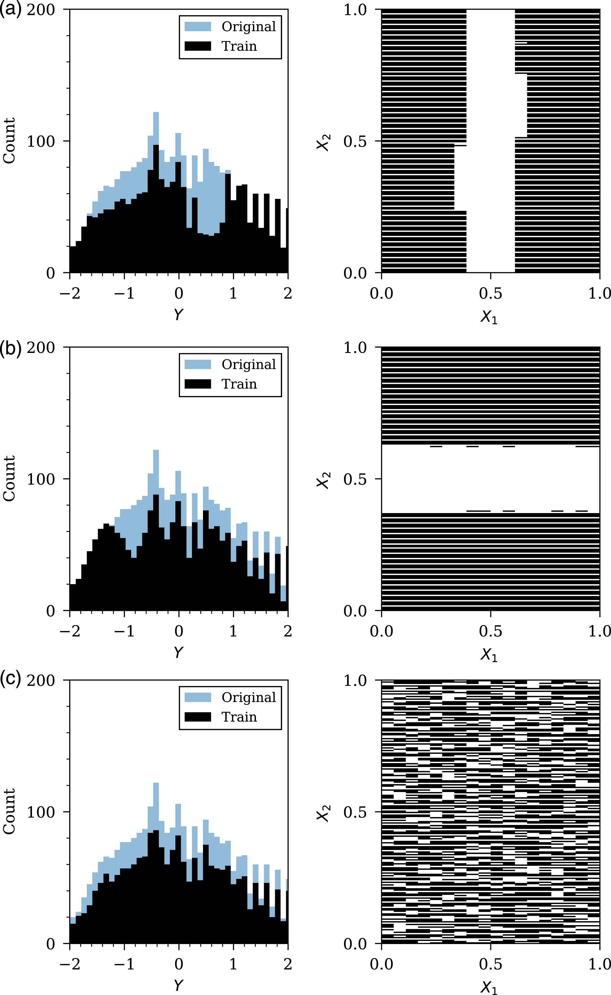

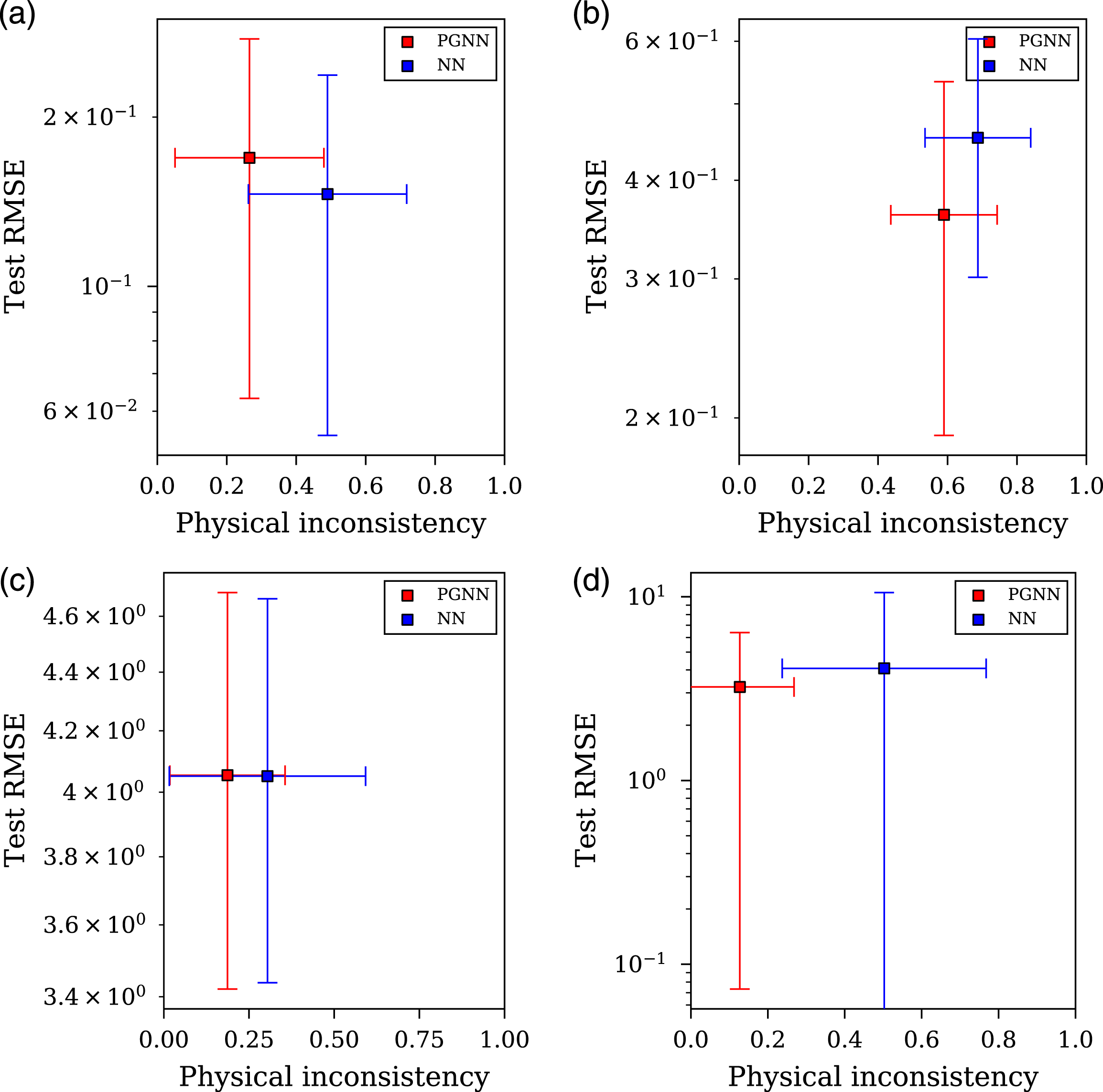
Extrapolation

The second theme of stress-testing aims to assess the estimation ability of the models to extrapolate beyond the upper and lower limits of the dataset. Firstly, removing the maximum values of scaled distance (X₁) and maximum values of angle of incidence (X₂). It is important to note here that the minimum values of peak specific impulse correspond to the maximum values in scaled distance and angle of incidence (due to the monotonic decrease of specific impulse with an increase in these variables). For each analysis, the distribution of the dataset with 25% of the variable removal is presented in Figure 13, with the RMSE on unseen test data and physical inconsistency values presented in Figure 14. As mentioned previously, due to the cross-validation procedure and the simulation repeats, more than one value for RMSE, and physical inconsistency, is provided for each neural network architecture. The standard deviation of these values are plotted as error bars whilst the mean is given by the scatter point for each architecture.

Figure 13.

Extrapolation stress tests, effects of data removal on the data distributions. Distribution of Y (peak specific impulse) before and after data removal (left); distribution of X₁ (scaled distance) and X₂ (angle of incidence) after data removal (right): (a) Removing the maximum 25% of X₁ values (b) Removing the maximum 25% of X₂ values (c) Removing the minimum 25% of X₁ values (d) Removing the minimum 25% of X₂ values.

Figure 14.

Results showing root mean square error of removed test data and physical inconsistency for various extrapolation stress-test procedures: (a) Removing the maximum 25% of X₂ (scaled dis- tance) data (b) Removing the maximum 25% of X₂ (angle of incidence) data (c) Removing the minimum 25% of X₂ (scaled dis- tance) data (d) Removing the minimum 25% of X₂ (angle of incidence) data.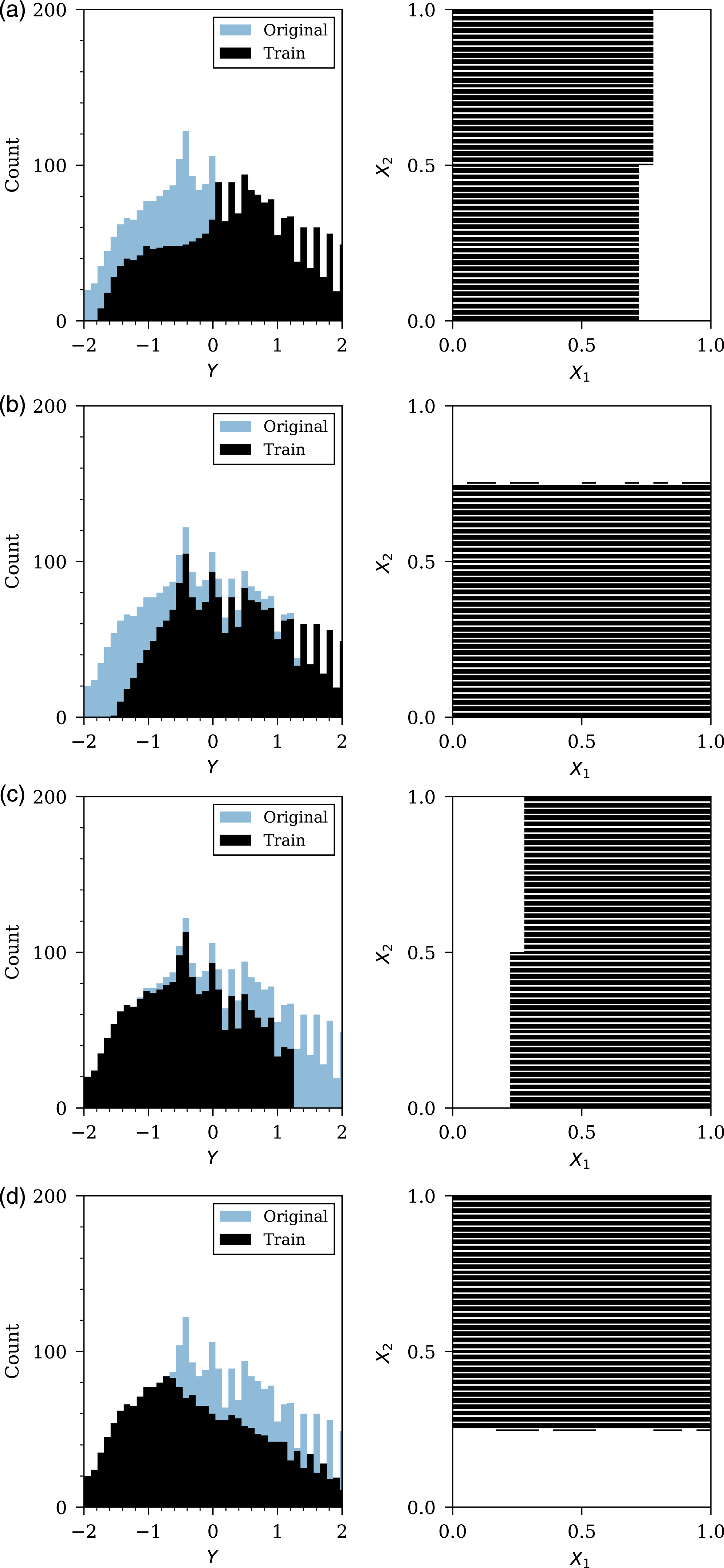

Discussion

The results from the stress-testing evaluation for the NN and PGNN are compared in Table 2. In order to check the statistical significance of the results from each stress-test, two-tailed Kolmogorov–Smirnov tests (Hodges, 1958) have been performed in each case. This is a two-tailed test for the null hypothesis that two independent samples are drawn from the same continuous distribution. In the perspective of these analyses, the test checks whether the RMSE or physical inconsistency values recorded by each model are drawn from the same distribution, therefore suggesting no statistically significant difference.

Table 2.

Mean results from each stress-testing evaluation of NN and PGNN models. Entries in bold indicate a statistically significant difference (p < 0.10) from the Kolmogorov–Smirnov two-tailed test statistic (Hodges, 1958) for both performance premium and physical inconsistency (two-tailed p-value).

Stress-test		Test RMSE		Physical inconsistency
		NN	PGNN	NN	PGNN
Extrapolate	Maximum X₁	0.15	0.17	0.49	0.27
	Maximum X₂	0.45	0.36	0.69	0.59
	Minimum X₁	4.05	4.05	0.30	0.19
	Minimum X₂	4.08	3.23	0.50	0.19
Interpolate	Mean X₁	0.16	0.16	0.41	0.34
	Mean X₂	0.69	0.60	0.56	0.43
	Random	0.67	1.00	0.51	0.45

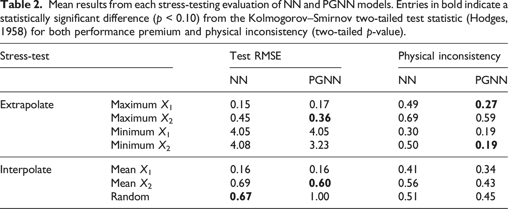
It is clear that the PGNN outperforms the NN when extrapolating and interpolating with respect to X₂, whilst extrapolation and interpolation with respect to X₁ appears insensitive to network type. This could suggest that the hyper-parameter λ_Phy,1 is not set at an optimum level and could be adapted to further improve the method presented in this paper. There were three statistically significant findings with respect to test RMSE values: the results show that the PGNN significantly outperformed the NN when extrapolating beyond the maximum of X₂, and removing data around the mean of X₂, whereas the NN outperformed the PGNN when data was removed randomly.

The PGNN showed a statistically significant performance premium when extrapolating beyond the maximum of X₁, and beyond the minimum of X₂ with respect to physical inconsistency. When considering performance with respect to physical inconsistency on aggregate, however, it is shown that the PGNN outperforms the NN across all seven stress tests (even those not deemed statistically significant). If the null hypothesis of equal mean performance between the PGNN and NN with respect to physical inconsistency is considered, the observed outperformance in all seven modes of testing has a probability of 0.007 (p < 0.05); a clear performance premium.

These results are highly promising from an engineering perspective. The PGNN model is constructed so that it is far less likely than the NN to under-predict when extrapolating. Essentially, the PGNN contains inbuilt conservatism in model predictions. This ensures that when analysing structures subjected to blast loading following close-in detonation of a high explosive, solutions informed by PGNNs are more likely to be conservative; an approach that whilst not maximising efficiency will ensure safety. Extrapolating beyond data limits should always be handled with caution in predictive models, however the PGNN approach explored in this article provides additional conservatism and maintains physical consistency if extrapolation is ever required.

Summary

This paper presents a novel application of a physics-based regularisation framework for neural networks in the application of predicting blast loading following detonation of an explosive charge. The physics-based regularisation is shown to provide statistically significant performance improvements over traditional neural network procedures when generalising beyond the dataset through extrapolation and interpolation with regards to accuracy (shown via test RMSE) and physical validity (via a physical inconsistency metric). This finding provides positive evidence towards using physics-based regularisation when training ML models, and the use of ML models generally, especially in applications involving the prediction of blast loads resulting from the detonation of high explosives.

An initial parameter search study was completed for a traditional neural network (NN), with the chosen parameters also used in the physics-guided neural network (PGNN). Both models were stress-tested through various data holdout approaches, and their ability to predict high explosive blast loading were comprehensively evaluated and compared. It is found that the PGNN out-performed the NN in 57% (4/7) of the stress tests (lower RMSE), and exhibited lower physical inconsistency in the training process in 100% (7/7) of the stress tests (p < 0.05). With respect to the specific mode of stress-testing, of the PGNN’s 11 performance premiums, 4 were found to be statistically significant: RMSE when extrapolating with respect to maximum X₂ and interpolating with respect to mean X₂, and physical inconsistency when extrapolating with respect to maximum X₁ and minimum X₂ (where X₁ is scaled distance and X₂ is angle of incidence).

Additionally, this research has considered the importance of careful consideration of the parameters which govern a network’s ability to generalise, and subsequent implications for experimental design. The results demonstrate the feasibility and enhanced accuracy achievable when developing ML models to predict near-field blast loading. As a continuation of this research, future work will involve incorporating different charge types (Grisaro et al., 2021), shape effects (Rigby et al., 2021) and blast wave clearing (Rigby et al., 2013) as features in the model. Further, incorporating more complex physics (through implementing a non-linear loss constraint instead of the monotonic loss constraint) will enable the possibility of improved PGNN performance through transfer learning. Developments in this area will facilitate more accurate probabilistic-based approaches to engineering design and risk mitigation that encompass a more complex suite of scenarios than is capable presently.

Footnotes

Acknowledgements

The authors acknowledge a Python script from the implementation by that was used as a core template to develop.

Declaration of conflicting interests

The author(s) declared no potential conflicts of interest with respect to the research, authorship, and/or publication of this article.

Funding

The author(s) disclosed receipt of the following financial support for the research, authorship, and/or publication of this article: Jordan J Pannell gratefully acknowledges the financial support from the Engineering and Physical Sciences Research Council (EPSRC) Doctoral Training Partnership.

ORCID iDs

Jordan J Pannell

Sam E Rigby

References

Ahmadi

(2015) ‘Developing a robust surrogate model of chemical flooding based on the artificial neural network for enhanced oil recovery implications’. Mathematical Problems in Engineering.

Albawi

Mohammed

Al-Zawi

(2017) Understanding of a convolutional neural network. In: 2017 international conference on engineering and technology, Antalya, Turkey, 21–23 August 2017. Ieee: ICET, pp. 1–6.

Alterman

Stewart

Netherton

(2019) Probabilistic assessment of airblast variability and fatality risk estimation for explosive blasts in confined building spaces. International Journal of Protective Structures 10(3): 306–329.

Baker

(1973) Explosions in Air. Austin, TX, USA: University of Texas Press.

Blumer

Ehrenfeucht

Haussler

, et al. (1989) Learnability and the vapnik-chervonenkis dimension. Journal of the ACM 36(4): 929–965.

Breiman

(1996) Bagging predictors. Machine Learning 24(2): 123–140.

Campidelli

Tait

El-Dakhakhni

, et al. (2015) Inference of blast wavefront parameter uncertainty for probabilistic risk assessment. Journal of Structural Engineering 141(12): 04015062.

Chollet

(2015) Keras. https://github.com/fchollet/keras

Clarke

Fay

Warren

, et al. (2015) A large scale experimental approach to the measurement of spatially and temporally localised loading from the detonation of shallow-buried explosives. Measurement Science and Technology 26: 015001.

10.

Cloete

Nurick

(2016) Blast characterization using a ballistic pendulum with a centrally mounted Hopkinson bar. International Journal of Protective Structures 7(3): 367–388.

11.

Cranz

(1926) Lehrbuch der Basllistik. Berlin, Germany: Springer.

12.

Cybenko

(1989) Approximation by superpositions of a sigmoidal function. Mathematics of Control, Signals, and Systems 2: 303–314.

13.

Daw

Thomas

Carey

, et al. (2020) Physics-guided architecture (pga) of neural networks for quantifying uncertainty in lake temperature modeling. In: Proceedings of the 2020 siam international conference on data mining, Cincinnati, Ohio, U.S.A, 7-9 May 2020. SIAM, pp. 532–540.

14.

Dennis

Pannell

Smyl

, et al. (2020) Prediction of blast loading in an internal environment using artificial neural networks. International Journal of Protective Structures 12(3): 287–314.

15.

Dsouza

Huang

P-Y

Yeh

F-C

(2020) Structural analysis and optimization of convolutional neural networks with a small sample size. Scientific Reports 10(1): 1–13.

16.

Edwards

Thomas

Milne

, et al. (1992) Blast wave measurements close to explosive charges. Shock Waves 2: 237–243.

17.

Esparza

(1986) Blast measurements and equivalency for spherical charges at small scaled distances. International Journal of Impact Engineering 4(1): 23–40.

18.

Flood

Bewick

Dinan

, et al. (2009) Modeling blast wave propagation using artificial neural network methods. Advanced Engineering Informatics 23(4): 418–423.

19.

Fraunhofer EMI (2018) APOLLO Blastsimulator Manual, Version: 2018.2. Freiburg, Germany: Fraunhofer Institute for High-Speed Dynamics, Ernst-Mach-Institut.

20.

Glorot

Bengio

(2010) Understanding the difficulty of training deep feedforward neural networks. In: Teh

Titterington

(eds), Proceedings of the thirteenth international conference on artificial intelligence and statistics’, Vol. 9 of proceedings of machine learning research, PMLR, Chia Laguna Resort, Sardinia, Italy, 13–15 May 2010, pp. 249–256.

21.

Goodfellow

Bengio

Courville

(2016) Deep Learning, Adaptive Computation and Machine Learning. Cambridge, MA: The MIT Press.

22.

Grisaro

Edri

Rigby

(2021) TNT equivalency analysis of specific impulse distribution from close-in detonations. International Journal of Protective Structures 12(3): 315–330.

23.

Hodges

(1958) The significance probability of the smirnov two-sample test. Arkiv för Matematik 3(5): 469–486.

24.

Hopkinson

(1914). A method of measuring the pressure produced in the detonation of high explosives or by the impact of bullets. Philiosophical Transactions of the Royal Society of London. Series A, Containing Papers of a Mathematical or Physical Character 213(1914): 437–456.

25.

Hopkinson

(1915). British Ordnance Board Minutes, 13565.

26.

Hornik

Stinchcombe

White

(1989) Multilayer feedforward networks are universal approximators. Neural Networks 2(5): 359–366.

27.

Verma

, et al. (2020) Physics-Guided Deep Neural Networks for PowerFlow Analysis. arXiv:2002.00097 [cs, eess, stat] .

28.

Jia

Willard

Karpatne

, et al. (2019) Physics guided rnns for modeling dynamical systems: a case study in simulating lake temperature profiles. In: Proceedings of the 2019 SIAM international conference on data mining, Calgary, Alberta, Canada, 2-4 May. SIAM, pp. 558–566.

29.

Jin

(2005) A comprehensive survey of fitness approximation in evolutionary computation. Soft Computing 9(1): 3–12.

30.

Jin

Sendhoff

(2009) A systems approach to evolutionary multiobjective structural optimization and beyond. IEEE Computational Intelligence Magazine 4(3): 62–76.

31.

Karpatne

Watkins

Read

, et al. (2017) Physics-guided Neural Networks (PGNN): An Application in Lake Temperature Modeling.

32.

Kim

S-W

Melby

Nadal-Caraballo

, et al. (2015) A time-dependent surrogate model for storm surge prediction based on an artificial neural network using high-fidelity synthetic hurricane modeling. Natural Hazards 76(1): 565–585.

33.

Kingery

Bulmash

(1984) Airblast Parameters from TNT Spherical Air Burst and Hemispherical Surface Burst. Aberdeen Proving Ground, MD, USA: ARBRL-TR-02555, US Army Ballistic Research Laboratory.

34.

Loghmanian

SMR

Jamaluddin

Ahmad

, et al. (2012) Structure optimization of neural network for dynamic system modeling using multi-objective genetic algorithm. Neural Computing and Applications 21(6): 1281–1295.

35.

Mack

Goel

Shyy

, et al. (2007) Surrogate model-based optimization framework: a case study in aerospace design. In: Evolutionary Computation in Dynamic and Uncertain Environments. Springer, 323–342.

36.

Muralidhar

Islam

Marwah

, et al. (2018), Incorporating prior domain knowledge into deep neural networks. In: ‘2018 IEEE international conference on big data (big data)’, Seattle, WA, USA, 10-13 December 2018. IEEE, pp. 36–45.

37.

Netherton

Stewart

(2016) Risk-based blast-load modelling: techniques, models and benefits. International Journal of Protective Structures 7(3): 430–451.

38.

Notley

Chen

Lee

, et al. (2021) Variance stabilised optimisation of neural networks: a case study in additive manufacturing. In: 2021 international joint conference on neural networks (IJCNN). IEEE, pp. 1–7.

39.

Pannell

Panoutsos

Cooke

, et al. (2021) Predicting specific impulse distributions for spherical explosives in the extreme near-field using a gaussian function. International Journal of Protective Structures 12(4).

40.

Pannell

Rigby

Panoutsos

, et al. (2019) Predicting near-field specific impulse distributions using machine learning. In: 18th international symposium on interaction of the effects of munitions with structures (ISIEMS18), Panama City Beach, FL, USA, 21-25 October 2019.

41.

Papadopoulos

Soimiris

Giovanis

, et al. (2018) A neural network-based surrogate model for carbon nanotubes with geometric nonlinearities. Computer Methods in Applied Mechanics and Engineering 328: 411–430.

42.

Piehler

Birk

Benjamin

, et al. (2009) Near-Field Impulse Loading Measurement Techniques for Evaluating Explosive Blast, ARL-RP-235. MD, USA: Army Research Laboratory.

43.

Reichstein

Camps-Valls

Stevens

, et al. (2019) Deep learning and process understanding for data-driven Earth system science. Nature 566(7743): 195–204.

44.

Remennikov

Mendis

(2006) Prediction of airblast loads in complex environments using artificial neural networks. WIT Transactions on the Built Environment 87: 269–278.

45.

Remennikov

Rose

(2007) Predicting the effectiveness of blast wall barriers using neural networks. International Journal of Impact Engineering 34(12): 1907–1923.

46.

Rigby

Akintaro

Fuller

, et al. (2019b) Predicting the response of plates subjected to near-field explosions using an energy equivalent impulse. International Journal of Impact Engineering 128: 24–36.

47.

Rigby

Fay

Tyas

, et al. (2015b) Angle of incidence effects on far-field positive and negative phase blast parameters. International Journal of Protective Structures 6(1): 23–42.

48.

Rigby

Tyas

Curry

, et al. (2019a) Experimental measurement of specific impulse distribution and transient deformation of plates subjected to near-field explosive blasts. Experimental Mechanics 59(2): 163–178.

49.

Rigby

Osborne

Langdon

, et al. (2021) Spherical equivalence of cylindrical explosives: effect of charge shape on deflection of blast-loaded plates. International Journal of Impact Engineering 155: 103892.

50.

Rigby

Tyas

Bennett

, et al. (2014b) A numerical investigation of blast loading and clearing on small targets. International Journal of Protective Structures 5(3): 253–274.

51.

Rigby

Tyas

Bennett

, et al. (2013) Clearing effects on plates subjected to blast loads. Proceedings of the Institution of Civil Engineers - Engineering and Computational Mechanics 166(3): 140–148.

52.

Rigby

Tyas

Clarke

, et al. (2015a) Observations from preliminary experiments on spatial and temporal pressure measurements from near-field free air explosions. International Journal of Protective Structures 6(2): 175–190.

53.

Srivastava

Hinton

Krizhevsky

, et al. (2014) Dropout: a simple way to prevent neural networks from overfitting. J. Mach. Learn. Res 15: 1929–1958.

54.

Stewart

Ermon

(2017) Label-free supervision of neural networks with physics and domain knowledge. In: Proceedings of the AAAI conference on artificial intelligence, San Francisco, California, U.S.A, 4-9 February 2017, 31(1).

55.

Tyas

Reay

Fay

, et al. (2016) Experimental studies of the effect of rapid afterburn on shock development of near-field explosions. International Journal of Protective Structures 7(3): 456–465.

56.

Vapnik

(2006) Estimation of Dependences Based on Empirical Data. Springer Science & Business Media.

57.

Vapnik

(2013) The Nature of Statistical Learning Theory. Springer science & business media.

58.

Vapnik

Chervonenkis

(1971) On the uniform convergence of relative frequencies of events to their probabilities. Theory of Probability & Its Applications 16: 264–280.

59.

White

Arrighi

Kudo

, et al. (2019) Multiscale topology optimization using neural network surrogate models. Computer Methods in Applied Mechanics and Engineering 346: 1118–1135.

60.

Wolpert

(1996) The lack of a priori distinctions between learning algorithms. Neural Computation 8(7): 1341–1390.

61.

Wang

Yuan

(2021) Impact performance of an annular shaped charge designed by convolutional neural networks. Thin-Walled Structures 160: 107241.

62.

Yeo

I-K

Johnson

(2000) A new family of power transformations to improve normality or symmetry. Biometrika 87(4): 954–959.

63.

Zeiler

(2012) ADADELTA: An Adaptive Learning Rate Method. arXiv:1212.5701 [cs] .

64.

Zhang

Liu

Sun

(2020) Physics-guided convolutional neural network (PhyCNN) for data-driven seismic response modeling. Engineering Structures 215: 110704.

Physics-informed regularisation procedure in neural networks: An application in blast protection engineering

Abstract

Keywords

Introduction

Surrogate modelling and reduced order models

Data-driven modelling

ANNs as a surrogate model

Dataset overview

Training and network architecture

A physics-based regularisation procedure

Stress-testing evaluation

Overview of stress-testing procedure

Results

Interpolation

Extrapolation

Discussion

Summary

Footnotes

Acknowledgements

Declaration of conflicting interests

Funding

ORCID iDs

References