Sage Journals: Discover world-class research

Abstract

There is a notable similarity in psychological well-being among romantic partners. Drawing on valence asymmetry research (e.g., negativity bias), we tested whether partners’ convergence toward a similar level of well-being is marked by the happier partner’s over-time deterioration or by the less happy partner’s over-time improvement. In two studies using nationally representative samples of German and Dutch couples (N_couples=21,894) followed for 37 (Study 1) and 14 (Study 2) years, we compared romantic partners’ well-being trajectories. Over time and within each couple, the happier partner experienced the most dramatic well-being declines; the unhappier partner’s well-being either did not change or increased slightly. Across all model specifications, the decline experienced by the happier partner was significantly stronger than any improvement reported by the less happy partner. The results provide the first evidence for a “negativity bias” in well-being co-development in couples and contribute to literatures in developmental psychology and relationship science.

Keywords

well-being emotional contagion life satisfaction self-esteem cross-over couples

Intimate relationships—like those between romantic partners—are the most central relationships in most adults’ lives. Romantic partners represent an important source of influence when it comes to health, well-being, life experiences, and life outcomes (Jackson et al., 2015; Meyler et al., 2007; Stavrova, 2019). Developmental research on psychological well-being has shown that romantic partners have similar levels of well-being and might even become more similar over time (Anderson et al., 2003; Hoppmann et al., 2011; Orth et al., 2018; Wortman & Lucas, 2016; Wünsche et al., 2020). Is this convergence marked by the happier partner experiencing an over-time deterioration or the less happy partner experiencing an over-time improvement? Bridging research on valence asymmetry in human psychology (e.g., negativity bias; Baumeister et al., 2001; Rozin & Royzman, 2001; Unkelbach et al., 2020) and relationship science, we compare the well-being trajectories of the more and the less happy partner within a couple. In this context, we define valence asymmetry as the potential asymmetry in the rate of deterioration vs. improvement experienced by a more vs. less happy partner. Specifically, we seek to understand whether it is the happier partner who worsens (e.g., by being “dragged down” by the unhappy partner) or the less happy partner who improves (e.g., by being lifted up by their happier partner). In other words, is “bad stronger than good” in the well-being development of couples?

Well-Being Similarity and Co-Development in Couples

Many studies have documented well-being similarity in couples in both the initial levels and patterns of change over time (Anderson et al., 2003; Gonzaga et al., 2007; Hoppmann et al., 2011; Orth et al., 2018; Schimmack & Lucas, 2010; Wünsche et al., 2020). Some studies also detect convergence patterns where partners move closer to each other in terms of well-being levels as time progresses (Anderson et al., 2003; Gonzaga et al., 2007; but see Gerstorf et al., 2013; Schade et al., 2016; for divergent results). Although selective attraction and assortative mating likely explain similarity among relationship partners in early relationship stages (Humbad et al., 2010; Luo, 2017), shared environment (e.g., living conditions, household income, life events) and the processes of mutual influence via empathy, sharing, and daily interactions are put forward as likely explanations for similar developmental patterns in well-being in couples over time (Orth et al., 2018).

For example, as people interact, they tend to automatically mimic each other’s expressions and movements, ultimately converging emotionally (Hatfield et al., 1993). This phenomenon has been documented in strangers in laboratory experiments (Kane et al., 2023), in (online) social networks (Kramer et al., 2014), in work teams (Barsade et al., 2018) and—most central to the present research—in couples (Thompson & Bolger, 1999). Interactional theories of depression propose that depressive states might be contagious among relationship partners (Katz et al., 1999). Relatedly, work and organizational psychology researchers have coined cross-over effects, describing the transmission of affective experiences across individuals (Westman, 2001, 2013). Studies using dyadic experience sampling methods reveal that partners tend to converge in their daily affect (Butner et al., 2007; Schoebi, 2008) and show similar momentary emotions when physically together (Song et al., 2008). The observation of spousal interdependence in well-being raises the question of whether the more or the less happy partner within a couple exerts a stronger influence on the other. The literature on valence asymmetry may offer an insight.

Valence Asymmetry

Decades of research in psychology have highlighted the asymmetry in the prevalence and the impact of positivity and negativity (valence asymmetry; Baumeister et al., 2001; Rozin & Royzman, 2001; Unkelbach et al., 2020). In short, positive experiences are more prevalent (positivity bias), but negative experiences are more impactful (negativity bias; “bad is stronger than good”; Baumeister et al., 2001). For example, positive information has been shown to be more common in daily life (Unkelbach et al., 2019) and is reflected in a higher frequency of positive (than negative) emotional states (Diener et al., 2014). Negative experiences might be comparatively rare but more powerful (Baumeister et al., 2001; Kiley Hamlin et al., 2010; Rozin & Royzman, 2001; Vaish et al., 2008). For example, when making judgments, people tend to give more weight to negative than to positive aspects of different stimuli, including events or other people (Joseph et al., 2020; Rusconi et al., 2020). The negativity bias could have an evolved function, as it might be evolutionarily advantageous to pay more attention to negative (e.g., threatening) than positive information (Baumeister et al., 2001). Indeed, individuals are more drawn to negative news (Trussler & Soroka, 2014), and negative news spreads faster across individuals’ and media networks (Bebbington et al., 2017; Youngblood et al., 2021).

Interestingly, early studies on cross-over of emotions between partners seem to be subject to a “negativity bias” themselves: They have nearly exclusively focused on the transmission of negative (rather than positive) emotions, such as stress and strain (Westman, 2001). More recent studies—that tracked couples for several days or weeks—show that the cross-over of negative emotions is stronger than the cross-over of positive emotions between spouses (Saxbe & Repetti, 2010; Song et al., 2008), although this pattern is not always seen (Hicks & Diamond, 2008; Weber & Hülür, 2021).

Given the higher weight humans give to negative information in perception, judgment, and decision-making, it is easy to imagine that the less happy partner in a couple might be more influential in shaping the other partner’s well-being. After all, romantic partners often engage in sharing daily events and emotions (Barasch, 2020). As the less happy partner likely has more negativity to communicate, they might exert more “power” in shaping the couple’s interactions, potentially contributing to the happier partner’s well-being deterioration. When followed up across longer periods of time, the negativity bias might lead to an asymmetry in the way partners converge in well-being over time: the deterioration of the happier partner within a couple would exceed any improvement of the less happy partner.

The Present Research

In the present research, we explore the potential valence asymmetry in couples’ well-being by comparing the developmental trajectories of the partner with a relatively higher initial level of well-being with the partner with a relatively lower initial level of well-being. We used two large panel datasets of married and cohabiting couples in Germany (Study 1) and the Netherlands (Study 2) followed for a period of up to 37 and 14 years, respectively. Study 1 examined changes in life satisfaction, and Study 2 replicated and broadened our examination to other well-being indicators (i.e., life satisfaction, positive and negative emotions, self-esteem). Given that the partner with a higher or a lower well-being might have a stronger relative position of power and influence in the relationship due to an overlap with other characteristics (e.g., gender, education or assertive personality), we controlled for individual differences in the socio-demographic and economic characteristics (Studies 1 and 2) and in the Big Five personality traits (Study 2).

The data and study materials are available at https://www.diw.de/en/diw_01.c.615551.en/research_infrastructure__socio-economic_panel__soep.html (Study 1) and https://www.lissdata.nl/ (Study 2). The analysis plans were pre-registered: https://osf.io/cw4e7 and https://osf.io/rgzpu. The analyses scripts can be accessed at: https://osf.io/5rb9v/.

For both studies, we used the Exploring Small, Confirming Big analytic strategy (Sakaluk, 2016), where a small part of the data (20%) was used to develop the hypotheses and the preregistration plans, which were then tested using the remaining (80%) out-of-sample data for confirmatory purposes. Our examination of the 20% of the data that we set apart for exploratory analyses provided some initial evidence for a pattern consistent with the negativity bias—the happier partner decreases in well-being while the less happy partner does not experience any changes over time.

Study 1

Study 1 explored life satisfaction trajectories of ∼18,000 married and cohabiting couples in Germany across up to 37 years.

Method

Participants

Study 1 used the data from the German Socio-Economic Panel Study (SOEP, 2022). SOEP is an annual household panel survey that consists of a large nationally representative sample of the German population. The panel started in 1984 and at the time of writing has accomplished 37 waves (last wave available in 2020). For the present analyses, we selected the responses of the household head and their (wedded or unwedded) partner. For individuals who had multiple partnerships during the observation period, we used the data collected during the first partnership observed during the study and not their subsequent relationships (to avoid “double counting” individuals or relationships). Since our research question was:

Research Question 1 (RQ1): Whether the more or the less satisfied partner experiences a greater well-being change over time, we excluded a number of additional couples where the partners had the same level of life satisfaction at baseline (n = 10,457).

We present the descriptive statistics of couples with similar and dissimilar levels of well-being at baseline in Table S1 (and Table S2 for Study 2) and depict the life satisfaction trajectory for similar couples in Table S3.

The remaining data included 18,782¹ couples who on average contributed 7.62 waves (SD = 7.70). We randomly split the data into two parts. 20% were used for the exploratory analyses to support the pre-registration (Exploratory Sample) and 80% were used for confirmatory analyses (Hold-Out Sample).

Measures

There was one indicator of subjective well-being—general life satisfaction—that SOEP included every year since 1984. It is measured with the following item: “How satisfied are you with your life, all things considered?” (0 = completely dissatisfied, 10 = completely satisfied). This single-item measure represents an established and validated tool to measure overall life satisfaction (Cheung & Lucas, 2014). We only included the responses to the life satisfaction questions obtained while the participant was in the focal relationship and not other relationships.

As both average levels of well-being and well-being-trajectory might differ depending on individuals’ socio-demographics (Diener et al., 1999; Wetzel et al., 2016), we considered a number of socio-demographic control variables: actor gender (male = 1, female =0), actor and partner age, whether the couple is same-sex or not (1 = same-sex, 0 = heterosexual), marital status (1 = married, 0 = cohabiting), actor and partner education level (four categories: still in education, primary school, secondary or vocational education, university degree), and actor and partner employment status (three categories: not working, working full-time, working part-time).

Analytic Strategy

We used the dyadic growth curve model for distinguishable dyads (Kenny et al., 2006; Nestler et al., 2015). As our main interest was to test whether the partner with the higher (vs. lower) initial life satisfaction experienced most change over time, we considered the partners’ relative standing on the life satisfaction measured at Wave 1 (baseline) as the feature that makes them distinguishable.² Therefore, for each couple, we estimated separate life satisfaction trajectories for a partner with a higher and a lower initial life satisfaction (i.e., a distinguishing variable; Kenny et al., 2006). In alternative analyses, we included couples where partners reported the same well-being level at baseline and used the first assessment where they differed to determine their “relative happiness position.” These analyses provided nearly identical results and can be consulted in Table S4.

We used the multilevel modelling (MLM) approach with the nlme package in R. Following the recommendations in the literature (Garcia, 2018; Kenny & Kashy, 2011), we modeled the intercepts and slopes of both partners separately using the two-intercept approach. The model included two intercepts (for the partner higher and lower in baseline life satisfaction) and two slopes of time (for the partner higher and lower in baseline life satisfaction); both intercepts and both slopes were modeled as random effects as well. The model estimated separate residual variances for the two partners. To determine who has experienced a stronger change over time, we used the z-score test to compare the coefficients associated with the slope of time of the two partners. If the happier partner had a stronger, negative slope, the negativity bias would be supported. If the unhappier partner had a stronger, positive slope, the positivity bias would be supported.

Results

Members of the same couple had similar life satisfaction scores (r = .47, p < .001). At baseline, the more satisfied partner scored 1.83 higher on average than the less satisfied partner in a couple, M = 8.25, SD = 1.38 vs. M = 6.42, SD = 1.48, t(33,884) = 109.67, p < .001, d = 1.16.

Next, we used the dyadic growth curve models to examine whether the more vs. less satisfied partner experienced a greater change in life satisfaction across time. The estimation results are shown in Table 1. Within couple associations between intercepts and slopes as well as the assessment-specific correlations between the partner scores are shown in Table S5. The results are identical for both the exploratory and the holdout samples and are presented separately.

Table 1

Dyadic Growth Curve Model for Distinguishable Dyads, Study 1

Predictors	Model 1
	Exploratory sample			Holdout sample
	B	CI	p	b	CI	p
More satisfied partner: Intercept	7.79	[7.75, 7.84]	<.001	7.79	[7.77, 7.82]	<.001
Less satisfied partner: Intercept	6.77	[6.72, 6.82]	<.001	6.79	[6.77, 6.82]	<.001
More satisfied partner: Time	–0.06	[–0.06, –0.05]	<.001	–0.06	[–0.06, –0.06]	<.001
Less satisfied partner: Time	–0.00	[–0.01, 0.00]	.584	0.00	[–0.00, 0.00]	.206
ICC	0.55			0.54
N couples	3,756			15,067
N observations	51,547			20,8235
Predictors	Model 2 (including control variables)
	Exploratory sample			Holdout sample
	b	CI	p	b	CI	p
More satisfied partner: Intercept	8.06	[7.88, 8.25]	<.001	8.18	[8.09, 8.27]	<.001
Less satisfied partner: Intercept	7.01	[6.80, 7.21]	<.001	7.14	[7.04, 7.24]	<.001
More satisfied partner: Time	–0.06	[–0.07, –0.05]	<.001	–0.06	[–0.06, –0.06]	<.001
Less satisfied partner: Time	0.002	[–0.00, 0.01]	.508	0.002	[–0.00, 0.01]	.304
ICC	0.54			0.53
N couples	3,550			14,383
N observations	48,620			20,2950

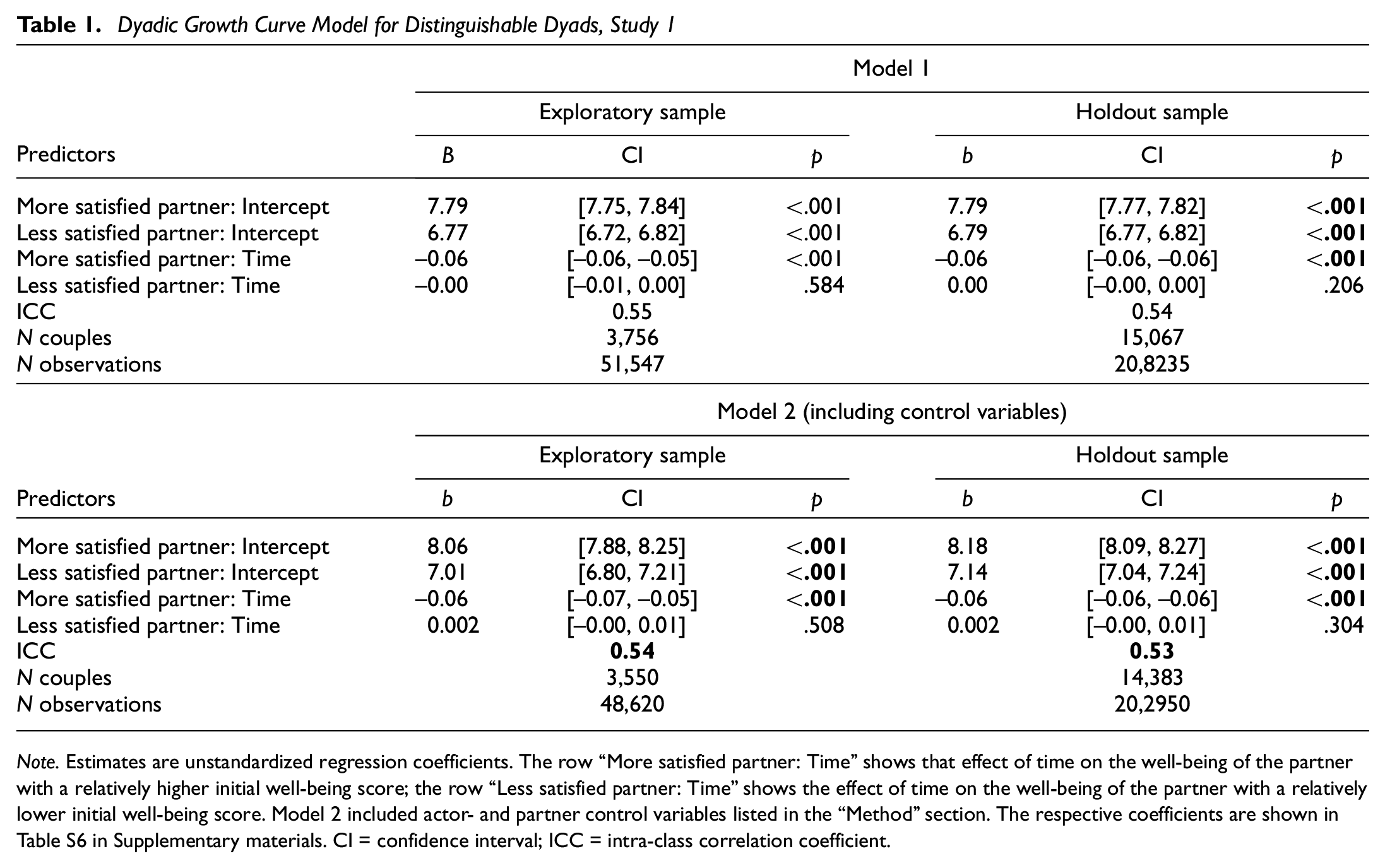
Note. Estimates are unstandardized regression coefficients. The row “More satisfied partner: Time” shows that effect of time on the well-being of the partner with a relatively higher initial well-being score; the row “Less satisfied partner: Time” shows the effect of time on the well-being of the partner with a relatively lower initial well-being score. Model 2 included actor- and partner control variables listed in the “Method” section. The respective coefficients are shown in Table S6 in Supplementary materials. CI = confidence interval; ICC = intra-class correlation coefficient.

In Model 1, for the partner with a higher life satisfaction at baseline, the effect of time was negative and significant, while for the partner with a lower life satisfaction at baseline, the effect of time was not significant, see Table 1. The effect of time for the more satisfied partner was significantly larger (effect size β = −.21) than the effect of time for the less satisfied partner (effect size β = .01; exploratory sample: z = 20.04, p < .001; holdout sample: z = 40.15, p < .001). As seen in Figure 1, the more satisfied partner in a couple experienced a decrease in life satisfaction, while the less satisfied partner in a couple maintained his or her relatively low level of satisfaction across the years. At the end of the observation period (37 years), the partner who was better off initially experienced a decrease in life satisfaction of 2.22 points (corresponding to 1.26 SD). This decrease in satisfaction was so large that, by the end of the observation period, the more satisfied partner became the less satisfied partner in a couple.

Figure 1

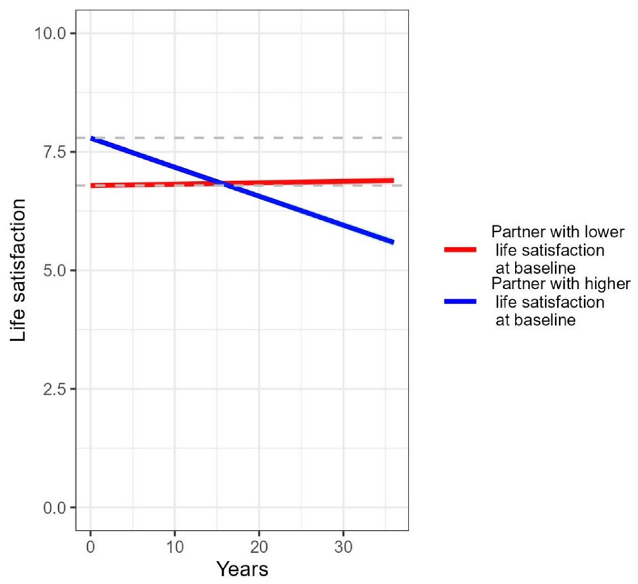
Life Satisfaction Trajectories of as a Function of the Partner’s Relative Standing on Life Satisfaction at Baseline, Study 1

In Model 2, we added the socio-demographic controls as predictors of both partners’ life satisfaction. The effects of time reported above remained unchanged. All coefficients are presented in Table S6 (Supplementary materials).

Altogether, from the results of models both with and without socio-demographic controls, the movement toward similarity of romantic couples can be attributable to a negativity bias—the initially happier partner experienced more dramatic declines in well-being than the initially unhappy partner.

Study 2

Study 2 replicates the negativity bias in well-being co-development in couples in a different national sample—from the Netherlands—and extends it to various indicators of psychological well-being: life satisfaction, positive and negative emotions, and self-esteem.

Method

Participants

We used the data from the Longitudinal Internet Studies for the Social Sciences (LISS Panel). LISS Panel is an annual household panel that consists of a large nationally representative sample of the Dutch population. The panel started in 2008 and the last wave available at the time of writing was collected in 2022 (note that no data were collected in 2015, resulting in 14 waves). We only used the responses of the household head and their (wedded or unwedded) partner. For individuals who had multiple partnerships during the observation period, we used the data associated with the first partnership that took place during the observation period. Like in Study 1, we excluded couples who reported the same level of well-being at baseline (n of excluded couples varied between 147 and 313 depending on the outcome; analyses for these couples are seen in Table S3 and Table S4).

The final dataset included between 3,112 couples (life satisfaction analyses) and 3,393 couples (positive emotions analyses) who contributed between 5.68 (SD = 4.65; life satisfaction) and 5.75 (SD = 4.59; negative emotions) waves on average. A random 20% constituted the Exploratory Sample, and the remaining 80% constituted the Hold-Out (confirmatory) Sample.

Measures

We included all measures of psychological well-being that were available: Life satisfaction, positive and negative affect, and self-esteem.

Life satisfaction was measured with the Satisfaction with Life Scale (5 items; sample item: “I’m satisfied with my life”; Cronbach’s α: .89–.92, depending on the wave) (Diener et al., 1985). Positive and negative emotions were measured with the Positive and Negative Affect Schedule (PANAS) scale that assessed the intensity of 10 positive and 10 negative emotions (Watson et al., 1988). We computed scales of positive and negative emotions by averaging the respective items (Cronbach’s α for positive emotions was .86–.89 and for negative emotions .93–.94). Finally, self-esteem was measured with a 10-item self-esteem scale (sample item: “I take a positive attitude towards myself”; Cronbach’s α: .85–.94) (Rosenberg, 1979). All well-being indicators were measured using a 7-point scale. All items are shown in Table S7 in the Supplementary Materials.

We included the following socio-demographic control variables: actor gender (male = 1, female = 0), actor and partner age, whether the couple is same-sex or not (1 = same-sex, 0 = heterosexual), marital status (1 = married, 0 = cohabiting), presence of joint children (1 = yes, 0 = no), actor and partner level of education (1 = primary school to 6 = university degree) and actor and partner employment status (three categories: employed, self-employed, retired, unemployed, other). Finally, because basic personality traits represent strong predictors of well-being (Chopik & Lucas, 2019), we added both partners’ Big Five values as additional control variables. The Big Five (agreeableness, extraversion, conscientiousness, emotional stability and openness) were measured with the 50-item set of the International Personality Item Pool (1 = very inaccurate, 5 = very accurate) (Goldberg, 1992). All scales showed adequate to good reliability (Cronbach’s αs between .74 and .91).

Analytic Strategy

Like in Study 1, we used the dyadic growth curve model for distinguishable dyads. We followed the analytic strategy of Study 1 without deviations.

Results

Members of the same couple had similar levels of well-being (rs between .44, life satisfaction, and .22, self-esteem, both ps < .001). Still, the partner with a higher well-being scored substantially higher than the partner with a lower well-being (within a couple) on all four well-being measures, at baseline, see Table 2.

Table 2

Baseline Well-Being, Study 2

Outcome	Higher partner: M (SD)	Lower partner: M (SD)	T	df	p	Cohen’s d
Life satisfaction	5.67 (0.80)	4.74 (1.04)	39.17	5,797.8	<.001	1.00
Self-esteem	6.15 (0.69)	5.18 (0.97)	45.65	5,699.8	<.001	1.15
Positive emotions	5.03 (0.78)	4.04 (0.98)	44.18	6,048.0	<.001	1.11
Negative emotions	2.57 (1.11)	1.60 (0.71)	40.71	5,153.8	<.001	1.05

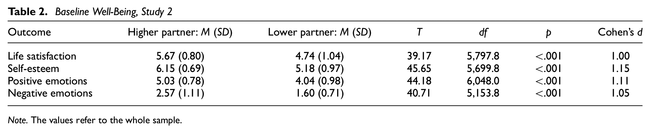
Note. The values refer to the whole sample.

We tested whether the partner with a higher versus lower well-being experienced a greater change in well-being over time using dyadic growth curve models. The results are shown in Table 3 (and in Figure 2). Like in Study 1, the results are nearly identical for both the exploratory and the holdout sample and were not affected by introducing the control variables listed in the “Method” section.

Table 3

Dyadic growth curve model for distinguishable dyads, Study 2

Predictors	Model 1: Exploratory sample
	Life satisfaction			Self-esteem			Positive emotions			Negative emotions
	B	CI	p	b	CI	p	b	CI	p	b	CI	p
Partner w. higher scores: Intercept	5.54	[5.48, 5.60]	<0.001	6.07	[6.01, 6.12]	<0.001	4.89	[4.82, 4.95]	<0.001	2.41	[2.33, 2.49]	<0.001
Partner w. lower scores: Intercept	4.85	[4.78, 4.93]	<0.001	5.27	[5.19, 5.34]	<0.001	4.10	[4.03, 4.17]	<0.001	1.71	[1.66, 1.77]	<0.001
Partner w. higher scores: Time	–0.02	[–0.03, –0.01]	<0.001	–0.02	[–0.03, –0.02]	<0.001	–0.03	[–0.04, –0.02]	<0.001	–0.02	[–0.03, –0.01]	<0.001
Partner w. lower scores: Time	0.01	[0.00, 0.02]	0.038	0.01	[0.00, 0.02]	0.018	0.01	[0.00, 0.02]	0.015	0.03	[0.02, 0.04]	<0.001
ICC	0.74			0.71			0.58			0.47
N couples	615			638			638			606
N observations	6,188			4,881			4,824			4,579
Predictors	Model 1: Holdout sample
	Life satisfaction			Self-esteem			Positive emotions			Negative emotions
	b	CI	p	b	CI	p	b	CI	p	b	CI	p
Partner w. higher scores: Intercept	5.55	[5.52, 5.58]	<0.001	6.08	[6.06, 6.11]	<0.001	4.87	[4.84, 4.90]	<0.001	2.44	[2.40, 2.48]	<0.001
Partner w. lower scores: Intercept	4.84	[4.80, 4.88]	<0.001	5.23	[5.19, 5.26]	<0.001	4.10	[4.07, 4.13]	<0.001	1.70	[1.67, 1.73]	<0.001
Partner w. higher scores: Time	–0.03	[–0.03, –0.02]	<0.001	–0.02	[–0.03, –0.02]	<0.001	–0.03	[–0.03, –0.02]	<0.001	–0.01	[–0.02, –0.01]	<0.001
Partner w. lower scores: Time	0.02	[0.01, 0.02]	<0.001	0.01	[0.00, 0.01]	0.001	0.01	[0.01, 0.02]	<0.001	0.03	[0.02, 0.03]	<0.001
ICC	0.69			0.73			0.56			0.57
N couples	2,476			2,526			2,544			2,425
N observations	24,212			18,706			18,682			17,907
Predictors	Model 2 (including control variables): Exploratory sample
	Life satisfaction			Self-esteem			Positive emotions			Negative emotions
	b	CI	p	b	CI	p	b	CI	p	b	CI	p
Partner w. higher scores: Intercept	5.49	[5.33, 5.65]	<0.001	6.14	[6.02, 6.25]	<0.001	4.85	[4.70, 5.00]	<0.001	2.24	[2.06, 2.42]	<0.001
Partner w. lower scores: Intercept	4.74	[4.56, 4.93]	<0.001	5.37	[5.21, 5.52]	<0.001	4.04	[3.85, 4.22]	<0.001	1.57	[1.41, 1.72]	<0.001
Partner w. higher scores: Time	–0.02	[–0.03, –0.01]	0.001	–0.03	[–0.03, –0.02]	<0.001	–0.03	[–0.04, –0.02]	<0.001	0.00	[–0.01, 0.01]	0.682
Partner w. lower scores: Time	0.01	[0.00, 0.02]	0.020	–0.00	[–0.01, 0.01]	0.559	0.01	[–0.00, 0.02]	0.102	0.03	[0.02, 0.04]	<0.001
ICC	0.65			0.59			0.51			0.35
N couples	606			634			635			603
N observations	4,526			4,808			4,757			4,512
Predictors	Model 2 (including control variables): Holdout sample
	Life satisfaction			Self-esteem			Positive emotions			Negative emotions
	b	CI	p	b	CI	p	b	CI	p	b	CI	p
Partner w. higher scores: Intercept	5.54	[5.46, 5.62]	<0.001	6.07	[6.01, 6.13]	<0.001	4.79	[4.71, 4.87]	<0.001	2.21	[2.12, 2.30]	<0.001
Partner w. lower scores: Intercept	4.88	[4.79, 4.97]	<0.001	5.40	[5.32, 5.47]	<0.001	4.07	[3.98, 4.16]	<0.001	1.63	[1.55, 1.71]	<0.001
Partner w. higher scores: Time	–0.03	[–0.03, –0.02]	<0.001	–0.02	[–0.03, –0.02]	<0.001	–0.02	[–0.03, –0.02]	<0.001	0.00	[–0.00, 0.01]	0.134
Partner w. lower scores: Time	0.01	[0.01, 0.02]	<0.001	–0.00	[–0.01, 0.00]	0.173	0.01	[0.01, 0.02]	<0.001	0.03	[0.03, 0.04]	<0.001
ICC	0.61			0.59			0.49			0.39
N couples	2,444			2,515			2,533			2,414
N observations	17,788			18,497			18,479			17,701

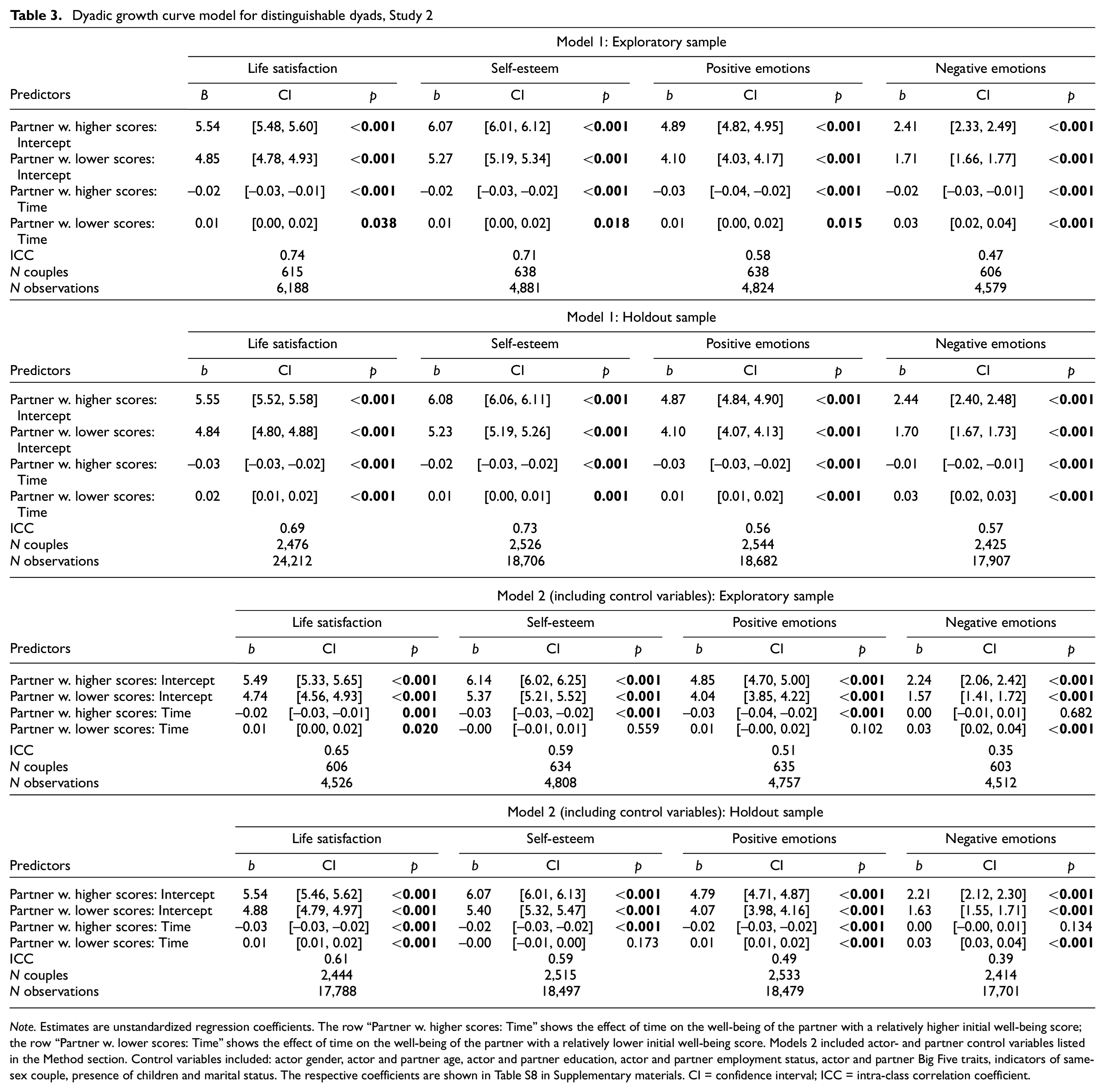
Note. Estimates are unstandardized regression coefficients. The row “Partner w. higher scores: Time” shows the effect of time on the well-being of the partner with a relatively higher initial well-being score; the row “Partner w. lower scores: Time” shows the effect of time on the well-being of the partner with a relatively lower initial well-being score. Models 2 included actor- and partner control variables listed in the Method section. Control variables included: actor gender, actor and partner age, actor and partner education, actor and partner employment status, actor and partner Big Five traits, indicators of same-sex couple, presence of children and marital status. The respective coefficients are shown in Table S8 in Supplementary materials. CI = confidence interval; ICC = intra-class correlation coefficient.

Figure 2

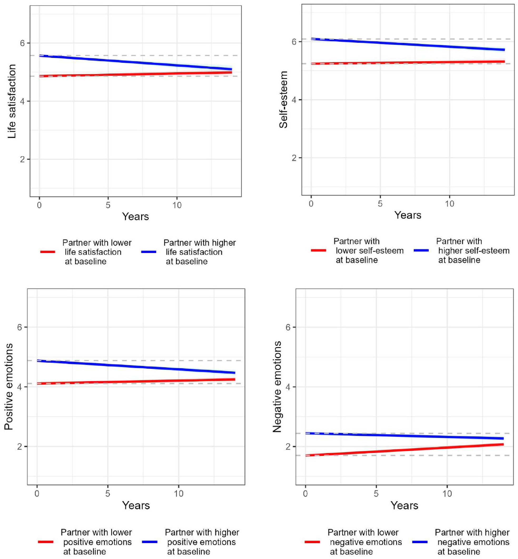
Well-Being Trajectories of Partners With Higher and Lower Initial Well-Being in a Couple at Baseline, Study 2 (Holdout Sample)

For all well-being indicators, the partner with better initial well-being deteriorated over time, while the partner with worse initial well-being improved over time, see Figure 2. Comparing the absolute value of experienced change for both partners using a z-test showed that the well-being deterioration experienced by the partner with the higher initial well-being (higher life satisfaction, higher positive affect, higher self-esteem, lower negative affect) was significantly larger (effect size β .|10|–.|11|) than the improvement experienced by the partner with the lower initial well-being (lower life satisfaction, lower positive affect, lower self-esteem, and higher negative affect; effect size β between .|03| and .|06|). Across all models (with and without control variables, four well-being indicators) and samples (exploratory and holdout), out of 16 comparisons, the difference was significant for 13 comparisons (3 ps > .05, 4 ps < .05 and 9 ps < .001). For example, by the end of the observation period (14 years), the partner with initially higher positive affect is predicted to decrease by .41 points, while the partner with initially lower positive affect is expected to increase only by .14 points. A similar asymmetry is observed for negative emotions: The partner with initially lower negative affect is predicted to increase by .38 points, while the partner with initially higher negative affect is expected to decrease only by .17 points.

An overview of the effect of time on well-being of partners with a lower and a higher baseline well-being for all measures in both studies is shown in Figure 3.

Figure 3

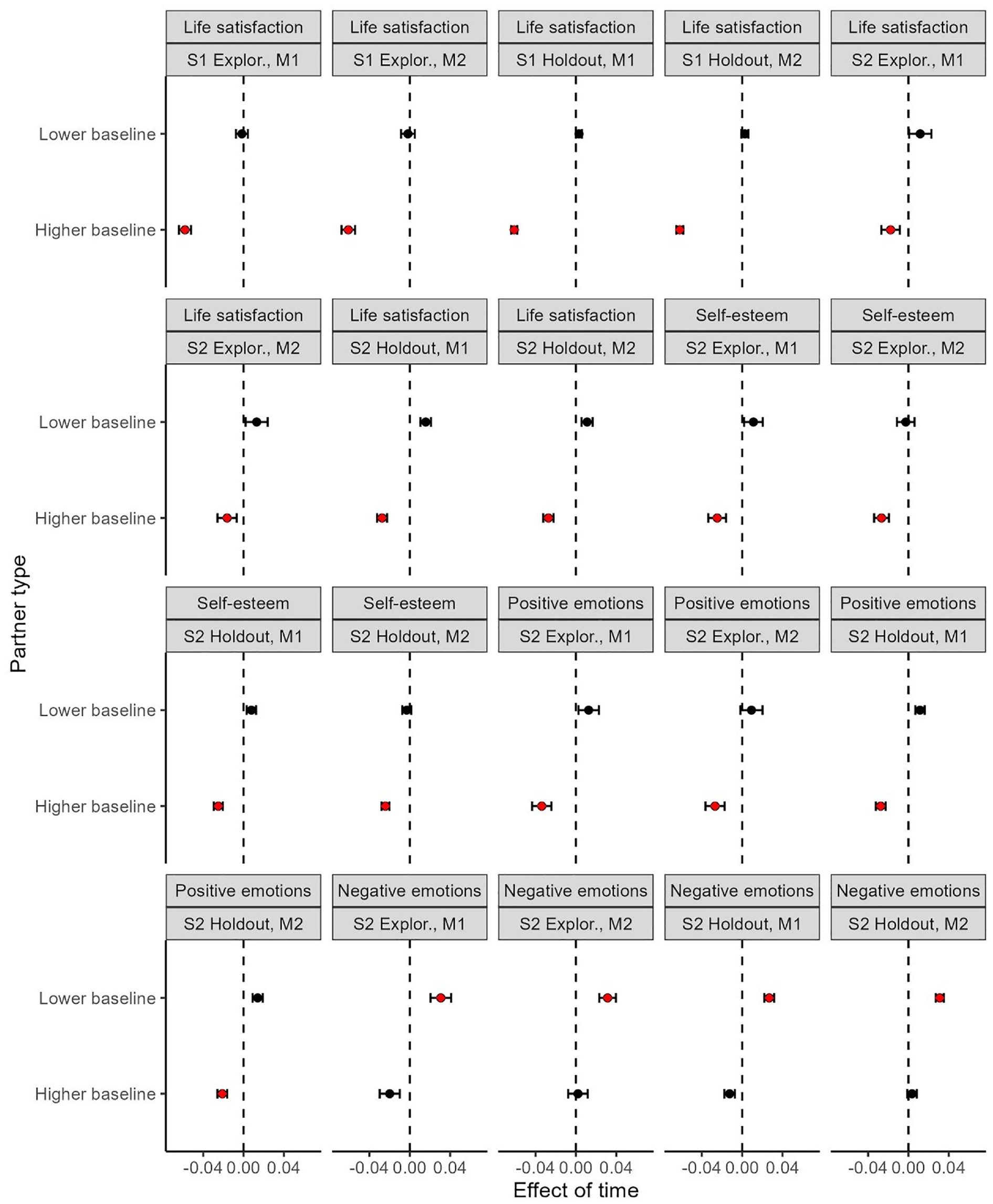
Effect of Time on Well-Being of Partners With a Lower and a Higher Baseline Well-Being

True Change or a Statistical Artifact?

To examine whether our effects reflected true change or ostensibly related statistical artifacts, we ran two robustness checks. First, we explored whether the valence asymmetry—a stronger decline in well-being in the more (vs. less) satisfied partner—could be a result of individuals with higher initial scores (regardless of their standing relative to their partner) showing a steeper decline in well-being over time compared with those with lower initial scores (i.e., they “have nowhere to go but down”). However, the results showed the opposite pattern: Individuals with lower (vs. higher) well-being at baseline on average experienced a stronger change over time (an increase), see Figures S1 (for analysis details, see Supplementary materials). This is at odds with the possibility that the steeper decline of a happier partner in a couple is due to their higher baseline well-being. Furthermore, adding individual’s baseline well-being score as a control variable to the two-intercept model in the main analyses did not change the model coefficients (see Table S9). We conclude that the potential association between individuals’ own baseline well-being and slope cannot explain the negativity bias pattern in the couple co-development presented here.

Second, we explored whether valence asymmetry is attributable to a regression to the mean. Individuals’ particularly high or low scores at baseline could reflect a larger measurement error (rather than true scores), which might not be there at subsequent measurements, creating the illusion of well-being decline or increase. Following Barnett et al. (2004), we used an average of well-being scores at the first three measurement occasions (instead of just the first one) as indicators of baseline well-being. With this approach, individuals’ baseline well-being is less likely to be artificially inflated due to random measurement error and any subsequent change is less likely to reflect a regression to the mean. The results of these analyses are nearly identical to the ones presented in the “Results” section (see Table S10). We conclude that the pattern of change exhibited by partners with a higher versus lower baseline well-being is unlikely to be due to the regression to the mean.

General Discussion

Researchers have observed a cross-over of affective experiences and a notable similarity in psychological well-being in romantic partners. We explored whether the partner similarity is marked by the happier partner’s over-time deterioration or by the less happy partner’s over-time improvement. In two longitudinal studies of over 20,000 couples, the well-being decline experienced by the originally better-off partner was stronger than any well-being improvement experienced by the originally worse-off partner. In short, bad seems to be stronger than good in shaping the dynamics of well-being changes in couples.

Why is the well-being of a happy partner more “fragile” and malleable than the ill-being of the unhappy partner? Consistent with the research on the negativity bias in social and cognitive psychology (Rozin & Royzman, 2001), “negativity” more easily crosses over from one person to the next via social interactions. People frequently share information about stressful or upsetting daily events with their partners as a coping strategy (Barasch, 2020). Disclosing one’s worries and struggles is a prerequisite to receiving social support. Disclosure of negative information might be more powerful in its consequences. Negative information is often given a higher weight in people’s overall affective experiences and decision-making (Baumeister et al., 2001; Rozin & Royzman, 2001). This negativity bias might grant the unhappier partner more power in shaping the couple’s interactions and overall affective experience, letting negativity dominate couples’ daily conversations. This might render unhappiness more “contagious” than happiness, creating a pattern where—over the years—the less happy partner “is dragging down” the happier one.

Limitations and Extensions

Although our two studies had many strengths, they did not provide us with the means to ascertain that the observed changes result from mutual influence or daily interactions and communication patterns between partners where the unhappy partner sets the tone. For example, it is possible the less happy partner is just more likely to experience negative life events (e.g., job loss, health problems) with consequences for the couple as a whole (e.g., one partner’s unemployment negatively affecting household income). Indeed, lower psychological well-being is associated with worse outcomes across different areas of life (Luhmann et al., 2013; Stavrova & Luhmann, 2016), and negative life events experienced by one partner are associated with well-being changes in the other partner too (Luhmann et al., 2014). Hence, studies taking a closer look at partners’ daily interactions using diary, experience sampling, or observational designs might pinpoint whether the patterns and content of daily conversations and behaviors can help explain the stronger sway of unhappiness.

Furthermore, our focus on the couples where the partners differed in well-being at first assessment resulted in the exclusion of a substantial number of couples who had a similar well-being level. Seeking to be more inclusive, in the additional analyses, to determine the partners’“relative happiness position,” we used the first assessment where the initially equally happy partners diverged (instead of the study baseline). These analyses again showed that the deterioration of the happier partner was larger than any improvement of the less happy partner (see Table S4). These observations suggest that sometimes partners with initially equal well-being will diverge/become more different and sometimes partners with initially different well-being will converge and become more similar over time. Our results showed that, regardless of how the differences between partners emerged in the first place, the process of convergence is marked by a negativity bias, that is, a stronger well-being decrease of the initially happier partner. Future studies might explore whether the process of divergence (i.e., where initially similar partners become different) is marked by a similar valence asymmetry (Wortman & Lucas, 2016).

Finally, our findings were agnostic to whether valence asymmetry in well-being co-development in couples might be functional. For example, similarity among spouses has been argued to foster mutual understanding, cohesion, and to provide a common lens through which to view the world and others. Consequently, well-being similarity has been associated with more relationship stability (Finn et al., 2020; Guven et al., 2012; Schade et al., 2016; Wortman & Lucas, 2016). This raises an exciting question of whether the well-being decrease experienced by the initially happier partners might have a beneficial side effect of promoting partner similarity and thus increasing relationship closeness and longevity.

Contributions and Conclusions

The present findings contribute to several streams of the psychological research. First, our contribution pertains to the literature on spousal similarity. There exists wide consensus regarding the existence of partner similarity in well-being levels (i.e., partners are more similar to each other than strangers) and changes over time (i.e., partners show similar over-time fluctuations in well-being). However, there is less agreement regarding over-time convergence in well-being (i.e., the gap in well-being between partners becomes smaller over time). For example, some studies suggest the gap in well-being between relationship partners decreases over time (Anderson et al., 2003; Gonzaga et al., 2007), while other studies reported the gap remains constant or even increases over time (Caspi et al., 1992; Gerstorf et al., 2013; Schade et al., 2016). Our results might help reconcile these findings by showing that a lack of change in the gap (i.e., absolute difference in well-being) might conceal potential directional changes where the happier partner becomes the less happy partner in a couple (like in Study 1).

Furthermore, we add to the research on valence asymmetry in cognitive and social psychology, in particular the negativity bias. For example, our results are consistent with studies on moral contagion (Rozin & Nemeroff, 2002; Stavrova et al., 2016). In this literature, the belief in negative (vs. positive) qualities crossing over from persons to objects is substantially stronger, making the negativity bias an integral part of the concept of moral contagion. Our results suggest that the negativity bias is not exclusive to moral contagion, but likely extends to the phenomenon of emotional contagion—at least with respect to the patterns of long-term well-being development in couples. Finally, we add to the literature on the consequences of psychological well-being. Multiple studies have shown happiness to have positive outcomes for individuals themselves and for their close ones (e.g., partners) in terms of career, health, and longevity (Chopik & O’Brien, 2017; Stavrova, 2019). We add a potentially important qualifier to these findings showing that, although the benefits of happiness might seem uncontested, exceeding one’s partner’s happiness might ultimately give rise to unhappiness over time.

Supplemental Material

sj-docx-1-spp-10.1177_19485506231207673 – Supplemental material for Don’t Drag Me Down: Valence Asymmetry in Well-Being Co-Development in Couples

Supplemental material, sj-docx-1-spp-10.1177_19485506231207673 for Don’t Drag Me Down: Valence Asymmetry in Well-Being Co-Development in Couples by Olga Stavrova and William J. Chopik in Social Psychological and Personality Science

Footnotes

Handling Editor: Jennifer Bosson

Declaration of Conflicting Interests

The author(s) declared no potential conflicts of interest with respect to the research, authorship, and/or publication of this article.

Funding

The author(s) received no financial support for the research, authorship, and/or publication of this article.

ORCID iD

Olga Stavrova

Supplemental Material

Supplemental material for this article is available online.

Notes

Author Biographies

Olga Stavrova is a professor at the University of Lübeck in Germany. She studies subjective well-being, cynicism and trust and interpersonal relationships.

William J. Chopik, PhD, is an associate professor at Michigan State University. He studies the continuity and change of relationship processes across the lifespan and individual differences in responses to intimacy.

References

Anderson

Keltner

John

O. P.

(2003). Emotional convergence between people over time. Journal of Personality and Social Psychology, 84(5), 1054–1068. https://doi.org/10.1037/0022-3514.84.5.1054

Barasch

(2020). The consequences of sharing. Current Opinion in Psychology, 31, 61–66. https://doi.org/10.1016/j.copsyc.2019.06.027

Barnett

A. G.

van der Pols

J. C.

Dobson

A. J.

(2004). Regression to the mean: What it is and how to deal with it. International Journal of Epidemiology, 34(1), 215–220. https://doi.org/10.1093/ije/dyh299

Barsade

S. G.

Coutifaris

C. G.

Pillemer

(2018). Emotional contagion in organizational life. Research in Organizational Behavior, 38, 137–151.

Baumeister

R. F.

Bratslavsky

Finkenauer

Vohs

K. D.

(2001). Bad is stronger than good. Review of General Psychology, 5(4), 323–370. https://doi.org/10.1037/1089-2680.5.4.323

Bebbington

MacLeod

Ellison

T. M.

Fay

(2017). The sky is falling: Evidence of a negativity bias in the social transmission of information. Evolution and Human Behavior, 38(1), 92–101. https://doi.org/10.1016/j.evolhumbehav.2016.07.004

Butner

Diamond

L. M.

Hicks

A. M.

(2007). Attachment style and two forms of affect coregulation between romantic partners. Personal Relationships, 14(3), 431–455.

Caspi

Herbener

E. S.

Ozer

D. J.

(1992). Shared experiences and the similarity of personalities: A longitudinal study of married couples. Journal of Personality and Social Psychology, 62(2), 281–291.

Cheung

Lucas

(2014). Assessing the validity of single-item life satisfaction measures: Results from three large samples. Quality of Life Research, 233, 2809–2818. https://doi.org/10.1007/s11136-014-0726-4

10.

Chopik

W. J.

Lucas

R. E.

(2019). Actor, partner, and similarity effects of personality on global and experienced well-being. Journal of Research in Personality, 78, 249–261. https://doi.org/10.1016/j.jrp.2018.12.008

11.

Chopik

W. J.

O’Brien

(2017). Happy you, healthy me? Having a happy partner is independently associated with better health in oneself. Health Psychology, 36(1), 21–30. https://doi.org/10.1037/hea0000432

12.

Diener

Emmons

R. A.

Larsen

R. J.

Griffin

(1985). The Satisfaction with Life Scale. Journal of Personality Assessment, 49, 71–75.

13.

Diener

Kanazawa

Suh

E. M.

Oishi

(2014). Why people are in a generally good mood. Personality and Social Psychology Review, 19, 235–256. https://doi.org/10.1177/1088868314544467

14.

Diener

Suh

Lucas

Smith

(1999). Subjective well-being: Three decades of progress. Psychological Bulletin, 125(2), 276–302.

15.

Finn

Johnson

M. D.

Neyer

F. J.

(2020). Happily (n) ever after? Codevelopment of romantic partners in continuing and dissolving unions. Developmental Psychology, 56(5), 1022.

16.

Garcia

(2018). Dyadic growth curve modelling. https://randilgarcia.github.io/week-dyad-workshop/Growth_Curve_Modeling.html#dyadic_growth_curve_modeling

17.

Gerstorf

Windsor

T. D.

Hoppmann

C. A.

Butterworth

(2013). Longitudinal change in spousal similarities in mental health: Between-couple and within-couple perspectives. Psychology and Aging, 28(2), 540–554.

18.

Goldberg

L. R.

(1992). The development of markers for the Big-Five factor structure. Psychological Assessment, 4(1), 26–42. https://doi.org/10.1037/1040-3590.4.1.26

19.

Gonzaga

G. C.

Campos

Bradbury

(2007). Similarity, convergence, and relationship satisfaction in dating and married couples. Journal of Personality and Social Psychology, 93(1), 34–48.

20.

Guven

Senik

Stichnoth

(2012). You can’t be happier than your wife. Happiness gaps and divorce. Journal of Economic Behavior & Organization, 82(1), 110–130. https://doi.org/10.1016/j.jebo.2012.01.003

21.

Hatfield

Cacioppo

J. T.

Rapson

R. L.

(1993). Emotional contagion. Current Directions in Psychological Science, 2(3), 96–99. http://search.ebscohost.com/login.aspx?direct=true&db=psyh&AN=1994-05473-001&site=ehost-live

22.

Hicks

A. M.

Diamond

L. M.

(2008). How was your day? Couples’ affect when telling and hearing daily events. Personal Relationships, 15(2), 205–228. https://doi.org/10.1111/j.1475-6811.2008.00194.x

23.

Hoppmann

C. A.

Gerstorf

Willis

S. L.

Schaie

K. W.

(2011). Spousal interrelations in happiness in the Seattle Longitudinal Study: Considerable similarities in levels and change over time. Developmental Psychology, 47(1), 1–8.

24.

Humbad

M. N.

Donnellan

M. B.

Iacono

W. G.

McGue

Burt

S. A.

(2010). Is spousal similarity for personality a matter of convergence or selection? Personality and Individual Differences, 49(7), 827–830. https://doi.org/10.1016/j.paid.2010.07.010

25.

Jackson

S. E.

Steptoe

Wardle

(2015). The influence of partner’s behavior on health behavior change: The English Longitudinal Study of Ageing. JAMA Internal Medicine, 175(3), 385–392. https://doi.org/10.1001/jamainternmed.2014.7554

26.

Joseph

D. L.

Chan

M. Y.

Heintzelman

S. J.

Tay

Diener

Scotney

V. S.

(2020). The manipulation of affect: A meta-analysis of affect induction procedures. Psychological Bulletin, 146(4), 355–375.

27.

Kane

A. A.

van Swol

L. M.

Sarmiento-Lawrence

I. G.

(2023). Emotional contagion in online groups as a function of valence and status. Computers in Human Behavior, 139, 107543. https://doi.org/10.1016/j.chb.2022.107543

28.

Katz

Beach

S. R.

Joiner

T. E.

Jr (1999). Contagious depression in dating couples. Journal of Social and Clinical Psychology, 18(1), 1–13.

29.

Kenny

D. A.

Kashy

D. A.

(2011). Dyadic data analysis using multilevel modeling. In Hox

Kyle Roberts

(Eds.), Handbook for advanced multilevel analysis (pp. 335–370). Routledge/Taylor & Francis Group.

30.

Kenny

D. A.

Kashy

D. A.

Cook

W. L.

(2006). Dyadic data analysis. Guilford Press.

31.

Kiley Hamlin

Wynn

Bloom

(2010). Three-month-olds show a negativity bias in their social evaluations. Developmental Science, 13(6), 923–929.

32.

Kramer

A. D. I.

Guillory

J. E.

Hancock

J. T.

(2014). Experimental evidence of massive-scale emotional contagion through social networks. PNAS Proceedings of the National Academy of Sciences of the United States of America, 111(24), 8788–8790. http://search.ebscohost.com/login.aspx?direct=true&db=psyh&AN=2014-27763-002&site=ehost-live

33.

Luhmann

Lucas

R. E.

Eid

Diener

(2013). The prospective effect of life satisfaction on life events. Social Psychological and Personality Science, 4(1), 39–45. https://doi.org/10.1177/1948550612440105

34.

Luhmann

Weiss

Hosoya

Eid

(2014). Honey, I got fired! A longitudinal dyadic analysis of the effect of unemployment on life satisfaction in couples. Journal of Personality and Social Psychology, 107(1), 163–180. https://doi.org/10.1037/a0036394

35.

Luo

(2017). Assortative mating and couple similarity: Patterns, mechanisms, and consequences. Social and Personality Psychology Compass, 11(8), Article e12337. https://doi.org/doi:10.1111/spc3.12337

36.

Meyler

Stimpson

J. P.

Peek

M. K.

(2007). Health concordance within couples: A systematic review. Social Science & Medicine, 64(11), 2297–2310. https://doi.org/10.1016/j.socscimed.2007.02.007

37.

Nestler

Grimm

K. J.

Schönbrodt

F. D.

(2015). The social consequences and mechanisms of personality: How to analyse longitudinal data from individual, dyadic, round-robin and network designs. European Journal of Personality, 29(2), 272–295. https://doi.org/10.1002/per.1997

38.

Orth

Erol

R. Y.

Ledermann

Grob

(2018). Codevelopment of well-being and self-esteem in romantic partners: Disentangling the effects of mutual influence and shared environment. Developmental Psychology, 54(1), 151–166. https://doi.org/10.1037/dev0000400

39.

Rosenberg

(1979). Conceiving the self. Basic Book.

40.

Rozin

Nemeroff

(2002). Sympathetic magical thinking: The contagion and similarity “heuristics.” In Gilovich

Griffin

Kahneman

(Eds.), Heuristics and biases. The psychology of intuitive judgment (pp. 201–216). Cambridge University Press.

41.

Rozin

Royzman

E. B.

(2001). Negativity bias, negativity dominance, and contagion. Personality and Social Psychology Review, 5(4), 296–320. https://doi.org/10.1207/S15327957PSPR0504_2

42.

Rusconi

Sacchi

Brambilla

Capellini

Cherubini

(2020). Being honest and acting consistently: Boundary conditions of the negativity effect in the attribution of morality. Social Cognition, 38(2), 146–178.

43.

Sakaluk

J. K.

(2016). Exploring small, confirming Big: An alternative system to the new statistics for advancing cumulative and replicable psychological research. Journal of Experimental Social Psychology, 66, 47–54. https://doi.org/10.1016/j.jesp.2015.09.013

44.

Saxbe

Repetti

R. L.

(2010). For better or worse? Coregulation of couples’ cortisol levels and mood states. Journal of Personality and Social Psychology, 98(1), 92.

45.

Schade

H. M.

Hülür

Infurna

F. J.

Hoppmann

C. A.

Gerstorf

(2016). Partner dissimilarity in life satisfaction: Stability and change, correlates, and outcomes. Psychology and Aging, 31(4), 327–339.

46.

Schimmack

Lucas

R. E.

(2010). Environmental influences on well-being: A dyadic latent panel analysis of spousal similarity. Social Indicators Research, 98(1), 1–21. http://search.ebscohost.com/login.aspx?direct=true&db=psyh&AN=2010-16288-001&site=ehost-live

47.

Schoebi

(2008). The coregulation of daily affect in marital relationships. Journal of Family Psychology, 22(4), 595–604.

48.

Socio-Economic Panel. (2022). Socio-Economic Panel (SOEP), data for years 1984-2020, SOEP-Core v37, EU edition. https://doi.org/10.5684/soep.core.v37eu

49.

Song

Foo

M.-D.

M. A.

(2008). Mood spillover and crossover among dual-earner couples: A cell phone event sampling study. Journal of Applied Psychology, 93(2), 443–452.

50.

Stavrova

(2019). Having a happy spouse is associated with lowered risk of mortality. Psychological Science, 30(5), 798–803. https://doi.org/10.1177/0956797619835147

51.

Stavrova

Luhmann

(2016). Social connectedness as a source and consequence of meaning in life. The Journal of Positive Psychology, 11(5), 470–479. https://doi.org/10.1080/17439760.2015.1117127

52.

Stavrova

Newman

Kulemann

Fetchenhauer

(2016). Contamination without contact: An examination of intention-based contagion. Judgment and Decision Making, 11(6), 554–571.

53.

Thompson

Bolger

(1999). Emotional transmission in couples under stress. Journal of Marriage and the Family, 61, 38–48.

54.

Trussler

Soroka

(2014). Consumer demand for cynical and negative news frames. The International Journal of Press/Politics, 19(3), 360–379.

55.

Unkelbach

Alves

Koch

(2020). Negativity bias, positivity bias, and valence asymmetries: Explaining the differential processing of positive and negative information. In Gawronski

(Ed.), Advances in experimental social psychology (Vol. 62, pp. 115–187). Academic Press. https://doi.org/10.1016/bs.aesp.2020.04.005

56.

Unkelbach

Koch

Alves

(2019). The evaluative information ecology: On the frequency and diversity of “good” and “bad.” European Review of Social Psychology, 30(1), 216–270.

57.

Vaish

Grossmann

Woodward

(2008). Not all emotions are created equal: The negativity bias in social-emotional development. Psychological Bulletin, 134(3), 383–403.

58.

Watson

Clark

L. A.

Tellegen

(1988). Development and validation of brief measures of positive and negative affect: The PANAS Scale. Journal of Personality and Social Psychology, 54, 1063–1070.

59.

Weber

Hülür

(2021). Affect contagion in daily life is mediated by perceptions of partner affect: An experience-sampling study with older couples. Emotion, 21(8), 1699–1711.

60.

Westman

(2001). Stress and strain crossover. Human Relations, 54(6), 717–752. http://search.ebscohost.com/login.aspx?direct=true&db=psyh&AN=2001-01931-002&site=ehost-live

61.

Westman

(2013). Crossover of positive states and experiences. Stress and Health: Journal of the International Society for the Investigation of Stress, 29(4), 263–265. http://search.ebscohost.com/login.aspx?direct=true&db=psyh&AN=2013-34738-002&site=ehost-live

62.

Wetzel

Huxhold

Tesch-Römer

(2016). Transition into retirement affects life satisfaction: Short- and Long-term development depends on last labor market status and education. Social Indicators Research, 125(3), 991–1009. https://doi.org/10.1007/s11205-015-0862-4

63.

Wortman

Lucas

R. E.

(2016). Spousal similarity in life satisfaction before and after divorce. Journal of Personality and Social Psychology, 110(4), 625–633.

64.

Wünsche

Weidmann

Grob

(2020). Until death do us part: The codevelopment of life satisfaction in couples preceding the death of one partner. Journal of Personality and Social Psychology, 119(4), 881–900. https://doi.org/10.1037/pspi0000228

65.

Youngblood

Stubbersfield

J. M.

Morin

Glassman

Acerbi

(2021, October 26). Negativity bias in the spread of voter fraud conspiracy theory tweets during the 2020 US election. PsyArXiv.

Supplementary Material

Please find the following supplemental material available below.

For Open Access articles published under a Creative Commons License, all supplemental material carries the same license as the article it is associated with.

For non-Open Access articles published, all supplemental material carries a non-exclusive license, and permission requests for re-use of supplemental material or any part of supplemental material shall be sent directly to the copyright owner as specified in the copyright notice associated with the article.

0.00 MB

0.93 MB