Abstract argumentation has proven to be a versatile tool to model and analyze various problems in an argumentative setting. The addition of collective attacks syntactically extends Dung’s original argumentation frameworks (AFs), while retaining the most desirable properties—the resulting class of frameworks is called SETAFs. While most reasoning tasks in the realm of abstract argumentation have been shown to be intractable, real-world instances oftentimes are not entirely random but admit a certain structure that allows for efficient computational shortcuts. In certain cases, we can characterize this structure via an integer parameter, and exploit these insights with advanced algorithmic techniques. A thorough analysis of the computational aspects of SETAFs w.r.t. parameterized algorithms has not yet been conducted. We start the investigation of these approaches by applying the backdoor and treewidth approaches to SETAFs. A backdoor is a part of a problem instance, such that removing the backdoor leads to a simple structure. If we can find such a backdoor and guess the solution on this part (respectively, extensions), the rest of the solution follows almost effortlessly. Similarly, the treewidth of a problem instance is a parameter that characterizes the properties of the instance’s graph structure. Intuitively, the lower the treewidth of a graph, the more “tree-like” it is. Since most argumentation problems become easy on trees, one can exploit low treewidth for efficient algorithms. In this paper, we establish that for SETAFs with constant backdoor sizes general argumentation tasks become efficiently solvable—they are fixed-parameter tractable. We generalize the respective techniques that are known for the special case of Dung-style AFs and show that they also apply to the more general case of SETAFs. In addition, we can show an improvement in the asymptotic runtime compared to earlier approaches for AFs via two-valued guesses instead of the state-of-the-art three-valued approach. Along the way, we point out similarities and interesting situations arising from the more general setting. While treewidth is well-studied in the context of AFs with their graph structure, it cannot be directly applied to the (directed) hypergraphs representing SETAFs. We thus introduce two generalizations of treewidth based on different graphs that can be associated with SETAFs, that is, the primal graph and the incidence graph. We show that while some of these notions allow for parameterized tractability results, reasoning remains intractable for other notions, even if we fix the parameter to a small constant. We present parameterized algorithms for efficient reasoning on SETAFs via tree decompositions by characterizing extensions not only by labeling the arguments, but also by assigning (temporary) labels to the attacks.
In the last few decades of argumentation research, several formalizations have been considered for suitable abstractions of argumentation processes—Dung’s approach of abstract argumentation frameworks (AFs)1 is nowadays one of the most widely used such formalisms. In AFs, arguments are abstract entities represented by nodes in a directed graph, the edges form the attack relation. Several generalizations have been proposed in order to achieve more expressiveness or to be able to instantiate knowledge bases more easily or intuitively. It turned out that, in particular, the binary attack relation of AFs occasionally limits the expressiveness of frameworks, if one is not willing to introduce artificial arguments to model technicalities. One such generalization is the addition of collective attacks2: If a set S collectively attacks an argument, said argument is only effectively defeated by S if all arguments in S are accepted by an agent. The resulting class of frameworks is referred to as SETAFs. Due to SETAFs being highly expressive yet intuitive, there is now an increased interest in this formalism within the research community.
Reasoning in AFs is computationally expensive—in order to still obtain efficient runtimes in special cases restrictions of the graph structure have been investigated.3–5 While, in the general case, the same (mostly intractable) complexity upper bounds hold for SETAFs,6 tractable graph classes have only recently been brought to the attention of the research community.7–10 A particular challenge hereby is to extend structural parameters (that work well for the simple structure of AFs), to the hypergraph structure SETAFs provide. In fact, it turned out that while for certain generalizations the parameterized tractability results of AFs carry over to SETAFs, other scenarios give rise to interesting behavior that leads to most problems remaining intractable.
In this paper, we use the tools of parameterized complexity analysis and focus on two parameters, namely (1) minimum-size deletion-backdoors and (2) treewidth.
The backdoor concept is used in different contexts such as constraint satisfaction problems, satisfiability checking (SAT), answer set programming (ASP) (see e.g. Gaspers et al.,11,12 Fichte and Szeider,13 and Ordyniak et al.14 for recent work), and has also been investigated in the context of AFs.15 Intuitively, a backdoor is one part of an instance that “makes it hard to solve.” In this work, we focus on deletion-backdoors, that is, if this backdoor is removed from the instance, the remaining (sub-)instance is computationally easy. In the context of formal argumentation, this means that a framework belongs to a tractable class (such as acyclicity) after removing certain arguments. This means we can utilize the tractability results of these easy classes for general frameworks without restrictions, as arbitrary distances to the tractable fragments are allowed. If this distance is small (constant), we can reason in polynomial time.15
A low treewidth indicates a certain “tree-likeness” of a graph, and as problems often become easy on trees, adapted versions of these easy algorithms can often be applied to instances with low treewidth. In AFs, it has been shown that reasoning is indeed fixed-parameter tractable w.r.t. treewidth.16–20 Also, in the field of structured argumentation, the parameter treewidth has recently been investigated w.r.t. assumption-based argumentation by Popescu and Wallner,21 who show fixed-parameter tractability for several reasoning problems via monadic second-order logic and tailored algorithms, similarly to the work we present in this paper. We investigate how this notion of treewidth is applicable to the directed hypergraph structure of SETAFs and show that certain generalizations admit fixed-parameter tractability () algorithms, while other reasonable attempts do not.
We want to highlight why these two parameters are a natural choice for the start of a parameterized analysis of the computational properties of SETAFs: backdoor-size and treewidth are orthogonal, that is, there are SETAFs that have low treewidth but arbitrarily large backdoor-sets, and SETAFs with small backdoors but high treewidth. This follows from a corresponding result from AFs.22 For AFs, also the hybrid parameter backdoor–treewidth has been investigated, which guarantees a parameter value that dominates both backdoor size and treewidth, at the cost of a more intricate process to compute the actual parameter value.22
We first recall the necessary preliminaries in Section 2. Our main contributions are as follows:
In Section 3, we present the graph notions necessary for our algorithms and discuss the additional considerations needed for SETAFs’ hypergraphs compared to the simple graph structure of AFs. Moreover, we introduce the concept of deletion-backdoors for SETAFs utilizing the concept of primal-graphs for SETAFs,10 and recall the notion of treewidth.
Section 4 then introduces an algorithm to reason w.r.t. the common admissibility-based semantics of complete, stable, preferred, and semi-stable extensions that exploits given backdoors for the fragments acyclicity and even-cycle-freeness (as introduced for SETAFs in Dvořák et al.23), thereby improving the runtime of the best-known backdoor approach for AFs.15
In Section 5, we show that our introduced backdoor algorithm for preferred semantics is optimal unless the strong exponential time hypothesis is false.
In Section 6, we discuss how the idea of the treewidth parameter can be applied in the context of SETAFs. In Section 6.1, we first present negative results regarding primal treewidth, namely that reasoning remains intractable even for small parameter values. Section 6.2 establishes results for incidence treewidth via a generic argument utilizing Monadic second-order logic, indicating that the idea of treewidth is indeed applicable to SETAFs.
In Section 7, we refine and improve the theoretical results of Section 6.2 as we discuss a dynamic programming algorithm tailored to SETAFs for stable, admissible, and complete semantics. We thereby obtain algorithms with faster runtimes and lay the groundwork for similar algorithms for other admissibility-based semantics.
Finally, in Section 8, we conclude and give pointers to possibly interesting directions for future research.
This paper contains and extends the contents of the papers.8,9 In Dvořák et al.,9 we presented the backdoor approach for SETAFs for preferred extensions together with a conditional lower bound. We extend this in this paper by providing detailed proofs, as well as specifically characterizing complete extensions and presenting a speedup for stable semantics. In Dvořák et al.,8 we presented our approach to exploit treewidth for algorithms for reasoning problems in stable semantics. We extend these results by formal proofs of the algorithms’ soundness and completeness, as well as introducing tailor-made algorithms for admissible sets and complete extensions, solving the problem of characterizing undecided arguments and attacks in this setting.
SETAFs and their semantics
In this section, we start by recalling the definition of AFs with collective attacks (SETAFs).2 SETAFs generalize Dung’s AFs,1 where on the set of arguments A we have a binary attack relation . In SETAFs, attacks are between a non-empty set of arguments and a single argument. SETAFs have recently been in the focus of argumentation research, see the literature.10,24–26 With a slight abuse of notation, we identify Dung’s AFs as a special case of SETAFs—the semantics coincide whenever for each attack the set of attacking arguments is a singleton, see, for example, Caminada et al.26
A SETAF is a pair where A is a finite set of arguments, and is the attack relation. For an attack , we call T the tail and h the head of the attack. SETAFs , where for all it holds that , amount to (standard Dung) AFs. In that case, we usually write to denote the set-attack . For , we say Sattacks an argument if there is an attack with . We use to denote the set and define the range of S (w.r.t. R), denoted , as the set . If S attacks a we say that S attacks each s.t. .
The well-known notions of conflict and defense from classical Dung-style AFs naturally generalize to SETAFs. In contrast to AFs, where conflict-free sets contain no adjacent vertices of an AF’s graph, for SETAFs parts of an attack can be within a conflict-free set—as long as some part lies outside the set.
Let be a SETAF. A set is conflicting in if for some . is conflict-free in , if S is not conflicting in , that is, if for each . denotes the set of all conflict-free sets in .
Defense is a central concept in abstract argumentation: the idea of countering every incoming attack. For SETAFs, to be defended against an incoming attack it suffices to counter-attack a single argument —as this means that the set T is attacked. Formally:
Let be a SETAF. An argument is defended (in ) by a set if for each , such that , also in . A set is defended (in ) by S if each is defended by S (in ).
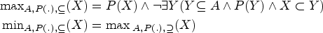
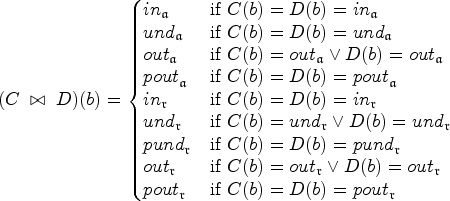
The semantics we study in this work are the admissible, complete, preferred, stable, semi-stable, and stage semantics, which we will abbreviate by , , , , , and , respectively.2,6,25 denotes the set of extensions of under semantics .
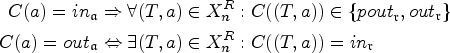
Given a SETAF and a conflict-free set . Then,
, if S defends itself in ,
, if and for all defended by S,
, if and there is no s.t. ,
, if ,
, if and s.t. , and
, if and s.t. .
The relationship between the semantics has been clarified in Dvořák et al.,6 Nielsen and Parsons,2 and Flouris and Bikakis25 and matches with the relations between the semantics for Dung AFs, that is, for any SETAF :
We assume the reader to have basic knowledge in computational complexity theory (For a gentle introduction to complexity theory in the context of formal argumentation, see Dvořák and Dunne24.), in particular, we make use of the complexity classes (polynomial time), (non-deterministic polynomial time), , , and . For a SETAF and an argument , we consider the standard reasoning problems (under semantics ):
Credulous acceptance : Is a contained in at least one extension of ?
Skeptical acceptance : Is a contained in all extensions of ?
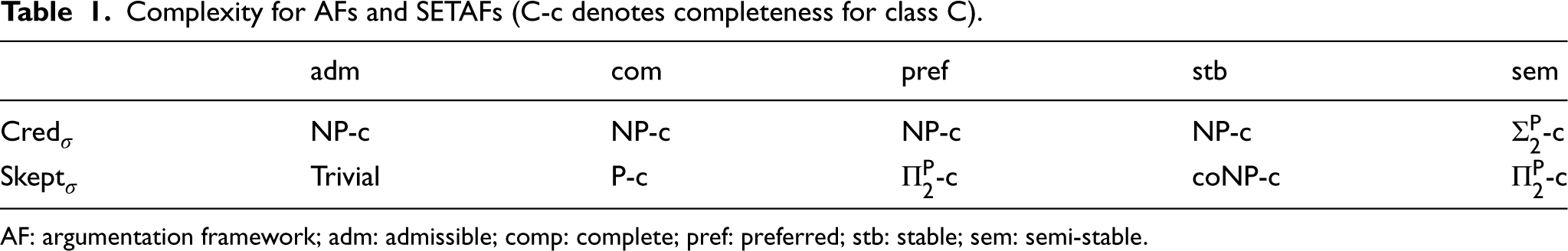
The complexity landscape of SETAFs coincides with that of Dung AFs and is depicted in Table 1. As SETAFs generalize Dung AFs the hardness results for Dung AFs24 carry over to SETAFs, also the same upper bounds hold for SETAFs.6 Note that all complexity results are w.r.t. the total size a SETAF , denoted by , which entails the size of the arguments and the size of the attacks . In contrast to AFs where there can be at most many attacks, in SETAFs, the number of attacks can be exponential in the number of arguments.
Complexity for AFs and SETAFs (-c denotes completeness for class ).
For a more fine-grained complexity analysis, we make use of the complexity class : a problem is fixed-parameter tractable w.r.t. a parameter p if there is an algorithm with runtime , where n is the size of the input, p is an integer (describing certain features of the instance) called the parameter value, and is an arbitrary computable function independent of n (typically at least exponential in p). We also make use of the class . A problem is in w.r.t. a parameter p if there is an algorithm with runtime , where again n is the size of the input and p is the parameter value. We have that . As problems that can be decided in polynomial time are therefore trivially also decidable in , we will in the following not discuss such problems. For example, as the grounded extension (i.e., the unique -minimal complete extension) can be computed in polynomial time, we do not discuss grounded semantics in this paper.
Toward SETAF backdoors
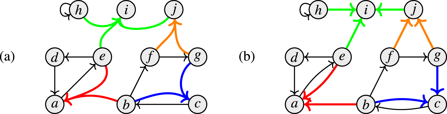
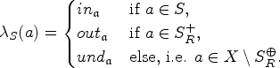
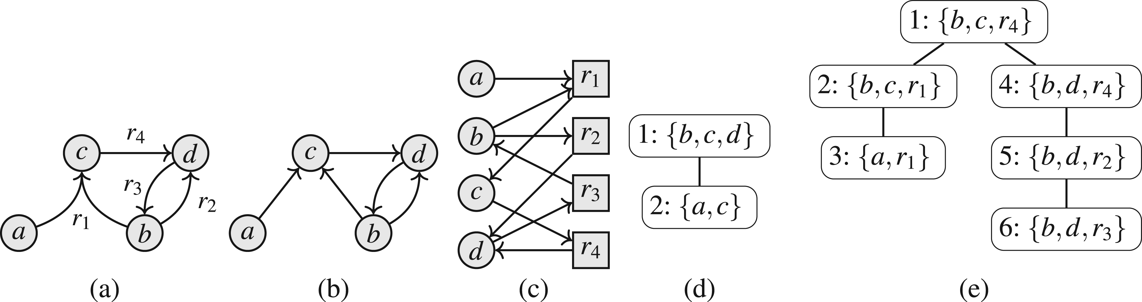
The underlying structure of SETAFs is a directed hypergraph, which makes it hard to apply certain notions of graph properties. We can avoid these issues by utilizing “standard” directed graphs to describe SETAFs and analyze graph properties (such as backdoors and treewidth). There are different such directed graph-representations7,23; we focus on the primal graph, as it arguably is the most intuitive way to embed SETAFs into directed graphs and fits our purposes best. The primal graph has proven useful as a starting point for graph-focused investigations; as such it has been used to investigate the effect of bounded cycle length,7 as well as other graph properties such as (even/odd)-cycle-freeness, bipartiteness, and symmetry.10 An example for a primal graph is given in Figure 1; the corresponding SETAF will serve as a running example for Section 4.
(a) The SETAF and (b) its primal graph . Collective attacks and their corresponding edges in the primal graph are highlighted.
Let be a SETAF. The primal graph of is defined as , where . A (primal-)cycle of length n in is a non-repeating sequence of arguments such that for each there is such that , and there is with . Equivalently, a primal cycle corresponds to a directed cycle in . SETAFs with
no primal cycles are called acyclic, and
no primal cycles of even length are called even-cycle-free.
While for AFs, the primal graph just coincides with the AF itself and therefore uniquely identifies the framework, it is easy to see that several SETAFs can map to the same primal graph. However, restrictions on the primal graph are often useful to obtain computational speedups for otherwise hard problems.7,8,10,23
We denote the classes of acyclic, even-cycle-free SETAFs by , respectively. Note that in the special case of AFs, these classes coincide with the standard definitions, that is, they properly generalize the standard case. For AFs, also the classes of bipartite and symmetric frameworks have been investigated. However, while finding suitable backdoors to these classes was shown to be parameterized-tractable, reasoning in AFs with constant backdoor size to these frameworks remains hard.15 Even though there are generalizations of symmetry and bipartiteness for SETAFs where reasoning also becomes tractable,23 as these classes generalize the respective properties of AFs, the hardness results for backdoor evaluation carry over to the general SETAFs. Hence, we focus on the fragments and . On AFs, all of these classes are considered as the tractable fragments of argumentation, as for many semantics there are efficient algorithms to reason in AFs that belong to one of these classes.3–5 However, these fragments restrict the possible structure of an AF. In order to exploit the speedup while still keeping the full expressiveness, the requirements have been weakened to allow for arbitrary distance to these fragments. We generalize this so-called backdoor approach by Dvořák et al.15 to SETAFs and their hypergraph structure.
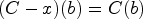
For this, we need the notion of the projection. Intuitively, a SETAF projected to a set of arguments (we write ) can be seen as the result of removing the arguments outside of S while retaining as much of the original structure as possible. This means, for projecting on S (i.e., computing ), we remove all arguments and only keep the arguments in S. Consequently, we also remove all attacks where the head h is not in S, and where the tail T consists only of arguments outside of S (i.e., where the tail would be empty in which is not possible for a SETAF). Moreover, for the remaining attacks, we remove from the tail the arguments outside of S, and retain the attack . In the context of backdoor sets , we project to the set , as we are interested in the remaining framework after removing the backdoor arguments. Formally:
Let be a SETAF and let be a class of SETAFs. We call a set a backdoor if belongs to , where
We denote the size of a smallest backdoor by .
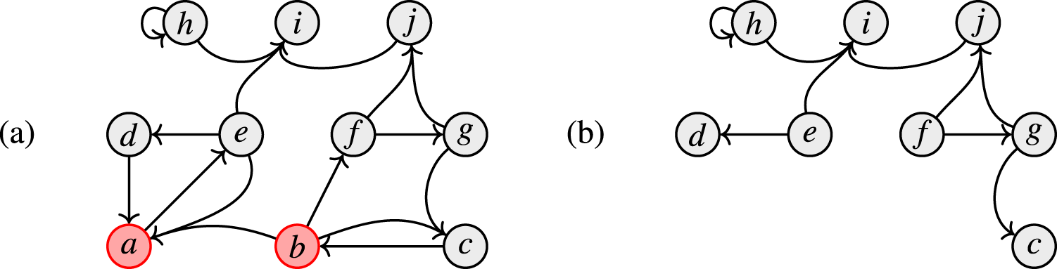
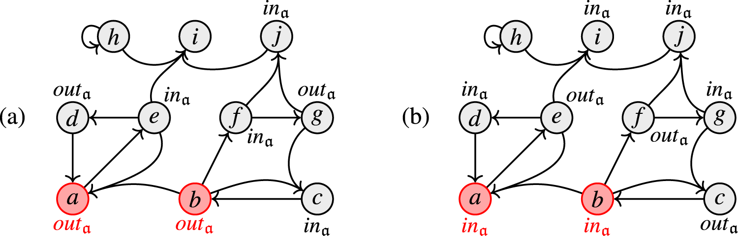
Figure 2 illustrates the idea of backdoors: the set is an backdoor for the SETAF of size 2. It is easy to see in Figure 2(b) that in the SETAF projected to , that is, the remaining framework after removing the backdoor, has no directed cycles of even length in its primal graph. We want to highlight that in the attack from is not deleted as a whole, but “reduced” to the attack . It can easily be verified that indeed, B is the smallest backdoor. For any -backdoor, furthermore the argument h has to be included (in general, every backdoor is a backdoor but not vice versa). Hence, for our example, we have and . While, in this work, we deal with “deletion backdoors” we want to emphasize that the “deletion” step in this workflow is purely conceptual to determine whether a given set S of arguments is indeed a backdoor to the given fragment. The framework is ultimately evaluated as a whole, which distinguishes the backdoor approach from seemingly similar notions where parts of the framework are actually removed such as forgetting.27
It was shown that reasoning in AFs w.r.t. stable, complete, and preferred semantics is tractable for the fragments if is fixed,15 we generalize these results in Section 4. We can efficiently recognize these classes for AFs15 and find backdoors of bounded size. As we defined the fragments for SETAFs on the primal graph, the respective results from AFs (as per Dvořák et al.15) immediately carry over to our setting.
(a) The SETAF with the highlighted backdoor and (b) the “remaining” framework after the deletion of B.
Let be a SETAF.
We can recognize whether belongs to or in polynomial time.
We can find a backdoor of size at most p in time (or if no such backdoor exists correctly detect so).
We can find an backdoor of size at most p in time (or if no such backdoor exists correctly detect so).
This means that the fragment is in principle suitable for algorithms, while for , we aim for algorithms. Note, however, that it is principally possible that faster algorithms for finding backdoors exist.
Backdoor evaluation
In this section, we tackle the evaluation of backdoors of constant size, that is, assume we are given a backdoor, how can we efficiently compute the extensions? We adapt the results from Dvořák et al.15 and generalize the therein-mentioned notions such as partial labelings and propagation algorithms to SETAFs. Our approach, however, differs from the one in Dvořák et al.,15 as it is tailored to the fragments and . This allows us to give a tighter upper bound for the runtime: instead of where p is the size of the given backdoor and n is the size of the instance. Our improved algorithm is applicable to SETAFs as well as AFs, as the latter is just a special case of the former. Note that we put some of the proofs in Appendix A to improve the readability of the paper.
The basic idea of the backdoor evaluation algorithm is to guess parts of an extension on the arguments in the backdoor, and then cleverly propagate this guess to the rest of the instance. As the remaining instance is even-cycle-free, there are no supportive cycles to consider in the propagation step.
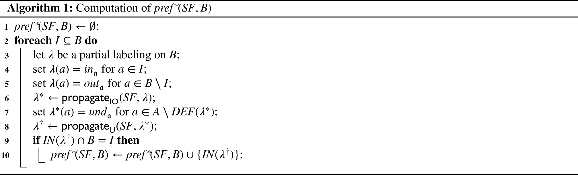
Algorithm 1 captures the whole process to characterize preferred extensions; in Section 4.1, we will verify its correctness and give an intuition for each step. If we provide for a SETAF a backdoor B, Algorithm 1 returns a set of admissible candidates for preferred extensions. In Section 4.2, we show how this algorithm can be sped up for the computation of stable extensions, and in Section 4.3, we generalize the approach of Dvořák et al.15 for complete extensions to SETAFs (note, however, that due to the potential maximal number of complete extensions, it is not possible to obtain the same runtime in this case, instead we provide an time algorithm).
Characterizing preferred extensions
We start with an algorithm to characterize preferred extensions, to which end we first introduce the following technical notions. We capture the concept of the partial guess by partial labelings (cf. Dvořák et al.15).
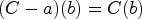
Let be a SETAF and let be a set of arguments. A partial labeling is a function . By we denote the set (similarly, ). We write to identify the set X. For a set we fix the corresponding partial labeling on X as
A labeling is compatible with a set if it holds .
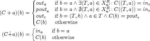
Note that we can use this algorithm also for reasoning problems in other semantics such as complete, stable, or semi-stable with only slight adaptations. We consider two “phases” of propagation. First, we propagate the labels of the guess as far as possible by utilizing the function .
Let be a SETAF and be a partial labeling on . Consider the following propagation rules for :
set if with ,
set if there is a with .
We define as the result of initializing with on , and then exhaustively applying the rules (1) and (2) to each argument .
The second phase fixes incorrectly labeled arguments and assures admissibility in the generated labeling by effectively propagating the label utilizing the function (see Definition 10). We will show that with this approach we can capture all preferred extensions. Following Algorithm 1 we initially label all arguments by that did not get any label during the first phase of applying .
Let be a SETAF and be a partial labeling on . Consider the following propagation rules for :
set if and there is s.t. ,
set if and there is no s.t. .
We define as the result of initializing with on , and then exhaustively applying the rules (3) and (4) to each argument .
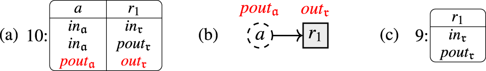
In the following Lemma 11 we formalize the intuition of in the context of Algorithm 1. By applying the function in step 6 we propagate the labels we guessed on B (steps 3–5) and treat them at this stage as if they are “confirmed,” that is, whenever an argument is defended according to the current partial labeling, we add it (by labeling it ), whenever an argument is defeated by the partial labeling, we keep track of this fact (by labeling it ). In this stage, no argument will be labeled . We revisit our running example from Figure 2. Assume we guess for the backdoor . The labeling after exhaustively applying rules (1) and (2) is depicted in Figure 3(a). In general, we will incorrectly label arguments: as can be seen, the argument a is labeled , but there is no attack toward a that verifies this label. Now assume we guess . One can see in Figure 3(b) that there is a problem with the propagated labeling : the arguments d and a are both labeled , effectively causing a conflict. Though we will correct this problem in the second step of the propagation algorithm, we will have to change the label of a from to . We will see that we can actually already stop at this point, as we will then compute (a subset of) the extension we get from the guess . In the following lemma, we establish that for a “correct” guess on the backdoor arguments (i.e., a guess that actually corresponds to a preferred extension E) we label all arguments correctly (i.e., and , respectively).
The first propagation (a) , (b) , on the guessed labels for the backdoor arguments a and b (highlighted).
Let be a SETAF, let , and a NOEVEN backdoor for . For the input to Algorithm 1, assume in step 2 we choose , let be the corresponding partial labeling from steps 4 and 5. Set . Then for each :
if then ,
if then ,
if then ,
, and
.
Next, we illustrate the idea of the function . In particular, it is easy to see that any partial labeling with that we give as input to will give us an admissible set (rule (3) removes conflicts and both rules (3) and (4) resolve undefended arguments).
Let be a SETAF, and let be an arbitrary labeling s.t. . Set . Then is admissible in .
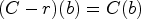
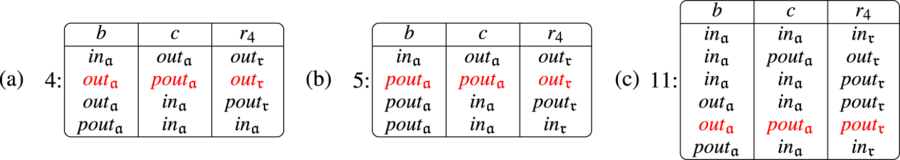
Finally, we show in Lemma 13 that by applying both functions and consecutively, we indeed obtain a preferred extension that corresponds to the guess on B. An argument is incorrectly labeled if it is not defended against each attack; it is incorrectly labeled if it is not attacked from within the set . By exhaustively applying the propagation rules (3) and (4) we fix these incorrect labels. To illustrate this, we revisit our running example. In Figure 3, we see the resulting labelings for the backdoor for the guesses (a) and (b) . Following Algorithm 1, in step 7 we set the arguments without a label to and compute for both labelings. In Figure 4, we see the resulting labelings . Our algorithm outputs the sets , respectively, and it can be indeed verified that these sets are preferred in . Now consider the guess . It turns out that : the fact that both labelings result in the same propagation means in particular that there is no preferred extension E where , as by trying to construct such an extension in (b) we had to correct the label of a. In general, whenever we re-label one of the guessed labels, we can abort the run of the algorithm on this guess and proceed with a different guess, as we will always compute (a superset of) the thereby “missed” set when we start with the corresponding “correct” labeling on the backdoor arguments.
The second propagation (a) , (b) , computed on the labels from Figure 3(a) and (b), respectively.
We show in the following Lemma 13 that for every argument a where we fix the label , a is indeed neither in the corresponding extension nor attacked by it, that is, . This together with the results of Lemma 11 suffices to show that if we guess correctly, the algorithm computes every preferred extension.
Let be a SETAF, let , and a NOEVEN backdoor for . For the input to Algorithm 1, assume in step 2 we choose , let be the corresponding propagated partial labeling from step 7 with labels. Set . Then .
These correctness results for the propagation procedures are the basis for the main result of this section, namely the efficient computation of preferred extensions if a suitable backdoor is given.
Let be a SETAF class, let be a SETAF, and a backdoor for with . With Algorithm 1 we can characterize all extensions in time for on input .
Let , we show that E is in the output of Algorithm 1, that is, . Since in step 2 we try all subsets of B, we will try . Lemma 13 ensures . It remains to show that all steps 3–10 can be done in polynomial time w.r.t. . It is easy to see that (assuming we use reasonable data structures) this is the case for steps 3–5, 7, 9, and 10. For steps 6 and 8 note that each argument is (re)-labeled at most once, and the check for each propagation rule can clearly be carried out in polynomial time. Hence, the overall runtime is . Since , we indeed characterize all stable, semi-stable, and preferred extensions.
Finally, we can then check whether the extensions are (range)-subset-maximal or attack every argument not in them, as all candidates are available. Hence, we can remove those sets that are not preferred/stable/semi-stable. “Filtering out” the stable extensions amounts to checking for each candidate whether the range covers all arguments, which can be done in polynomial time. To actually enumerate all preferred and semi-stable extensions and decide skeptical acceptance, we still have to filter out the solution candidates that are not (range-)subset-maximal. To this end, we can pairwise compare the solution candidates in quadratic runtime w.r.t. the number of solution candidates, which for enumerating and skeptical acceptance gives us a worst-case runtime of .
That is, from the fact that we can compute the candidate set in we immediately get that also preferred and semi-stable extensions can be enumerated in . A similar observation has been made in the AF case.15 However, no details for the exact runtime bounds are provided (In our workshop version of this result,9 we also erroneously do not account for the quadratic time pairwise comparison and instead state an overall runtime of in all cases.). We next provide details on how to enumerate preferred extensions in , which is a significant improvement over the above bound and the bound one would get with the naive approach in the AF setting.15 The key observation here is that when comparing candidate labelings in order to decide whether one induces a superset of the other it suffices to consider the corresponding partial labelings on the backdoor set B. That is, a labeling is a subset of if the corresponding partial labelings , over B satisfy the following:
there is no such that , and ,
there is some such that and , and
there is no such that and .
That is, if one of the candidate labelings sets an argument of the backdoor to and a different candidate labeling sets it to then these two labelings correspond to incomparable sets. We can use this observation to enumerate preferred extensions as follows. First of all, we keep track of all three-valued labelings over the backdoor and indicate its status of whether (1) it is a preferred extension, (2) admissible but a subset of a larger admissible set, (3) no admissible set at all, or (4) not yet considered. Starting with the labelings with no undecided labels, we then iterate over them, test whether they induce a complete extension, and update the corresponding status of the processed candidate, as well as the candidates who have one additional undecided argument and are compatible with the processed candidate (w.r.t. the conditions stated above). If the labeling is complete it is indeed also preferred (case 1) and we add it to the solution set and mark all the successors as superseded by it (case 2). If the set is not admissible at all we simply proceed with the next one (case 3). When done with the labelings with no undecided labels, we apply the same procedure to labelings with one undecided label and then continue by increasing the number of undecided arguments until we end up with the labeling that labels the whole backdoor undecided. The only difference is that we additionally have to check whether the current labeling is already superseded by some other labeling and if so we propagate this status to its successors. Notice that we have such labelings in total, and each solution candidate has at most p successors. That is, the above procedure is in . Regarding semi-stable extensions, notice that the above approach does not work correctly, as it does not suffice to compare the partial labelings on B to compare the ranges of the corresponding extensions. So far, we do not see a way to overcome this even in the AF case, and hence, we only obtain the bound of from the naive approach.
As we can efficiently characterize all preferred extensions, also credulous reasoning becomes efficient in this case. This result also carries over to admissible and complete semantics, as the respective credulous acceptance problems coincide with preferred semantics, is already possible in polynomial time and is trivial. We want to highlight that even if we have a backdoor of size p, there can be up to complete extensions. Clearly we cannot enumerate them with our approach, which is why we capture the preferred extensions (in contrast to the AF approach15).
Let be a SETAF class, let be a SETAF, and a backdoor for with . Then we can decide the problems and in time for . Moreover, we can decide the problems and in time for .
Combining Corollaries 7 and 15, we immediately obtain the following result that captures finding and exploiting minimal backdoors for SETAFs.
Let be a SETAF and let be a semantics.
If , we can solve and in w.r.t. parameter p.
If , we can solve and in w.r.t. parameter p.
In fact, our algorithm for exploiting a small backdoor that is already given is only in for the parameter value p, which is an improvement over the existing approach.15 This also has implications in practice, as it turns out that finding the minimal backdoor size often comes with high computational cost: for example, one known algorithm for the computation of minimal backdoors of size p for directed graphs has runtime ,28 which is often impractical even for rather small parameter values. Instead, recent implementations focus on finding backdoors heuristically, cf. Dvořák et al.22 Note that since our algorithm is directly applicable to AFs and dominates the state-of-the-art approach for AFs, our results are also relevant for the development of fast algorithms for AFs.
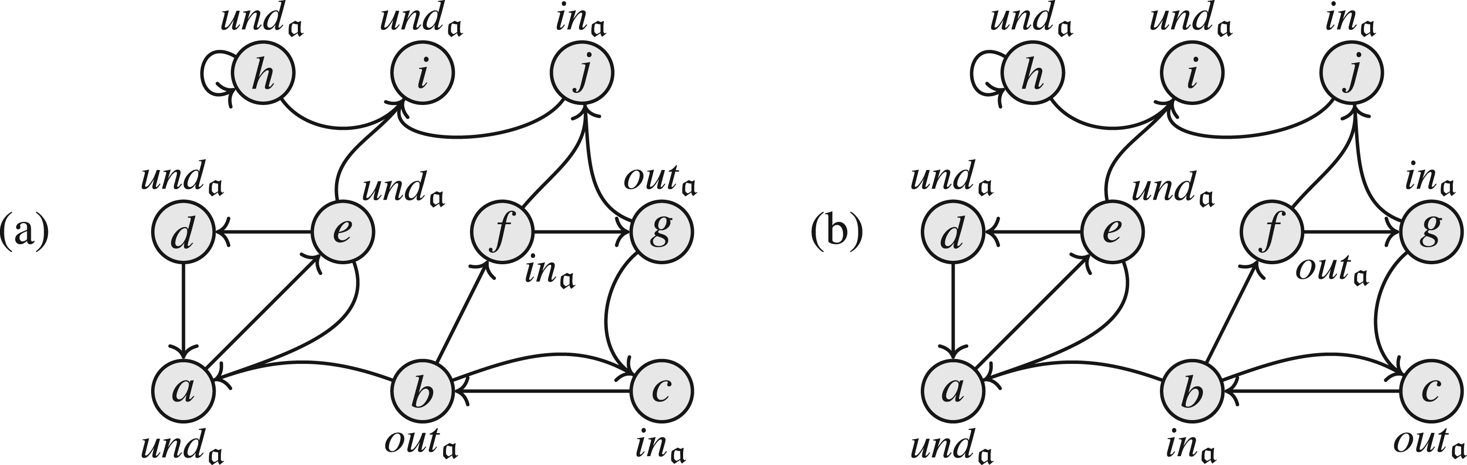
Speedup for stable semantics
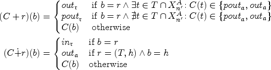
If our goal is to compute the stable extensions or reason in stable semantics, we can in fact apply a shortcut to the computation. Algorithm 2 depicts the steps we perform to compute the stable extensions given a backdoor set B. Since for a stable extension E each argument is either in E or attacked by E, we do not need to compute undecided arguments. While we still need to call a function to detect conflicts or undefended arguments, we can stop as soon as we have to assign the label for the first time. For this reason, we can use the updated function which we define as follows:
Consider the following propagation rules for :
set if and there is s.t. ,
set if and there is no s.t. .
We define as the result of initializing with on , and if rule (3) or (4) is applicable to any argument, we apply the rule once and return the resulting labeling.
One can see that this function in Definition 17 differs from the of Definition 10 only in that the application of rules (3) and (4) happens at most once.
Let be a SETAF class, let be a SETAF, and a backdoor for with . With Algorithm 2, we can enumerate all extensions in time .
Effectively, Algorithm 2 will compute all sets that Algorithm 1 also computes that contain no undecided arguments. While the asymptotic runtime of this improved version is still , we obtain a speedup for the function (the runtime of which is hidden in the term ).
Enumerating complete extensions
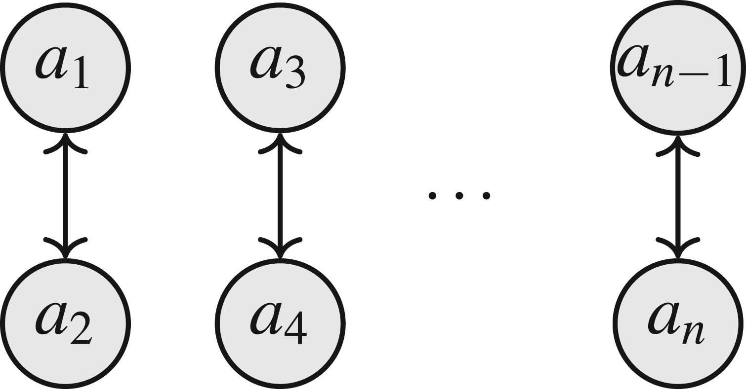
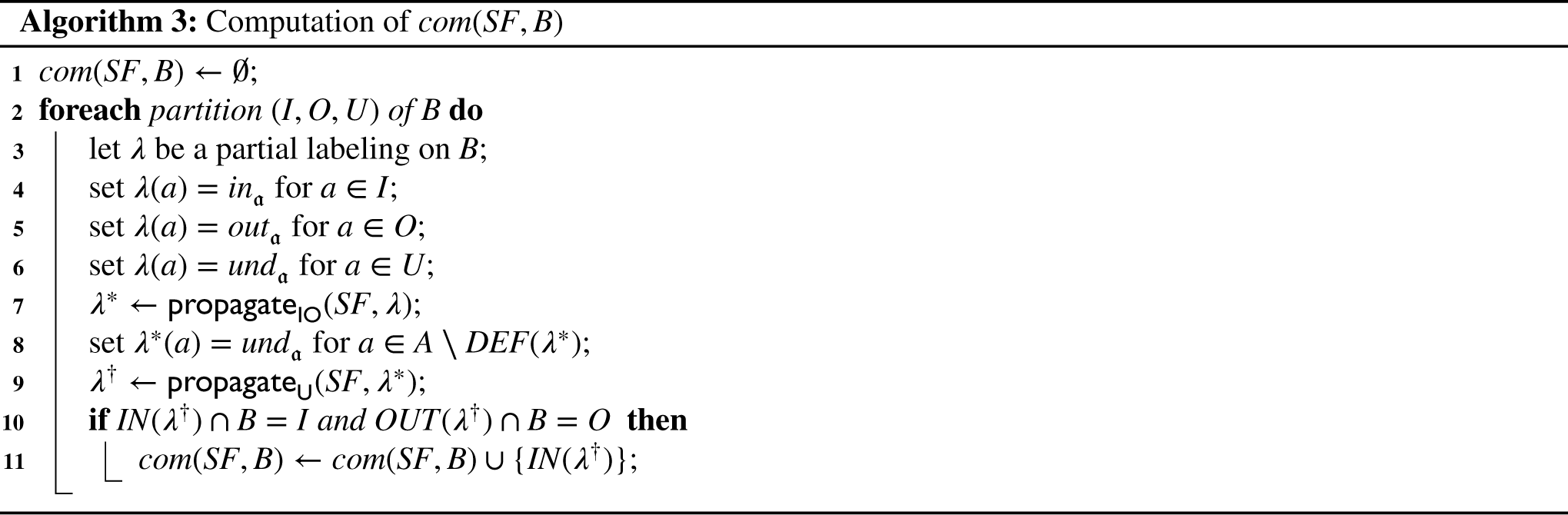
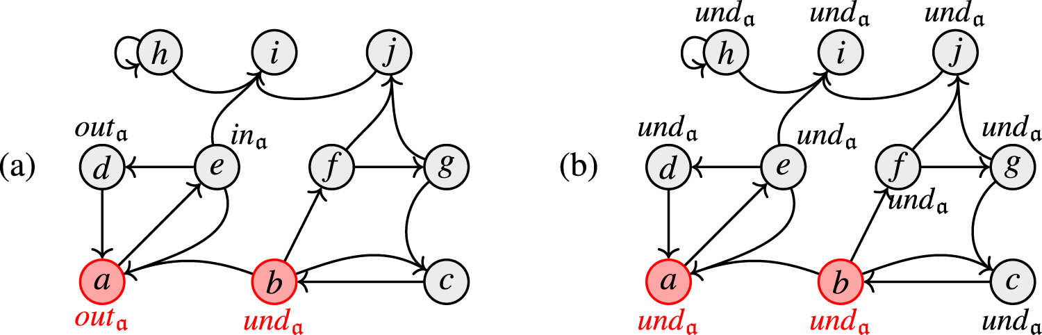
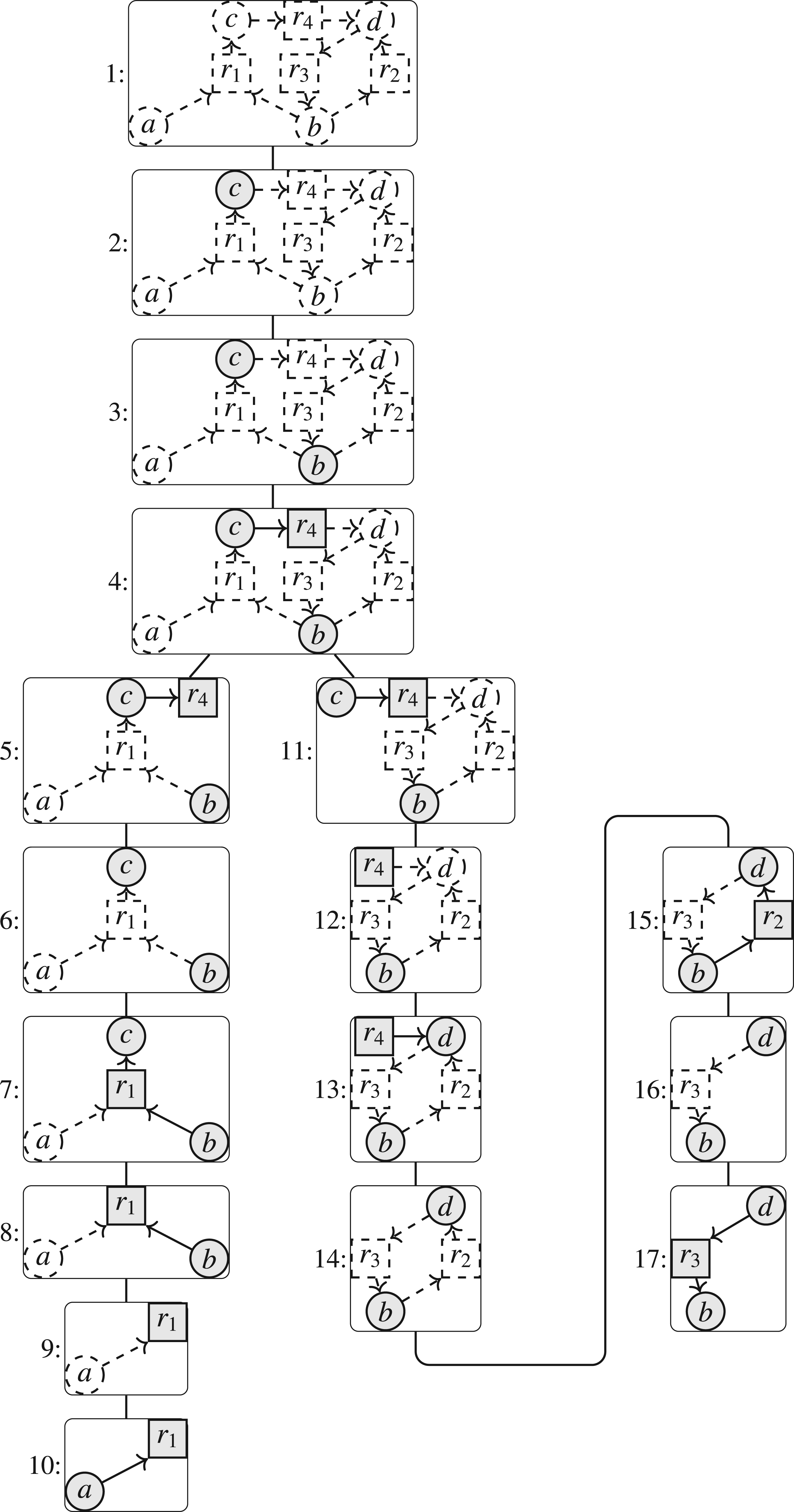
In the following, we present an algorithm to enumerate the complete extensions of a SETAF. Note that we cannot hope to enumerate the complete extensions in time w.r.t. the or backdoor of size p, as the example in Figure 5 illustrates: while the smallest backdoor is of size , there are complete extensions. Intuitively, this is due to the fact that in contrast to preferred extensions, in a “choice” like the even-length cycles in Figure 5 complete extensions have the three possible outcomes for arguments that correspond to the argument being in, out, or undecided. Crucially, the arguments can be undecided even though via the efficient backdoor algorithm for preferred extensions it would be possible to find supersets of admissible arguments. Hence, we generalize the “standard” backdoor evaluation approach of AFs by Dvořák et al.15 with a three-valued guess on the backdoor arguments. The revised Algorithm 3 contains the same basic steps as the algorithm for preferred extensions. This means we can use similar strategies to show the correctness and completeness of the algorithm. To this end, we use to compute the complete extensions of a SETAF via backdoor B.
SETAF with n arguments and a minimal backdoor of size . For each of the p pairs of mutually attacking arguments a complete extension can contain either or or neither of the two, resulting in complete extensions.
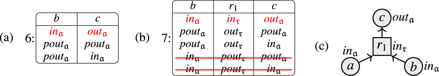
Again, we show that the two propagation algorithms and perform as expected. First, for the application of note that no label will be propagated (these labels will effectively be ignored). The only effect of these labels is “blocking” the application of a propagation rule that would “fire” in the algorithm for preferred semantics: in the example from Figure 5 if is a backdoor argument and is set to , the argument is labeled as via . If, on the other hand, we set to , no label will be assigned to via the exhaustive application of . An example of the execution of Algorithm 3 is shown in Figure 6.
Example for the backdoor algorithm for complete extensions. The backdoor and the guessed partition on B are highlighted. (a) Shows the outcome of the application of , (b) shows the outcome of the application of and the characterized complete extension .
Let be a SETAF, let , and a NOEVEN backdoor for . For the input to Algorithm 3, assume in step 2 we choose , , and . Let be the corresponding partial labeling from steps 4, 5 and 6. Set . Then for each :
if then ,
if then ,
if then ,
, and
.
Note that after step 8 the only arguments with an label are the ones in B we initially labeled this way due to our three-valued guess. In step 9, we apply the label to the remaining (unlabeled) arguments and again fix the mislabeled arguments.
Let be a SETAF, let , and a NOEVEN backdoor for . For the input to Algorithm 3, assume in step 2 we choose , , and . Let be the corresponding propagated partial labeling from step 8 with labels. Set . Then .
Finally, combining Lemmas 19 and 20, we obtain similar to Theorem 14 the following enumeration result for complete extensions. The final check-in step 11 ensures that we only keep the complete extensions that correspond to the initially guessed partition of B. Note that due to the three-valued guess, we obtain the factor .
Let be a SETAF class, let be a SETAF, and a backdoor for with . With Algorithm 3, we can enumerate all extensions in time on input .
Conditional lower bounds for backdoor evaluation
In this section, we show a so-called conditional lower bound29 for backdoor evaluation, that is, we show that our algorithm is basically optimal based on some well-known conjecture. The conjecture we are going to use is the strong exponential-time hypothesis (SETH).30,31 We show this for AFs; the result carries over to SETAFs.
SETH
For each there is a k such that k-CNF-SAT on n variables and clauses cannot be solved in time.
Let p be the parameter for the backdoor size. We will show that any backdoor evaluation that runs in time for AFs would violate SETH and thus imply a major breakthrough in the development of SAT algorithms.
Let be an AF and let and let p be the size of the given backdoor. There is no C-backdoor evaluation algorithm for for unless SETH is false.
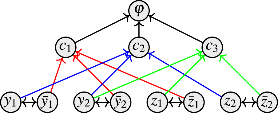
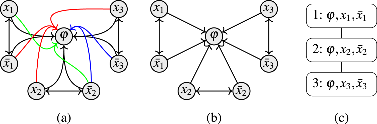
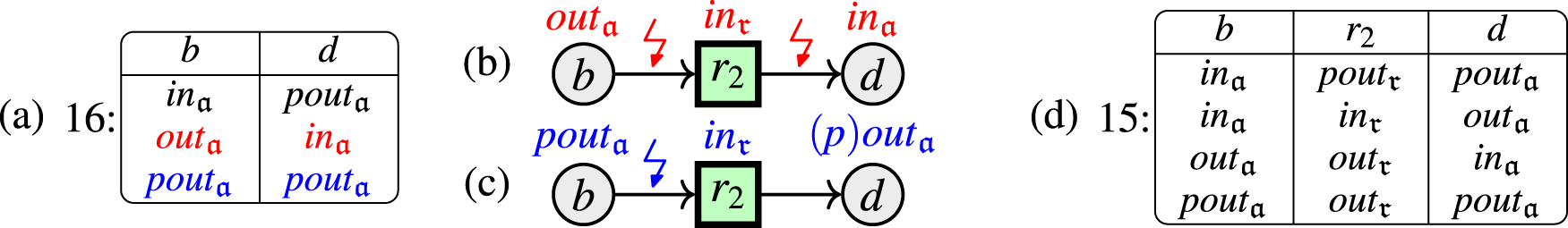
Given an instance from SETH, that is, a CNF formula with n variables and clauses. Let be the set of variables and be the set of clauses appearing in . Consider the standard translation24 from a CNF formula to an AF (cf. Figure 7) with and . We know that the formula is satisfiable iff the argument is credulously accepted w.r.t. .24 Moreover, we have that the set X is a C-backdoor of and has size n.
Illustration of the standard translation for .
Toward a contradiction let us assume we have a C-backdoor evaluation algorithm. Then we can decide whether a CNF formula is satisfiable as follows: We first construct the AF (which is polynomial in ) and then run the C-backdoor evaluation with backdoor X and return the answer for the credulous decision problem as an answer to the satisfiability problem. By assumption, the latter step has a running time of . That is, we have a algorithm for k-CNF-SAT for arbitrary , which contradicts SETH.
Treewidth-based algorithms
In this section, we discuss approaches to apply the notion of treewidth32 to SETAFs. Intuitively, the treewidth of a graph measures the “tree-likeness” of a graph. Since most reasoning problems remain tractable on trees, we can exploit this structure to construct efficient algorithms—given the graph is sufficiently “tree-like,” that is, has a low treewidth. On AFs, it has been shown that treewidth is indeed a parameter that allows for algorithms for reasoning,16 that is, the runtime is exponential only in the parameter value, but polynomial in the size of the framework. We will show that these results carry over to SETAFs, when we apply treewidth to the “right” underlying graph that adequately captures the intricate structure of SETAFs. The following concepts are illustrated in Figure 8.
Different graph and treewidth notions: (a) SETAF ; (b) incidence graph ; (c) primal graph ; (d) a tree decomposition of the primal graph; (e) a tree decomposition of the incidence graph.
Treewidth
Let be an undirected graph. A tree decomposition (TD) of is a pair , where is a tree and is a set of bags (a bag is a subset of ) s.t.
;
for each , the subgraph induced by in is connected; and
for each , for some .
The width of a TD is , the treewidth of is the minimum width of all TDs for .
In other words, a tree decomposition captures the structure of a given graph by constructing a tree . To each node we assign a bag containing vertices of the original graph s.t.
all original vertices are in at least one bag;
whenever a vertex appears in two bags and , the corresponding nodes are connected in via such that all nodes in between also have in their corresponding bags; and
for each edge of the original graph, for at least one node its corresponding bag contains both and .
As the treewidth is the smallest size of the largest bag minus 1 over all possible tree decompositions, trivially each graph has treewidth of at most (since it is always possible to put all vertices in a single bag of a tree decomposition). However, the lower the treewidth, the more tree-like a graph is by this measure. In particular, for trees, we obtain a treewidth of 1.
For fixed k it can be decided in linear time whether a graph has treewidth at most k; moreover, an according tree decomposition can be computed in linear time.33 For practical applications there are heuristic approaches available that will return decompositions of reasonable width very efficiently.34 However, as the underlying structure of SETAFs is a directed hypergraph, this notion is not directly applicable in our context. We can use “standard” directed graphs to describe SETAFs and apply treewidth by simply ignoring the direction of the involved arcs. For SETAFs there is the primal graph and the incidence graph as such notions, each of which leads to its own treewidth notion for SETAFs. First, we utilize the primal graph to define primal treewidth (recall Definition 5).
Primal treewidth
Let be a SETAF and its primal graph. The primal treewidth is defined as the treewidth of .
As mentioned earlier, several SETAFs can map to the same primal graph. However, restrictions on the primal graph are often useful to obtain computational speedups for otherwise hard problems.7,23 In contrast, the incidence graph uniquely describes a SETAF, as attacks are explicitly modeled in this notion. Note that the size of the incidence graph is linear in the size of the corresponding SETAF. Again, we utilize the incidence graph to define incidence treewidth.
Incidence graph
Let be a SETAF and let . We define the bipartite incidence graph of as with and . The incidence treewidth is defined as the treewidth of .
Figure 8 illustrates the ideas of Definitions 23 to 25. (a) Shows the SETAF , note that the attacks are named, (b) its primal graph, where we want to highlight how the collective attack is “split up” into the two edges and , (c) its bipartite incidence graph, with arguments on the left side and attacks on the right. In (d), we provide an example of a tree decomposition for the primal graph of . Clearly, is not a tree, which means the treewidth is at least 2. Since the tree decomposition in (d) has width 2 we can conclude that indeed . (e) Illustrates a tree decomposition of the incidence graph of . As before, we conclude .
We want to highlight that (a) both of these notions properly generalize the classical notion of treewidth commonly applied to Dung-style AFs and (b) these measures coincide on AFs. Formally:
The “standard” treewidth of AFs coincides with and .
The case of primal treewidth is immediate, as . For incidence treewidth note that we can construct from by substituting each edge by a fresh vertex and two edges , . It is well known that this operation preserves treewidth.
We will first show that reasoning on SETAFs with fixed primal treewidth remains hard (Section 6.1). Incidence treewidth on the other hand admits algorithms—we will initially establish this by characterizing the SETAF semantics via Monadic second-order logic (MSO)4,17 (Section 6.2). We utilize this characterization to obtain the desired upper bounds, as in this context we can apply a meta-theorem due to Courcelle.35,36 In a nutshell, it states that every graph property that can be characterized in MSO can be checked in polynomial time. However, this generic method typically produces infeasible constants in practice, which is why in Section 7 we will refine these results and provide a prototypical algorithm with feasible constants for stable semantics, later we refine our methods for admissible sets and complete extensions (cf. Dvořák et al.16).
Decomposing the primal graph
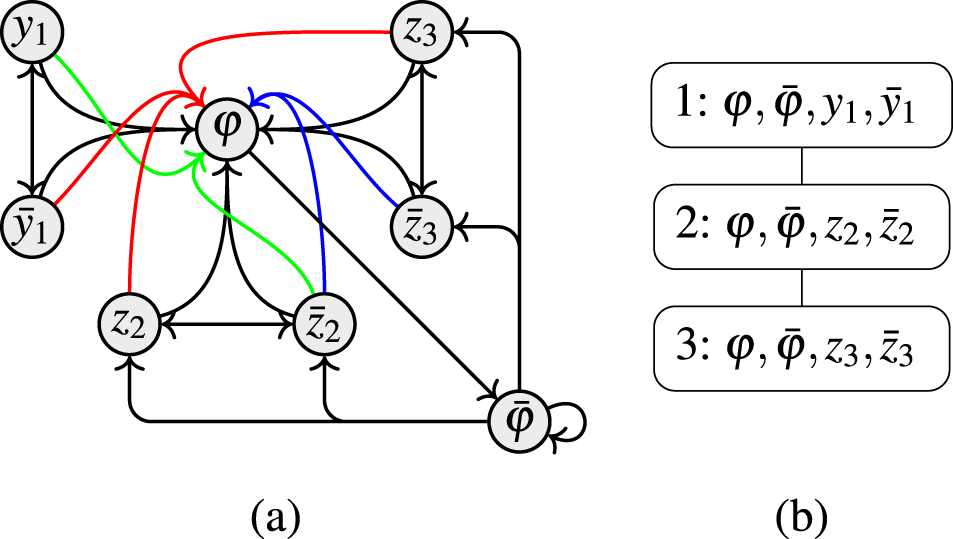
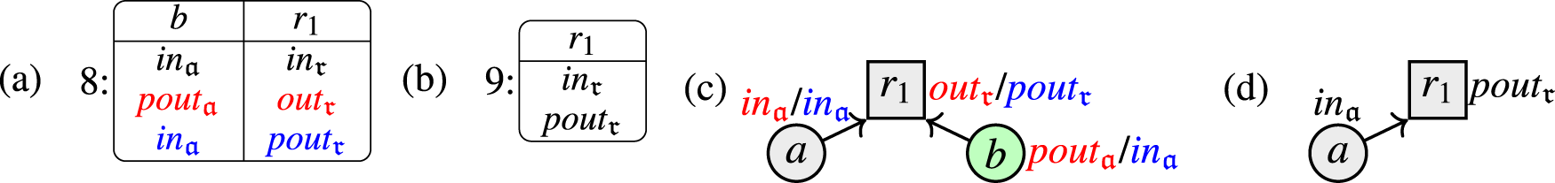
We start with an investigation of the treewidth of the primal graph. It has been shown that various restrictions on the primal graph can lead to computational ease.7,23 However, we will see that reasoning remains hard for SETAFs with constant primal treewidth (in contrast to the AF case, where we observe results). We establish this via reductions from (QBF-)SAT, illustrated in Figures 9 and 10. Intuitively, the attacks between the dual literals and represent the choice between assigning to true or false. The collective attack ensures that we take at least one of and into any extension in order to defend , making sure we only construct proper truth assignments. Finally, the remaining attacks toward correspond to the clauses and make sure that we cannot defend if for any clause we set all duals of its literals true—as this means the clause is not satisfied.
(a) The framework from the proof of Theorem 28 for , (b) , and (c) a tree decomposition of of width 2.
(a) from the proof of Theorem 29 for , and (b) a tree decomposition of of width 3.
The problems for are complete, and is complete for SETAFs with .
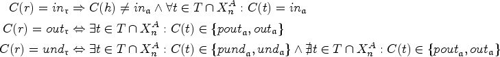
The membership coincides with the general case. For the respective hardness results, consider the following reduction from SAT (see Figure 9). Let X be the set of atoms and C be the set of clauses of a Boolean formula (given in CNF). We denote a clause as the set of literals in the clause, for example, the clause correspond to the set of literals (arguments, respectively) . By we denote the dual of a literal (e.g. and ). Let , where , and
Now it holds that is in at least one extension for if and only if is satisfiable.
() An admissible set E containing contains exactly one of each pair , as otherwise would not be defended against the attack . Moreover, as for each attack — consists of the duals of the literals in —this means at least one argument corresponding to a literal of each clause is in E. Hence, E corresponds to a satisfying assignment of .
() Every satisfying assignment of corresponds to a stable extension of : let be the interpretation satisfying , the corresponding set is then stable (admissible, complete, and preferred): As satisfies , for each attack corresponding to a clause not all tail arguments are in E, and hence is defended.
For the completeness result, we add an argument and an attack . If is unsatisfiable, will be attacked and will be contained in every stable extension. The constant primal treewidth is immediate, as illustrated in the example of Figure 9(c).
Also, preferred semantics reasoning remains intractable for SETAFs with fixed primal treewidth. For this result, we extend the construction from Theorem 28 by an additional argument that attacks the existentially quantified variables (see Figure 10).
is -complete for SETAFs with .
We show this by a reduction from the -complete problem. Let be a formula with in CNF. We construct the SETAF by extending from Theorem 28 in the following way (for an example see Figure 10): First, we set and add all arguments and attacks according to the construction of . Moreover, we add an argument and attacks . The last step is to add attacks for each . Now is in every preferred extension of if and only if is valid. We start with some general observations: cannot be in any admissible set, and can only be in an admissible set S if for each exactly one of and is in S. Moreover, in order to have , the argument has to be attacked by S, and consequently . This means for every admissible set S that corresponds to a satisfying assignment of the formula . In summary, every assignment on the variables corresponds to an admissible set, and every other admissible set in contains and represents a satisfying assignment for .
() Assume is in every preferred extension. Since every set is admissible and in order to accept for each either or have to be accepted, we know that for every assignment of variables there is an assignment satisfying .
() Now assume is valid, that is, for each assignment on the variables , there is an assignment on such that satisfies . From this and our observations above it follows that is in every preferred extension.
It is easy to see that the primal treewidth of is bounded by 3 (see Figure 10(b)).
Hence, under standard complexity-theoretical assumptions, these problems do not become tractable when parameterized by the primal treewidth.
Parameterized tractability via incidence treewidth
In this section, we establish tractability for reasoning in SETAFs with constant incidence treewidth by utilizing a meta-theorem due to Courcelle.35,36 In particular, we use the tools of MSO to characterize the semantics of SETAFs (similarly, this has been done for AFs4,17). MSO generalizes first-order logic in the sense that it is also allowed to quantify over sets. Domain elements in our settings are vertices of an (incidence) graph, that is, arguments or attacks. MSO in our context consists of variables corresponding to domain elements (indicated by lowercase letters), and set variables corresponding to sets of domain elements (indicated by uppercase letters). Moreover, we use the standard logical connectives , as well as quantifiers for both types of variables. Hence, given a graph , an MSO formula depends on open variables in the form of vertices , and sets of vertices (while we could also have open variables in the form of edges and sets of edges, we do not make use of this in the following characterizations). We recall Courcelle’s theorem in the style of Dvořák et al.17
For every fixed MSO formula and fixed integer there is a linear-time algorithm that, given a graph of treewidth , decides whether given , , satisfy .
We use the unary predicates and to indicate an element being an argument or an attack of our SETAF, respectively. Moreover, we use the binary predicate to indicate an edge in the incidence graph between incidence vertices and . Alternatively, we write , , for , respectively. Based on these basic definitions, we define notational shortcuts to conveniently characterize SETAF properties. Let be a SETAF and its incidence graph. We define the following notion for and : let be shorthand notation for . This notion consists of four parts: (1) vertex corresponds to an attack, (2) h is the head of the attack , (3) the arguments in T constitute the tail of . We utilize this to avoid dealing with the attack vertices of the incidence graph in our semantics characterizations. We borrow the following “building blocks” from Dvořák et al.17 (slightly adapted for our setting).
We can express (subset)-maximality and -minimality for any expressible property as follows17:
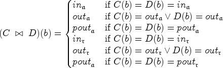
Having these tools at hand, we can characterize the SETAF semantics in an intuitive way. It is easy to verify that these exactly correspond to the respective notions from Definition 4. Utilizing these building blocks, we can encode the semantics exactly as in AFs.4,17
Let be a SETAF and let be its incidence graph. For a set where :
Reasoning and verification can then be done in an intuitive way, see Dvořák et al.17 For example, to find out whether an argument a is credulously accepted w.r.t. stable semantics we can use the formula . We can immediately apply Courcelle’s theorem35,36 to obtain the desired result.
Let be a SETAF. For the semantics under our consideration, reasoning is fixed-parameter tractable w.r.t. the incidence treewidth .
Dynamic programming on SETAFs
In the following, we specify three dynamic programming algorithms utilizing incidence treewidth to reason in stable, admissible, and complete semantics. Ultimately, we will show that these algorithms allow us to reason efficiently in SETAFs with fixed incidence treewidth. Note that we put some of the proofs in Appendix B to improve the readability of the paper.
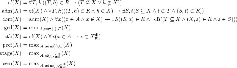
As an overview, we illustrate the key steps in the dynamic programming approach for treewidth in Figure 11. The first step is to compute the incidence graph, then we obtain a tree decomposition for the incidence graph. For each node of the tree decomposition, we can compute the extension candidates for the corresponding subproblem. This is done in a bottom-up manner, that is, a root node for the tree decomposition is chosen, and this node will be computed last. Starting from the leaf nodes, we compute the subsolutions (depending on the node types as we will discuss next) for each node where all child nodes are done. Note that this can also be done in parallel. Finally, once the root node is computed, the solution candidates exactly characterize all extensions, and reasoning, counting, and enumerating can be performed with this implicit representation of the extensions. In the following, we introduce the details of this process.
Overview of the dynamic programming approach.
To illustrate the underlying idea of all three of these algorithms, we restrict the tree decompositions of the incidence graph to nice tree decompositions.
A tree decomposition is called nice if is a rooted tree with an empty bag in the root node, and each node (shorthand notion for ) is of one of the following types:
Leaf: n has no children in .
Forget: n has one child , and for some .
Insert: n has one child , and for some .
Join: n has two children , , with .
Any tree decomposition can be transformed into a nice tree decomposition with the same width in linear time.37 Let be a SETAF and . For sets , by , we identify the sets , , respectively. By we denote the union of all bags where appears in the subtree of rooted in n. Likewise, by we denote the set .
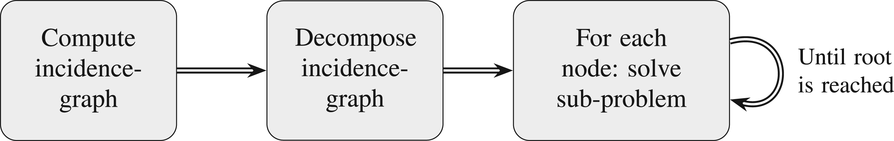
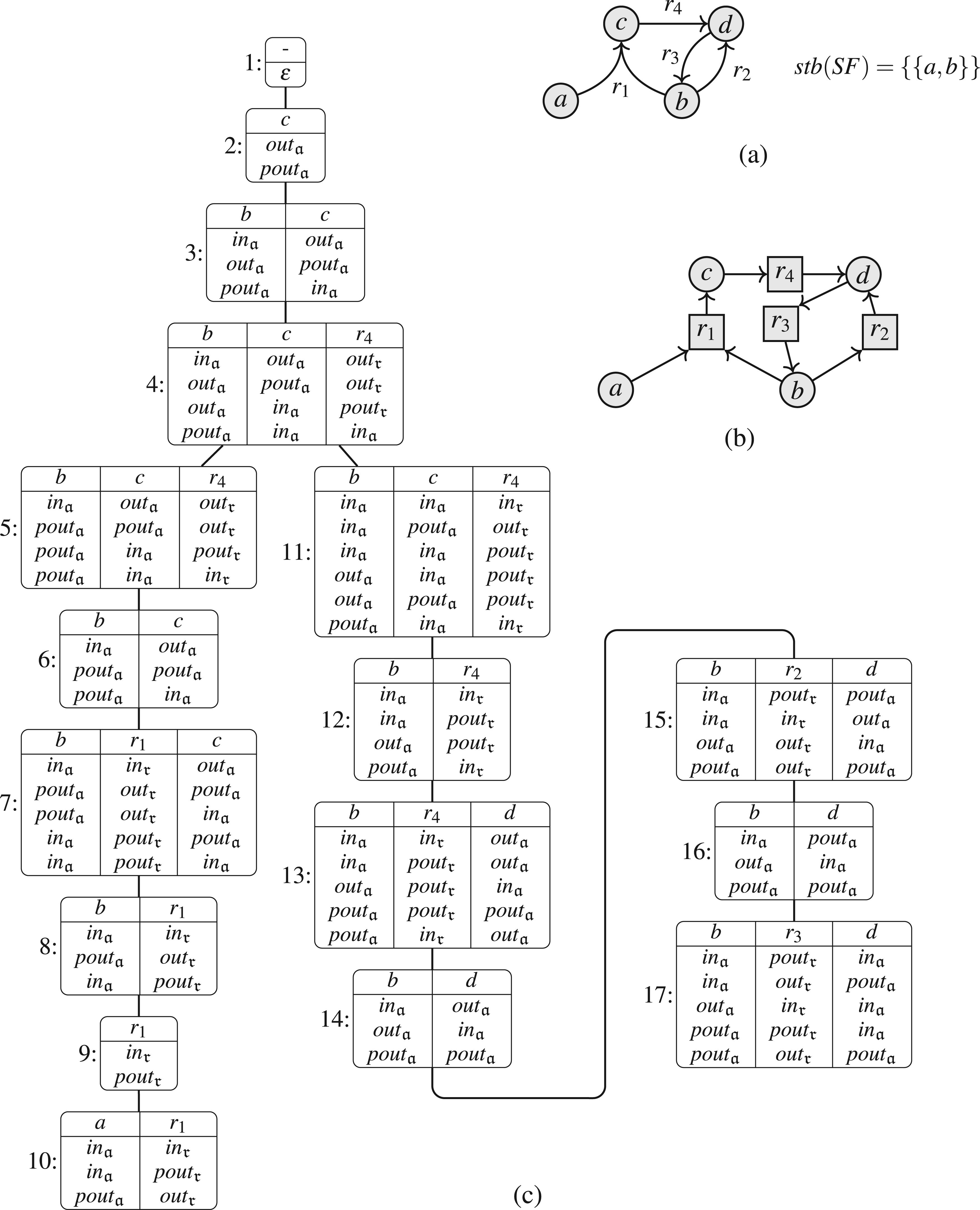
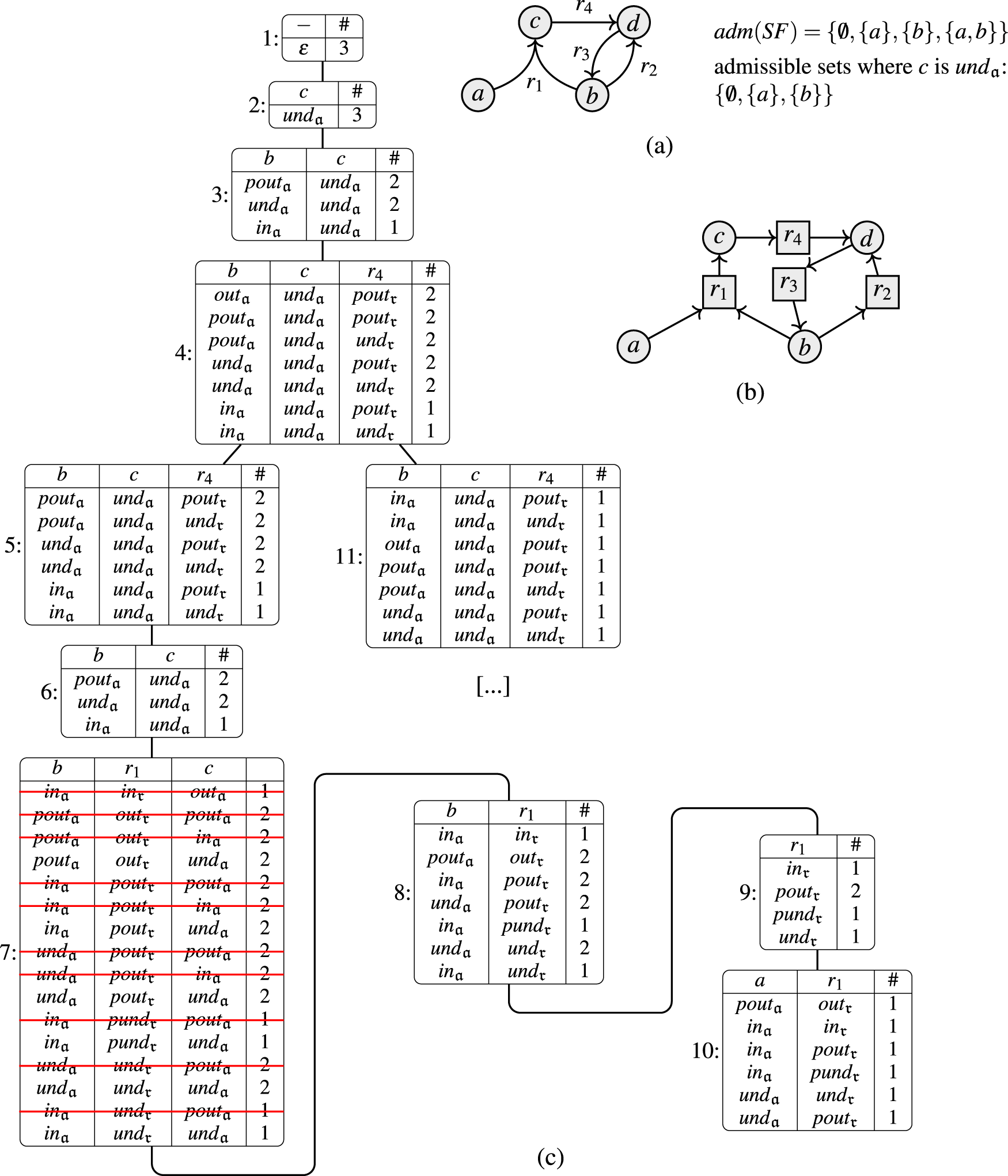
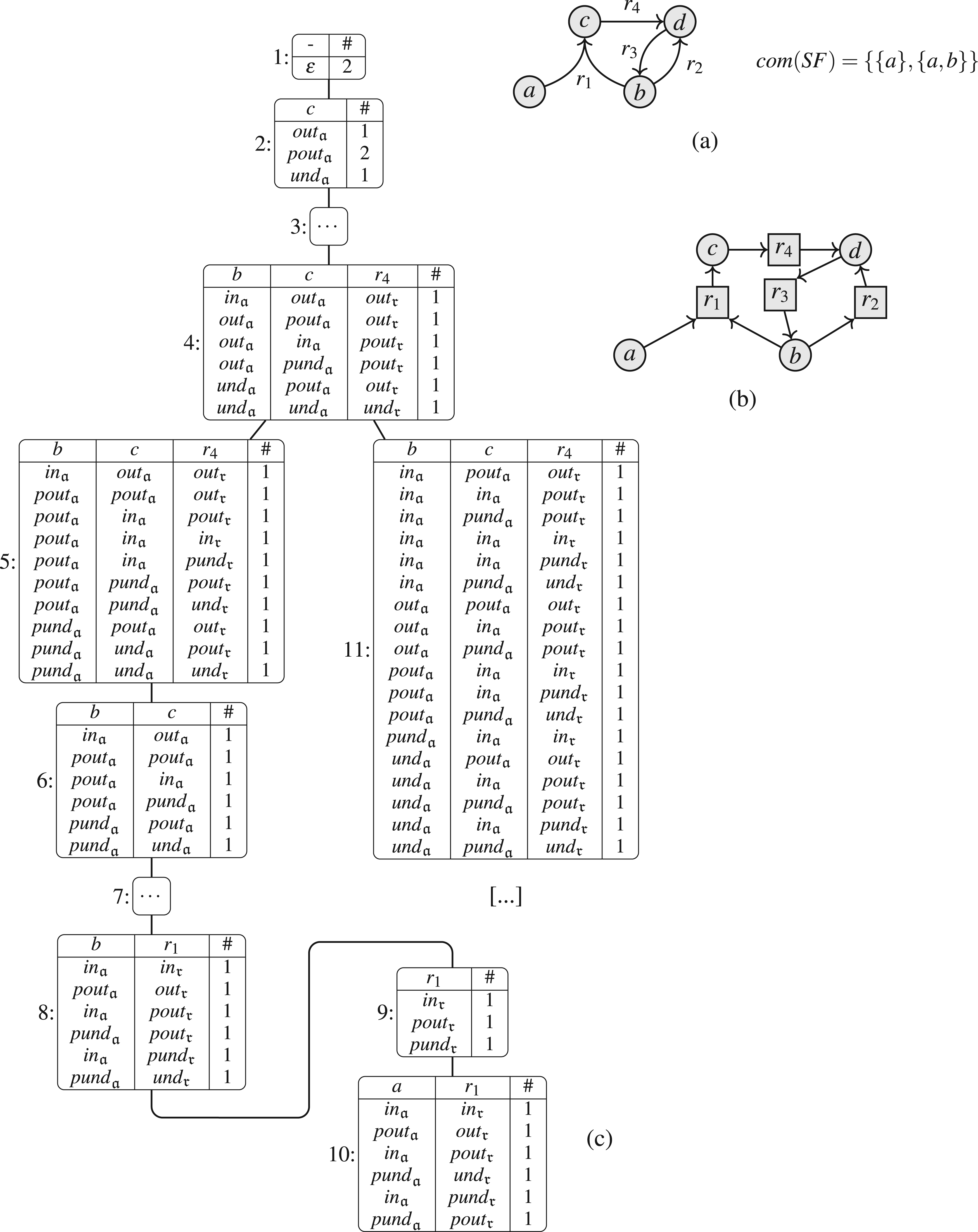
We exemplify the notation with our running example, illustrated in Figure 12. If we focus on node 5, we have , with , and . The subtree rooted in node 5 contains the nodes 5–10. Consequently, we have and . We illustrate the relevant parts of the SETAF for each node in Figure 13.
Running example for Section 7: (a) SETAF ; (b) incidence graph ; (c) nice tree decomposition of .
Running example ctd.: for each node, we illustrate the parts of the SETAF rooted in the subtree (dashed + non-dashed) and the arguments/attacks of the current node (non-dashed).
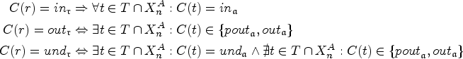
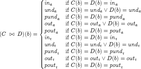
We use colors to keep track of the arguments and attacks that appear in the bag of node . We call an assignment of colors to arguments and attacks a coloring—they are akin to the idea of labelings for SETAFs, which is an alternative though (mostly) equivalent approach for SETAF semantics.25 However, note that in our case we also color (or “label”) the attacks in addition to the arguments, similar in spirit to attacks semantics.26,38 In our case, these colorings characterize extension candidates w.r.t. nodes in the tree decomposition that are consistent with the subframework rooted in the node in question. Consequently, as the framework rooted in the root node of the decomposition is the entire framework, the colorings in the root node characterize the extensions of the SETAF. Let be a SETAF. For an argument , we use different colors to indicate its relation to an extension . The color indicates (a is “accepted”), indicate (a is “defeated”), and indicate (a is “undecided”). We use two colors each for defeated and undecided arguments, respectively, to ensure the correctness of our algorithm. The colors and correspond are in a sense “provisional” in that the “responsible” attack has not yet appeared in the bottom-up computation along the tree decomposition. Likewise, for attacks we use the colors if all are ; if one is or ; for the case where we expect at a later stage in the algorithm to add some that is or ; if one is or (and no is or ’); and for the case where we expect at a later stage in the algorithm to add some that is or (and again no is or ’). Note that the exact interpretation of the colorings will be discussed in detail when we investigate each semantics, as we will be able to optimize the colorings tailored to each semantics. For example, we do not need to consider undecided arguments or attacks in stable semantics, as no extension can contain these.
Characterizing stable extensions
In the following, we give a detailed account of how to characterize stable extensions via dynamic programming on the incidence-tree decomposition. In this regard, we define so-called st-colorings for each node of the tree decomposition in a way that can easily be implemented in a system. Moreover, we define stable colorings, that is, the desired colorings for each node. Ultimately, we show that st-colorings and stable colorings coincide and thereby show the correctness and completeness of our algorithm.
As in a stable extension E we only have arguments either in E or attacked by E, we do not need to consider the undecided colors. After all, no extension candidate with undecided arguments or attacks in it can be extended to a stable extension. Hence, the colors we use for the dynamic programming algorithm for stable semantics are given as follows:
In the following, we assume we are given an arbitrary but fixed SETAF , as well as a corresponding nice tree decomposition of .
We next characterize the stable colorings for each node of the tree decomposition. The stable colorings of a node characterize the candidates for stable extensions, as per the information that is available up to the current node. That means, in the root node (where information about the whole SETAF is available) the stable colorings correspond exactly to the stable extensions of the SETAF. We will later define st-colorings as the output of our algorithm and show that st-colorings and stable colorings coincide.
We relate a coloring of a specific node n to a (hypothetical, not actually computed) generally larger coloring on all the arguments and attacks of the subtree rooted in node n (i.e., on all elements in ). For the root node, this subtree contains all arguments and attacks of the SETAF, which ensures that the colorings in the root in fact correspond to the stable extensions, as we will show in Proposition 36.
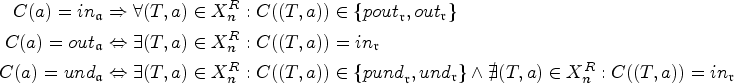
A coloring for a node is stable if we can extend C to a coloring such that the following conditions are met for each and each :
if then ,
if then ,
if then ,
if and only if ,
if then , and
if and only if .
For a coloring C in node n we define by the set of such extended colorings on s.t. (1) to (6) are met. These are the characterized colorings.
We now give some intuition for this definition. For the extended coloring we require six conditions (1) to (6) to be satisfied. (1) and (2) ensure that for all the arguments/attacks that only appear below a current node (i.e., in the subtree rooted in the node, excluding the node itself) only non-provisional colors are used. This is because, by the properties of tree decompositions, we will not “encounter” these arguments/attacks again in the remaining computation; hence, provisional colors could not be “confirmed” to become non-provisional, and could therefore never be extended to an actual stable extension of the SETAF. (3) and (4) capture the requirements of stable extensions for arguments, that is, if an argument is in then all attacks toward the argument must be out, and if an argument is out then at least one attack toward it must be in. Note that these conditions effectively characterize admissibility, but since we only allow two options and for arguments and every argument has to be colored, this suffices to characterize stable extensions. Similarly, (5) ensures that for each attack that is in all of the arguments in the tail of the attack are in, and (6) makes sure that for each attack that is out at least one tail argument is out. These last two requirements make sure that the colors of the attacks correspond to the desired intuition, namely: (5) an attack is colored if and only if it is “effective,” that is, all of its tail arguments are in the characterized stable extensions and the head of the attack is indeed attacked, and (6) an attack is colored or if at least one of the tail arguments is attacked by the characterized extensions E which renders the attack “ineffective” and h is defended against the attack (by whatever attack is responsible for attacking ).
We now illustrate the purpose of the colorings, namely that the characterized colorings of the root node correspond to the stable extensions of the SETAF.
Let be a nice tree decomposition of a SETAF and let be the root node of . Moreover, let be the set of stable colorings for . Then
Since the root node is empty, we have that and , which by (1) and (2) means that we have no provisional colors in each extended coloring (in case there is a stable coloring , that is, ). Finally, conditions (3) and (6) give us the following property (a) and (4) and (5) give us the following property (b):
If then , and
if and only if .
(a) Exactly characterizes conflict-freeness, that is, for each attack toward an argument a that is in the extensions (i.e., in the set ) there is at least one argument in T that is not in the extension. (b) Characterizes the fact that every argument that is not in the extension is attacked by the extension (since for stable semantics the only options for arguments are the colors and ). (a) and (b) together exactly define the stable extensions.
We want to point out that since the root node of a nice tree decomposition is always empty, we have either or , that is, either there are no colorings in or the empty coloring . In the first case, Proposition 36 tells us that there are no stable extensions; in the second case the characterized extended colorings characterize the stable extensions. Intuitively, the actual extensions can be computed by straight-forwardly combining the corresponding colorings of one branch of , wherever a coloring “persists” throughout the whole branch. All extensions can be enumerated this way with linear delay (for details see Jakl et al.39).
We will now continue to discuss the four node types and show that in each node we indeed capture exactly the stable colorings. In particular, we present the algorithm itself (i.e., define the st-colorings), and show that we characterize all the stable extensions and only stable extensions (i.e., that each intermediate coloring in each node is stable as per Definition 35).
Leaf nodes
Intuitively, in leaf nodes for each argument and each attack, we guess one of two possibilities: or (in the second case we use either or , as we will explain below). We then keep every “consistent” coloring, for example, if an argument is colored then there cannot be an attack toward it that is colored . Whether (i) an argument or (ii) an attack is colored or depends only on whether the color is “confirmed,” that is, (i) for arguments whether there is an attack colored toward the argument, and (ii) for attacks whether there is an argument colored in the tail of the attack.
St-colorings: Leaf
An st-coloring for a leaf node is each coloring that satisfies the following conditions. For each argument :
For every attack :
In our running example in Figure 14, the nodes 10 and 17 are leaf nodes. Note that there is no explicit condition for the colors and . This reflects the fact that we can color any argument/attack provisionally out (as long as it does not violate any of the conditions for the other colors) which captures the situation where an argument is going to be attacked by an attack that we have not yet considered, that is, that is still going to be handled in a later (i.e., upper) node in the tree decomposition.
All st-colorings for our running example. (a) Our running example SETAF with its stable extensions, (b) its incidence graph , and (c) all st-colorings for w.r.t. the tree decomposition given in Figure 12.
For the following lemmas note that for leaves it holds . Then the following two results directly follow from Definition 35 of stable colorings and Definition 37 of st-colorings in leaves. The following lemma captures the soundness of our algorithm and holds because the conditions for st-colorings imply the properties of stable colorings.
Each st-coloring C for a leaf node is stable.
The next result captures the completeness of our algorithm and holds because the properties of stable colorings imply the conditions for st-colorings for leaves.
Each stable coloring C for a leaf node is an st-coloring.
Forget nodes
We examine forget argument nodes and forget attack nodes separately. Let n be a forget argument node with child such that . We have to discard all colorings C where , as in these colorings a is supposed to be attacked by the extensions that C potentially characterizes. However, as we forget a in the current node by the definition of a tree decomposition, this cannot happen: consider again the running example from Figure 14. Node 9 is a forget node, where the argument a is forgotten (we illustrate this situation in Figure 15). This means that in the “upper” part of the tree decomposition, no attacks toward a can be added. Hence, there cannot be an attack colored toward a that confirms a being attacked, and the provisional color cannot be updated to . One can clearly see that this behavior is correct, as there is indeed no attack toward a in .
St-coloring: Forget argument
Let n be a forget argument node with child such that , and let C be an st-coloring for . If , then is an st-coloring for n, where for each is defined as follows:
St-colorings for leaf nodes and forget argument nodes. Example for st-colorings for (a) the leaf node 10 from Figure 14 and (c) the “Forget a” node 9 for argument a. Subfigure (b) illustrates the subgraph of the incidence graph that corresponds to the leaf node together with the coloring that is discarded by the forget node.
We handle forget attack nodes in a similar way, that is, we discard colorings where the attack we forget is provisionally out. In this case, we colored the attack at an earlier stage in the algorithm, anticipating the possibility of an insert argument node where a tail argument is colored or . Due to the properties of the tree decompositions, such an insert argument node cannot appear above the forget attack node, which is why we can discard colorings where the attack is colored provisionally.
St-coloring: Forget attack
Let n be a forget attack node with child such that , and let C be an st-coloring for . If , then is an st-coloring for n, where for each is defined as follows:
Next, we show the soundness of our algorithm for forget nodes. This result carries over from the child node, as we discard colorings where the forgotten argument/attack is provisional. Let us revisit a part of our running example (see Figure 16), we see in node 6 (where we “forget” the attack ) that we “copy” each st-coloring of the child node 7 except for the last two colorings where has the provisional color (Figure 16(b)). It is then clear that since each st-coloring of node 7 can be extended to a coloring on all of (since we assume these colorings are stable) that the same holds for the st-colorings of node 6. For example, the st-coloring of node 7 with , , and can be extended to the coloring on with (and of course for ); analogously the st-coloring C of 6 with and can also be extended to on , and it can easily be checked that C is stable.
St-colorings forget attack nodes. Example of (a) the forget node 6 and (b) its child node 7 from the running example (the discarded colorings are struck out). (c) Illustrates the subframework rooted in 6 (i.e., containing ) and an extended coloring that extends the highlighted colorings of (a) and (b).
If for the child node of a forget node n each st-coloring is stable, then each coloring C of n is stable.
To show the completeness of our algorithm, we can show that for each stable coloring C for node n there has to be a corresponding st-coloring in the child node such that for the forgotten argument/attack . This means that n contains every stable coloring. The key idea is that in the child node coincides with C and does not color in a provisional color, as otherwise, C would not be a stable coloring for n. Again consider node the forget node 6 of our running example (Figure 16). Even without knowing that coloring C with and is a st-coloring of node 6, we can check that this coloring is stable for node 6. This means we can extend it to a coloring on , and we can infer that there has to be a stable coloring for the child node 7 that can also be extended to . As with the other direction, we then see that indeed .
Let C be a stable coloring of a forget node n. If in the child node of n stable colorings and st-colorings coincide then C is a st-coloring for n.
Insert nodes
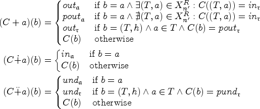
We distinguish the two cases where we insert an argument and insert an attack. Whenever we insert an argument a, we have to consider up to two different scenarios: : the added argument is attacked by the characterized extension. In this case, the added argument is colored or , depending on whether the “responsible” attack is already in the current bag. In case a is in the tail of an attack, we can color this attack . : the added argument is in the extension. In both cases, we have to check whether the result will be consistent with the existing colors, that is, for the added argument must not be in the tail of an attack that is colored , and for there must not be an attack colored toward the added argument. Assume we would color the inserted argument b as while b is in the tail of attack , which we already colored in a previous step. Of course, this is not consistent with our intended meaning of the attack color . On the other hand, assume we color b as while it is attacked by which we already colored in a previous step. This would introduce a conflict in the constructed extension.
St-coloring: Insert argument
Let n be an insert argument node with child such that , and let C be an st-coloring for .
If , then is an st-coloring for n.
If , then is an st-coloring for n.
The operations and are defined as follows for each :
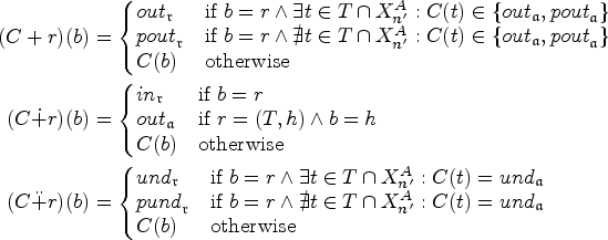
For insert attack nodes, we also have to consider two cases for an attack : : the extension attacks T, either in the current bag (in which case we color the attack ) or possibly in the “upper” parts of , then we color the attack . : this case indicates for the extension E. In this case, the head of the attack can be set to . Again, we can only apply this coloring if it is consistent with the previous colors. The idea is very similar to the insert argument nodes; we exemplify the issues in Figure 17: in (b), we cannot color the added attack with due to two issues, namely (1) the argument b in the tail of is not colored , and (2) the head of (argument d) is already colored . In (c), we cannot color with even though the head is matching, because the tail argument b is not colored . We will use the operations and as given in Definition 45.
St-coloring: Insert attack
Let n be an insert attack node with child such that , and let C be an st-coloring for , and .
is an st-coloring for n.
If , then is an st-coloring for n.
The operations and are defined as follows for each :
St-colorings for insert attack nodes. (a) Shows the st-colorings for node 16 and (d) the st-colorings for “Insert attack ” node 15 from Figure 14. Subfigures (b) and (c) show inconsistent colorings.
Again, we show that the insert nodes exactly characterize the stable colorings. For the following lemma (soundness), we need to show that each of the colorings of an insert node n is stable. It can be shown that in both cases, that is, when the st-coloring C in node n is constructed either from an st-coloring of child node via or (for an argument/attack ) all conditions (1) to (6) of stable colorings hold. This is ensured either via the requirements for adding or or by construction by the assigned colors. In particular, the colors and are assigned according to whether the “confirming” argument/attack is already present in the current node n. This together with the fact that the original st-coloring of the child node is stable—the basis for the constructed coloring C in n—ensures that C is stable as well. For example, consider in our running example the insert node 8 (illustrated in Figure 18). Its child node 9 contains an st-coloring with . For 8, we get and (Figure 18(a)). In , we set , which “confirms” the provisional color of and “upgrades” it to , the corresponding extended coloring on is illustrated in Figure 18(c). In , on the other hand, we set and keep , the corresponding extended coloring is also illustrated in Figure 18(c). Since we update the color of only because we have “proof” to do so, we can check that these st-colorings are stable.
St-colorings for insert argument nodes. Example of (a) the insert node 8 with highlighted colorings (red) and (blue), and (b) its child node 9 from the running example. (c) Illustrates the subframework rooted in 8 (i.e., containing ) and extended colorings (red) and (blue), (d) illustrates the subframework rooted in 9 with the extended coloring .
If for the child node of an insert node n each st-coloring is stable, then each st-coloring C of n is stable.
For the following result (completeness) we can show that for each stable coloring C in the insert node n there has to be a corresponding st-coloring in the child node on all of such that or for the added argument/attack . The key idea here is that differs from C exactly in those cases where the added argument/attack leads to non-provisional colors in C, these colors we set to in . We can then check that all conditions of stable colorings are satisfied for , and since we assume that in the child node stable colorings and st-colorings coincide, we know that is an st-coloring of . Finally, it is easy to see that in both cases the requirements for adding or as an st-coloring for n are satisfied. Revisiting the example of Figure 18, we can see that for both st-colorings and the corresponding st-coloring in node 9 has , which is due to the fact that there is no “confirming” argument in the tail of in . Since this coloring has to be a st-coloring of 9 and we can construct both and from , we can see that these two stable colorings are indeed st-colorings of node 8.
Let C be a stable coloring for an insert node n. If in the child node of n stable colorings and st-colorings coincide then C is a st-coloring for n.
Join nodes
In these nodes, we combine the colorings of immediate child nodes. The colored arguments and the colored attacks of the (to be) combined colorings have to coincide to yield an st-coloring for the join node. Whenever at least one of the child node colorings has a non-provisional color (on arguments or attacks), the non-provisional color carries over to the resulting coloring in the join node. This is because it means in at least one of the sub-trees the color has been “confirmed.”
St-coloring: Join
Let n be a join node with children , let C be an st-coloring for , and let be an st-coloring for . If and then is an st-coloring for n, where
Again we show that our algorithm for st-colorings is correct, that is, that the conditions (1) to (6) of Definition 35 are satisfied. Since we assume that the colorings C and in the child nodes and are stable, the conditions for the join node n are satisfied by : the subframeworks rooted in nodes and are parts of the subframework rooted in n which means all conditions carry over. This situation is illustrated in Figure 19. Note how in Figure 19(a) the provisional color for b of C (Figure 19(b)) and for of (Figure 19(c)) are “upgraded” to non-provisional colors and , respectively. This is because b is colored in and is colored in C, which means for the join node 4 that the “proof” for the non-provisional colors occurs in the subframework.
St-colorings for join nodes. Example of (a) the join node 4 with highlighted coloring , (b) its child node 5 with highlighted coloring C, and (c) its child node with highlighted coloring .
If for the child nodes of a join node n each st-coloring is stable, then each st-coloring C of n is stable.
To show the other direction, that is, completeness of our algorithm for join nodes, we have to show that for each stable coloring C in join node n there are st-colorings and in the child nodes of n s.t. and therefore C is an st-coloring of the join node. If we assume that C is stable, we can easily construct such and for the child nodes—for the construction, we have to take into account that the nonprovisional colors of C might be provisional in or (but not both), then we can easily check that the thereby constructed colorings are stable for the child nodes. For example, we can check that the highlighted coloring C is stable for node 4 in the running example, illustrated in Figure 19. When constructing the corresponding coloring for child node 5 we see that there is no possible attack toward b that is colored and we have to set . Similarly, we set since we can extend to a coloring on such that no argument in the tail of the attack is colored or . and are stable for their respective nodes 5 and , and in fact, we see in Figure 19(b) and (c), respectively, that the constructed colorings are indeed st-colorings.
Let C be a stable coloring for a join node n. If in the child nodes , of n stable colorings and st-colorings coincide then C is an st-coloring for n.
Final steps for stable semantics
Toward characterizing the stable extensions via our st-colorings, we can now utilize the soundness and completeness results that we established for each node type. We obtain the following results that underpin the adequacy of the algorithm.
Let be a nice tree decomposition of a SETAF . Then in each node st-colorings and stable colorings coincide.
() Follows by structural induction over the tree decomposition structure with the leaves as a base (Lemma 38) and the forget, insert, and join nodes as steps (Lemmas 42, 46, and 49).
() First note that by () all st-colorings in each node are stable. Then the statement follows by structural induction over the tree decomposition structure with the leaves as a base (Lemma 39) and the forget, insert, and join nodes as steps (Lemmas 43, 47, and 50).
Effectively, we established that the root node indeed characterizes the stable extensions. We can decide / for an argument by flagging colorings that contain/do not contain a. In each node, we update the flag accordingly; the flag in the root node indicates credulous/skeptical acceptance. We can keep the count of extensions w.r.t. each coloring, and to enumerate the extensions once the dynamic programming algorithm is done we can traverse the tree top-down and output the extensions with linear delay (cf.16,39). Hence, we obtain the following upper bound for the problems of stable semantics.
With the presented algorithm, as well as counting the number of stable extensions can be done in time . Moreover, we can enumerate all stable extensions with linear delay.
The correctness of the algorithm (i.e., we account only for stable colorings in the root node) and the completeness of the algorithm (i.e., we account for all the stable colorings in the root node) is shown in Proposition 51. Then, from Proposition 36 we get that we exactly characterize .
We can assume the number of nodes to be bounded by and that we can find and access rows in linear time w.r.t. k. For each node, the number of (valid) colorings (i.e., rows in our tables of colorings) is bounded by . In leaf nodes, we can check the colorings in time for each of the possible colorings, resulting in . In forget nodes, we can check the conditions and compute eventually resulting colorings in time for each of the colorings of the child node, resulting in . In insert nodes, we can check the conditions and compute eventually resulting colorings in time for each of the colorings of the child node, resulting in . Finally, for join nodes we have to consider pairs. However, we only need to consider pairs if we assume the data structure to be properly sorted, for example, lexicographically by treating the colors as 0 and as 1. As each table has rows, sorting is in . Let C be a coloring such that arguments/attacks are colored as . There exist at most distinct colorings with . There are possibilities resulting from the choice of , resulting in join pairs. We can then compute in , resulting in for join nodes, dominating the runtime of the other node types. The resulting runtime for the algorithm is .
Characterizing admissible sets
For admissible sets, we have to account for arguments that are neither in an extension nor attacked by it. Hence, we extend the colorings we used to characterize stable extensions to reflect these “undecided” arguments. In addition to the colors for arguments and for attacks, we consider the color for arguments, and the two colors for attacks. Intuitively, with the color, we indicate arguments that are neither in an admissible set E nor attacked by E (this situation is not allowed in stable extensions). The color indicates attacks that in relation to an admissible set E neither attack E (i.e., have ) nor have a defeated argument in their tail (i.e., all arguments are either in the extension or undecided, and at least one argument is not in the extension). Analogous to the color, we have to account for provisionally undecided attacks. That is, if all arguments we encountered so far in the bottom-up computation of the algorithm have been colored , but we could encounter an additional tail argument that we will color . In insert argument nodes, the color can be “upgraded” to if we color the inserted argument and it appears in the tail of the attack. As with the colors we have to discard attacks colored in forget attack nodes, as we cannot update this color to anymore. Hence, for admissible sets, we get the following set of colors.
We next characterize the admissible colorings for each node of the tree decomposition, similar to the stable colorings of Section 7.1. Again we will utilize this notion to establish the correctness of our algorithm: as we will show, if in each node we compute as ad-colorings exactly the admissible colorings then we ultimately characterize exactly the admissible sets with the colorings for in the root node.
A coloring for a node is admissible if we can extend C to a coloring such that the following conditions are met for each and each :
if then ,
if then ,
if then ,
if and only if ,
if then ,
if and only if , and
if and only if and .
For a coloring C in node n we define by the set of such extended colorings s.t. (1)–(7) are met. These are the characterized colorings.
First note that we give no explicit condition for arguments w.r.t. the color . This is due to the fact that we can color an argument undecided “at will,” only with the exception that an -colored attack toward the argument mandates we color it (reflected by condition (4)). Next, we point out that the conditions (1)–(6) are almost identical to stable colorings as per Definition 53, with the only exception that in (1) and (2) we also allow undecided colors for the arguments and attacks that only appear strictly below the current node. Conditions (3)–(6) are exactly as we had them in stable colorings and guarantee admissibility. Finally, the novel condition (7) is similar to (6) and characterizes a “confirmed” undecided color for attacks where it is required that at least one tail argument is undecided. Moreover, (7) captures the “priority” of the colors over the colors, in that the undecided colors can only be applied if the attack in question is not necessarily out due to an argument in its tail. We want to point out that the conditions (6) and (7) imply the following additional property for provisionally undecided attacks:
If then .
This is due to the fact that if the attack had a tail argument that is colored or , the attack would have to be colored by (6), and if there was a tail argument colored the attack would have to be colored by (7). Since the only colors for arguments for admissible sets are , , , and , this property is implied.
Let be a nice tree decomposition of a SETAF and let be the root node of . Moreover, let be the set of admissible colorings for . Then
Since the root node is empty, we have that and , which by (1) and (2) means that we have no provisional colors in each extended coloring . Conditions (3) and (6) give us the following property (a) and conditions (4) and (5) give us the following property (b):
If then , and
if and only if .
(a) Exactly characterizes conflict-freeness, that is, for each attack toward an argument a that is in the extensions (i.e., in the set ) there is at least one argument in T that is not in the extension. (a) and (b) together characterize defense, that is, for each argument a that has the color for each attack toward a, there is a counter-attack for some such that . Conflict-freeness and defense exactly characterize the admissible sets.
We adapt our running example for admissible semantics (i.e., we compute the ad-colorings w.r.t. the tree decomposition in Figure 12), and along the way we introduce extension counting. This concept is illustrated together with the ad-colorings in Figure 20.
Selected ad-colorings for our running example. (a) Our running example SETAF with its admissible sets, (b) its incidence graph , and (c) the ad-colorings for w.r.t. the tree decomposition given in Figure 12 “filtered” for the argument set to (discarded colorings are indicated in node 7). The “#” columns show the number of colorings in for the coloring C of each line (cf. Definition 55). Note that due to space constraints, we omit the branch below node .
Say one is interested only in extensions that contain a certain argument. Then we can use the “filter method” to (1) only obtain the desired results and (2) speed up the computation by omitting to compute irrelevant colorings. In a nutshell, we only care about the colorings that contain (or do not contain) a certain label for an argument/attack and discard colorings that do not match. Note that for nodes n where does not contain the argument/attack in question we cannot omit any colorings. It is easy to see that the (adapted) soundness and completeness results carry over to this setting. We will illustrate this method in our running example (see Figure 20) by filtering for colorings that set argument to . Note that we can also filter for multiple arguments/attacks, that is, if we are only interested in colorings (and, ultimately, extensions) that set argument a to and at the same time attack to the same principles apply. Finally, on the account of filtering, we want to point out the optimization potential for implementations: in our running example we filter for colorings that set to , this has implications for the incoming and outgoing attacks. In particular, in this case, all attacks toward cannot be (as this would mean has to be ). Similarly, outgoing attacks from cannot be colored either. Moreover, we do not consider colorings where outgoing attacks from are colored (as we know that every node containing the argument will have these attacks set to the non-provisional color). These optimizations depend on the semantics in question and the filtered colors. Note that in our running example for simplicity we do not apply these optimization strategies.
We next formally introduce the concept of extension counting for our algorithm. In that, we can without much additional effort utilize our tree decomposition-based computation to count the number of extended colorings on the (partial) framework w.r.t. a given node n and a coloring C. Ultimately, this means we can count the number of extensions w.r.t. the semantics in question. To this end, we define the function and show that this coincides with .
Counting
Let be a nice tree decomposition of a SETAF and let be a node of . Moreover, let C be an (st/ad/co)-coloring for n. We define the number of extended colorings as follows:
If n is a leaf node, we set for all C.
If n is a forget node with child with colorings s.t. , we set
that is, is the sum of all where .
If n is an insert node with child with colorings s.t. , we set
that is, is the sum of all where , , or .
If n is a join node with child nodes with colorings , respectively, we as set
that is, is the sum of all products where .
With this method, we can count the number of extension candidates, and for the root node, the number of extensions. We want to highlight that this result not only holds for stable semantics, but also for the other semantics we consider in this work, that is, admissible and complete semantics. We will present the respective definitions for ad- and co-colorings in Sections 7.2 and 7.3, respectively.
Let be a nice tree decomposition of a SETAF and let be a node of . Moreover, let C be an (st/ad/co)-coloring for n. Then .
It is easy to see why this holds; similar ideas have also been applied in previous work for AFs.16,18,40 For leaf nodes, this is clearly the case. For forget nodes, the extended colorings of n and the extended colorings of its child node exactly coincide. For insert nodes, even though some of the colors may be changed to non-provisional by the construction, note that there is still a clear correspondence between the colorings of n and its child node. In this case, the number of extended colorings that correspond to a coloring of the child node depends on how many of the operations are applicable. Finally, for join nodes, we have to account for all the combinations of colorings.
Clearly, we can combine the features of filtering and counting, and count the number of filtered colorings (extensions)—as we illustrate with our running example. Finally, note that both filtering and counting can analogously be done for all the semantics discussed in this paper, and the additional effort is polynomial for each node.
Note that the proofs for the soundness and completeness of the computation for each node type are very similar to our considerations with stable semantics. For this reason, we largely omit proof details in the following and rather focus on interesting aspects of the running example; however, proof details for each of the lemmas can be found in Appendix B.
Leaf nodes
We start by characterizing leaf nodes. Intuitively, in leaf nodes for each argument and each attack, we guess one of three possibilities (in contrast to the two possibilities of stable semantics): , , or (in the second and third case we use either the confirmed or provisional color, as we will explain below). We then keep every “consistent” coloring. Again whether an argument/attack is colored or depends only on whether the color is “confirmed,” this distinction is analogous to stable semantics. For admissible semantics, we have no provisionally undecided arguments. Since there is no “maximality”—requirement as in for example, complete semantics, we freely apply the color. However, the color has “priority” if it is applicable. In summary, whenever an argument is the head of an attack we color we have to apply the color ; for the color every attack toward the argument has to be colored /, and the colors and can always be applied if the color is not mandated. For attacks, we do distinguish the cases and . This is very similar to the distinction between and : an undecided attack gets a provisional color unless there is a “proof,” that is, an undecided argument in its tail.
Ad-colorings: Leaf
An ad-coloring for a leaf node is each coloring that satisfies the following conditions. For each argument :
For every attack :
The new color is similar in spirit to the and color, in that it can be assigned to an argument without reason. The only situation where an argument cannot be (or , ) is when there is already an attack toward the argument that is colored . The colors for attacks also follow the same intuitive ideas. We want to highlight that the color has “priority” over the color: if in the tail T of an attack we color some arguments and others /, the color of the attack has to be . This corresponds to the fact that the argument h is indeed defended against this attack (which would not be captured if the attack was colored ).
We now establish that all ad colors in the leaf nodes coincide with the admissible colorings.
Each ad-coloring C for a leaf node is admissible.
In our running example in Figure 20 the node 10 is a leaf node. Regarding the counting feature, we recall that in leaf nodes all colorings characterize exactly one extended coloring (as ).
Each admissible coloring C for a leaf node is an ad-coloring.
Forget nodes
We again examine forget argument nodes and forget attack nodes separately. Let n be a forget argument node with child such that . We have to discard all colorings C where , as in these colorings a is supposed to be attacked by the characterized admissible set. As we forget a in the current node, this cannot happen.
Ad-coloring: Forget argument
Let n be a forget argument node with child such that , and let C be an ad-coloring for . If , then is an ad-coloring for n, where for each is defined as follows:
We handle forget attack nodes in the same way. However, this time we also have to account for provisionally undecided attacks in addition to the provisionally out attacks.
Ad-coloring: Forget attack
Let n be a forget attack node with child such that , and let C be an ad-coloring for . If , then is an ad-coloring for n, where for each is defined as follows:
We next establish that in forget nodes admissible colorings and ad-colorings coincide.
If for the child node of a forget node n each ad-coloring is admissible, then each coloring C of n is admissible.
In Figure 20, node 9 is a forget argument node where . As expected, we discard the colorings C where . Note that both colorings and of node 10 with , , are kept for node 9, which means the coloring of node 9 characterizes two extended colorings on , as indicated in the # column.
Let C be an admissible coloring of a forget node n. If in the child node of n all admissible colorings and ad-colorings coincide then C is an ad-coloring for n.
Insert nodes
As with forget nodes, we handle the case of inserting an argument and inserting an attack separately. In Section 7.1.3, we introduced two operations (, ) to compute the st-colorings when aiming at characterizing the stable extensions—these two operations corresponded to the cases where the inserted argument/attack is in or out. For admissible sets, we consider similar scenarios but also need to consider the case where the added argument/attack is undecided, which is reflected by the third operation .
Regarding insert argument nodes, the intuition for the operations and are the same as it was for stable semantics: corresponds to the case where the added argument a is colored and can be applied whenever a is not in the tail of an attack that is colored . characterized the case where a is colored and can be applied whenever there is no attack colored , , or toward a (or equivalently, if all attacks toward a are colored or ). captures the case where a is colored and can be applied whenever a is not in the head or tail of an attack that is colored . In the first case (), the added argument a is either colored provisionally out () if the responsible attack is not in the current bag, or “confirmed” otherwise. If a is in the tail of an attack that is colored in the original coloring of the child node, then this color is “upgraded ” to . Similarly, in the third case (), a provisional color of attacks that have the newly added argument a in its tail the color is “upgraded” to , as the color of a “confirms” the provisional color of the attack. Formally:
Ad-coloring: Insert argument
Let n be an insert argument node with child such that , and let C be an ad-coloring for .
if , then is an ad-coloring for n;
if , then is an ad-coloring for n; and
if , then is an ad-coloring for n.
The operations , , and are defined as follows for each :
We can apply the first case where we set or if a is not part of an attack that is either , , or (as the color of a only allows for the color for the attack). Similarly, if no attack towarda is , , or , we can apply the case (otherwise we would violate conflict-freeness or admissibility). Finally, for the case , we have to check that a is in the head or tail of an attack that is . For insert attack nodes, we also have to consider the three cases of the added attack being , , or .
Ad-coloring: Insert attack
Let n be an insert attack node with child such that , and let C be an ad-coloring for , and .
is an ad-coloring for n.
If , then is an ad-coloring for n.
If , then is an ad-coloring for n.
The operations , , and are defined as follows for each :
The condition for the applicability of reflects the “priority” of the color over the / color: we can only apply this case if none of the arguments in the tail of the attack are colored /. As before, we show that the insert nodes exactly characterize the admissible colorings.
If for the child node of an insert node n each ad-coloring is admissible, then each ad-coloring C of n is admissible.
In our running example in Figure 20 node 8 is an insert argument node. Node 9 contains two colorings and with , . We can in both cases apply the operation and obtain , as in the case of the provisional color of is “upgraded” to confirmed . The fact that the resulting coloring of node 8 corresponds to two extended colorings on is reflected by the # column. The corresponding extended colorings of (i.e., ) defined on are as follows:
It can be checked that these extended colorings have corresponding pendants in each of the nodes above (toward the root node), that is, in each parent node at least one coloring is preserved that extends to an extension of and . Indeed, these extended colorings correspond to the admissible sets and .
Let C be an admissible coloring for an insert node n. If in the child node of n admissible colorings and ad-colorings coincide then C is an ad-coloring for n.
Join nodes
We now consider the join nodes. In these nodes, we combine matching colorings. A coloring matches another if all arguments and attacks have the same color ignoring provisional colors. If two colorings are combined where an argument/attack is provisional in one, but non-provisional in the other, the non-provisional color is kept. This is due to the fact that the “proof” for the non-provisional color already appeared in the branch where the coloring originates. Formally:
Ad-coloring: Join
Let n be a join node with children , let C be an ad-coloring for , and let be an ad-coloring for . If C and are compatible, that is,
,
,
, and
then is an ad-coloring for n, where
If for the child nodes of a join node n each ad-coloring is admissible, then each ad-coloring C of n is admissible.
Node 4 in Figure 20 is our illustrated join node. If we look at the coloring of node 5 with , , we see two matching colorings and in node : , , and , , . We get the resulting ad-colorings for node 4: and .
Let C be an admissible coloring for a join node n. If in the child nodes , of n admissible colorings and ad-colorings coincide then C is an ad-coloring for n.
Final steps for admissible semantics
Again we can combine the results we obtained for each of the node types to prove the soundness and completeness of our algorithm as a whole. We show that our ad-colorings coincide with the admissible colorings in each node.
Let be a nice tree decomposition of a SETAF . Then in each node ad-colorings and admissible colorings coincide.
() Follows by structural induction over the tree decomposition structure with the leaves as a base (Lemma 58) and the forget, insert, and join nodes as steps (Lemmas 62, 66 and 69).
() First note that by () all ad-colorings in each node are admissible. Then the statement follows by structural induction over the tree decomposition structure with the leaves as a base (Lemma 59) and the forget, insert, and join nodes as steps (Lemmas 63, 67 and 70).
Now we are ready for the main result regarding admissible semantics. We obtain a runtime of , which is mainly due to the high complexity of join nodes. The key idea is to sort the ad-colorings in the child nodes such that the combination of colorings can be done more efficiently. The proof is similar to the case of stable semantics (details in Appendix B).
The problems as well as counting the number of admissible sets can be done in time . Moreover, we can enumerate all admissible sets with linear delay.
Since in the special case of AFs we have , this algorithm has runtime for AFs (compared to in the “standard” algorithm 16). However, since in this case, it will always be the case that the color of an attack coincides with the color of a, it is not necessary to compute these two separately and we can achieve a speedup obtaining a runtime of .
Characterizing complete extensions
For complete extensions, we can extend our ideas from admissible sets. The main difference is that for a complete extension, there has to be a “proof” for an undecided argument, that is, an argument can only be undecided if there is an undecided attack toward it. The effect is that whenever all attacks toward an argument are colored the argument has to be colored (in contrast to admissible sets where both and were options in this case). This corresponds to the requirement of complete extensions to contain each argument that is defended. Hence, we extend the colorings we used to characterize admissible sets by the color to reflect “provisionally undecided” arguments, that is, arguments toward which in the subtree originating in the current node there is no undecided attack. Hence, the colors for the complete algorithm are as follows:
As with the previous semantics, we characterize the target that we want to capture with our algorithm. We will define co-colorings for each node in a tree decomposition of and will ultimately show that these coincide with complete coloring.
A coloring for a node is complete if we can extend C to a coloring such that the following conditions are met for each and each :
if then ,
if then ,
if then ,
if and only if ,
if then ,
if and only if ,
if and only if and , and
if and only if and .
For a coloring C in node n we define by the set of such extended colorings s.t. (1)–(8) are met. These are the characterized colorings.
Note that conditions (1)–(6) exactly coincide with Definition 53 for admissible colorings, and (7) mostly coincides as well, with the minor adjustment to account for the provisionally undecided arguments (recall that we did not consider the color for admissible sets). The added condition (8) parallels condition (4) and ensures that an undecided argument is non-provisional (i.e., instead of ) if and only if there is a “witnessing” attack toward it (that is colored or ), in a similar spirit as with the non-provisional color in condition (4). The second part of condition (8) reflects the “priority” of the color over , that is, whenever we can only use the color if we do not instead have to use the color . This addition, together with the introduction of the new color , leads to a situation where we have to have a “proof” for an argument being undecided. In particular, in admissible sets, it was possible for an argument a where each attack toward it was colored (or ) to still color the argument . Now with the complete extensions, on the other hand, we can set a the color , but in order to have a non-provisional color we need an attack that is colored toward a (note also that there cannot be an attack colored toward a, as this would imply that a is colored ). This has the effect that in the end whenever all attacks toward argument a are colored , the only possible (non-provisional) color for a is , reflecting the “maximality” condition for complete extensions.
Let be a nice tree decomposition of a SETAF and let be the root node of . Moreover, let be the set of complete colorings for . Then
Since the root node is empty, we have that and , which by (1) and (2) means that we have no provisional colors in each extended coloring . Conditions (3) and (6) give us the following property (a), (4) and (5) give us the following property (b), and (8) gives us the following property (c):
if and only if ,
if and only if , and
if and only if and .
(a) Exactly characterizes conflict-freeness, that is, for each attack toward an argument a that is in the extensions (i.e., in the set ) there is at least one argument in T that is not in the extension. (a) and (b) together characterize defense, that is, for each argument a that has the color for each attack toward a, there is a counter-attack for some such that . (c) Characterizes completeness, that is, if an argument is undecided, then it is not defended against each incoming attack (as in that case it would have to be colored ). (a), (b), and (c) exactly characterize the complete extensions.
Note that the proofs for the soundness and correctness of the computation for each node type are very similar to our considerations with stable semantics. For this reason, we largely omit proof details in the following and rather focus on interesting aspects of the running example (illustrated in Figure 21); however, proof details for each of the lemmas can be found in Appendix B.
Selected co-colorings for our running example. (a) Our running example SETAF with its complete extensions, (b) its incidence graph , and (c) the co-colorings for w.r.t. the tree decomposition given in Figure 12. Note that due to space constraints, we omit parts of the tree (co-colorings for nodes 3 and 7 as well as the subtree rooted in node ).
Leaf nodes
Intuitively, as with admissible semantics, in leaf nodes, we guess for each argument and each attack one of three possibilities , , or , and keep every “consistent” coloring. The distinction between and (or between and ) is analogous to admissible semantics. However, in contrast to admissible semantics, we now make use of the color . We color an argument instead of if there is not yet “proof” for the argument being undecided: for complete semantics, not all attacks toward an undecided argument can be defended against (i.e., not all attacks toward an argument can be colored /), as then the argument would have to be in the extension. For the case where such an attack that is not colored / is not yet encountered in the current leaf node, we assign the color . Effectively, this means for an argument to be colored there needs to be an attack toward it colored /. Note that again for both arguments and attacks the colors have “priority” over the colors.
Co-colorings: Leaf
A co-coloring for a leaf node is each coloring that satisfies the following conditions. For each argument :
For every attack :
For co-colorings, we have to consider both for arguments and attacks the confirmed undecided color. In both cases, the out color has priority, which is why we have to account for the case where the out color should be applied. We now establish that all co-colorings in the leaf nodes coincide with the complete colorings.
Each co-coloring C for a leaf node is complete.
In our example from Figure 21 we have the leaf node 10. We see that we have similar co-colorings as we had ad-colorings in Figure 20, but instead of colors for a, we have colors. Since in this particular example we have no arguments that are in the head of an attack in the present node, this behavior is of course to be expected.
Each complete coloring C for a leaf node is a co-coloring.
Forget nodes
We examine forget argument nodes and forget attack nodes separately. Let n be a forget argument node with child such that . We have to discard all colorings C where , as in these colorings a is supposed to be attacked by the characterized extension or undecided. As we forget a in the current node, this cannot happen.
Co-coloring: Forget argument
Let n be a forget argument node with child such that , and let C be a co-coloring for . If , then is a co-coloring for n, where for each is defined as follows:
We handle forget attack nodes in a similar way—in fact, the steps for ad-colorings and co-colorings are exactly the same.
Co-coloring: Forget attack
Let n be a forget attack node with child such that , and let C be a co-coloring for . If , then is a co-coloring for n, where for each is defined as follows:
We next establish that in forget nodes complete colorings and co-colorings coincide.
If for the child node of a forget node n each co-coloring is complete, then each coloring C of n is complete.
We see in Figure 21 in node 9 that all colorings of node 10 where a is undecided (or out) are discarded. This corresponds to the fact that a is unattacked and has to be in every complete extension. We are left with three co-colorings in node 9 that each extends to an extended coloring on where a is set to .
Let C be a complete coloring of a forget node n. If in the child node of n complete colorings and co-colorings coincide then C is a co-coloring for n.
Insert nodes
As with forget nodes, we handle the case of inserting an argument and inserting an attack separately. For insert argument nodes, we will use the operations , , and , similar to the case of admissible sets. The key difference to characterizing admissible sets is that for where we account for the case that the added argument a is undecided, we have to distinguish the case where a is “confirmed” undecided (i.e., if there is already an undecided attack toward a present in the current node), and the case where a is provisionally undecided. This operation is now mostly symmetrical to where we handle the case where the added argument a is out.
Co-coloring: Insert argument
Let n be an insert argument node with child such that , and let C be a co-coloring for .
If , then is a co-coloring for n;
If , then is a co-coloring for n;
If , then is a co-coloring for n.
The operations , , and are defined as follows for each :
With insert attack nodes we apply the same intuition as for admissible sets (cf. Definition 65).
Co-coloring: Insert attack
Let n be an insert attack node with child such that , and let C be a co-coloring for , and .
is a co-coloring for n.
If then is a co-coloring for n.
If then is a co-coloring for n.
The operations , , and are defined as follows for each :
Again, we show that the insert nodes exactly characterize the complete colorings.
If for the child node of an insert node n each co-coloring is complete, then each co-coloring C of n is complete.
In Figure 21, node 5 is an insert attack node. Consider the coloring in node 6 with and . Here we can apply all three cases , , and . It is easy to see that in general for each coloring C in the child node of an insert attack node n for an attack where for each it holds all three possibilities are applicable, since (1) the attack can still be set to out if another is inserted and set to , (2) the attack can be set to in since all are in, and (3) the attack can be undecided, if no is inserted and set to and some is inserted and set to .
Let C be a complete coloring for an insert node n. If in the child node of n complete colorings and co-colorings coincide then C is a co-coloring for n.
Join nodes
We now consider the join nodes where we combine matching colorings. Intuitively, we perform the same steps as in admissible semantics (see Definition 68). The only difference is that we also have to consider “upgrades” for the undecided colors, which in join nodes behave exactly like the out/pout idea.
Co-coloring: Join
Let n be a join node with children , let C be a co-coloring for , and let be a co-coloring for . If C and are compatible, that is,
,
,
, and
then is an ad-coloring for n, where
If for the child nodes of a join node n each co-coloring is complete, then each co-coloring C of n is complete.
The join node 4 of our Figure 21 combines the co-colorings of nodes 5 and . Note that 4 contains fewer co-colorings than both of its child nodes. While, in general, we have to consider all possible combinations of colorings, we expect that in most SETAFs many co-colorings will be “filtered out” by join nodes due to sufficiently “different” co-colorings in the two branches, as it is the case in our example. One possible optimization strategy for implementations could be to actively encourage this situation to happen by cleverly choosing the tree decomposition.
Let C be a complete coloring for a join node n. If in the child nodes , of n complete colorings and co-colorings coincide then C is a co-coloring for n.
Final steps for complete semantics
We can again sum up our results for each node type to obtain the soundness and completeness of our algorithm to characterize the complete extensions.
Let be a nice tree decomposition of a SETAF . Then in each node co-colorings and complete colorings coincide.
() Follows by structural induction over the tree decomposition structure with the leaves as a base (Lemma 76) and the forget, insert, and join nodes as steps (Lemmas 80, 84 and 87).
() First note that by () all co-colorings in each node are complete. Then the statement follows by structural induction over the tree decomposition structure with the leaves as a base (Lemma 77) and the forget, insert, and join nodes as steps (Lemmas 81, 85 and 88).
We then obtain the main result for complete semantics. We want to emphasize that the runtime is bounded by the same function as with admissible sets. This is due to the fact that in join nodes we have sorted into three “categories”: in, out, and undecided. The addition of the provisional undecided color for arguments does not add any additional complexity w.r.t. our complexity analysis.
The problems as well as counting the number of complete sets can be done in time . Moreover, we can enumerate all complete extensions with linear delay.
Discussion
In this paper, we investigated parameterized algorithms for AFs with collective attacks (SETAFs). In particular, we analyzed the deletion-backdoor parameter and the treewidth parameter, the latter w.r.t. the primal treewidth and the incidence treewidth of the SETAF’s hypergraph-like structure. Regarding backdoors, instead of simply adapting previous work in this direction, we came up with a genuinely new approach for computing extensions utilizing backdoors to acyclicity and no-even graphs that show improved runtime bounds compared to the known algorithms for standard AFs. Moreover, we proved that under some complexity-theoretic assumptions further such improvements are not possible. We focused on graph restrictions on the primal graph rather than the SETAF’s hypergraph structure as a whole, as this allows us to exploit established ideas for finding backdoors. Future work includes the implementation of these techniques and the optimization of heuristics to find suitable backdoors.
Furthermore, we investigated treewidth for SETAFs. We showed that reasoning with constant primal treewidth remains hard (contrasting the results for the special case of AFs), while constant incidence treewidth allows us to reason and count in polynomial time. Finally, we improved these generically obtained results by providing a dynamic programming (DP) algorithm tailored for SETAFs, highlighting interesting differences to the AF case that arise from the generalization step. While we presented DP algorithms for stable, admissible, and complete semantics, the presented ideas form the basis also for other semantics such as preferred and semi-stable extensions. For this, the ideas for AFs are also applicable in the context of SETAFs.16,19 In particular, Dvořák et al.16 characterize preferred extensions for AFs in a tree decomposition-based dynamic programming approach by storing for each admissible coloring a set of admissible colorings that characterize sets that are proper subsets of the characterized extensions of the coloring. These “certificates” intuitively capture the admissible sets that prevent an admissible set from being preferred (due to violated subset maximality).
The underlying structure of SETAFs is a directed hypergraph. While there are measures available for general hypergraphs, the directed case is not as well explored—this work contributes to this, as we provide an alternative treewidth measure in this context. Moreover, while there are several systems available to compute the treewidth of undirected simple graphs efficiently—be it exactly or heuristically—the situation for implementations of hyper-treewidth is less advanced. Finally, reasoning in frameworks with fixed directed graph parameters (e.g., cycle rank, directed path-width, etc.) already turned out to be intractable for AFs16; which carries over to SETAFs. Hence, we decided to focus on the treewidth-based measures, so that we can implement the presented algorithms in the future. We want to highlight that due to differences in the colorings, we achieve a faster asymptotical runtime for the special case of AFs than is the case in prior work done by Dvořák et al.16
Other current approaches for solving problems in SETAFs are based on ASP.6 We expect that for large instances that admit a beneficial structure (i.e., low treewidth or backdoor size) the approaches discussed in this paper outperform this state-of-the-art solver.
The results of this paper may serve as a starting point for further parameterized analysis of computational properties of SETAFs. Considering SETAFs in recent additions to the treewidth literature in the context of argumentation constitutes interesting topics for future research, see, for example, Fichte et al.20 For example, recently treewidth has been investigated in conjunction with backdoors in Dvořák et al.,22 marrying the best of both worlds and effectively decreasing the relevant parameter value. Moreover, recently, the treewidth parameter has been investigated in the context of structured argumentation, namely in assumption-based argumentation.21 In the future, it can be investigated how this approach compares to our work on SETAFs, given that recent publications show a close connection between ABA and SETAFs.26,41
Footnotes
Acknowledgments
We thank the anonymous reviewers for their thorough reviews.
ORCID iDs
Wolfgang Dvořák
Matthias König
Funding
The authors disclosed receipt of the following financial support for the research, authorship, and/or publication of this article: This research has been supported by the Vienna Science and Technology Fund (WWTF) through project ICT19-065, and by the Austrian Science Fund (FWF) through project P32830.
Declaration of conflicting interests
The authors declared no potential conflicts of interest with respect to the research, authorship, and/or publication of this article.
Proof Details of Section 4
Proof Details of Section 7
Correction (May 2025):
Article updated to include Appendices.
References
1.
DungPM. On the acceptability of arguments and its fundamental role in nonmonotonic reasoning, logic programming and n-person games. Artif Intell1995; 77: 321–358.
2.
NielsenSHParsonsS. A generalization of Dung’s abstract framework for argumentation: arguing with sets of attacking arguments. In: Proceedings of ArgMAS 2006. Springer, 2006, pp.54–73.
DunnePE. Computational properties of argument systems satisfying graph-theoretic constraints. Artif Intell2007; 171: 701–729.
5.
DunnePEBench-CaponTJM. Complexity and combinatorial properties of argument systems. Technical Report, Department of Computer Science, University of Liverpool, 2001.
6.
DvořákWGreßlerAWoltranS. Evaluating SETAFs via answer-set programming. In: Proceedings of SAFA 2018, CEUR workshop proceedings, Vol. 2171. CEUR-WS.org, 2018, pp.10–21.
7.
DvořákWKönigMWoltranS. On the complexity of preferred semantics in argumentation frameworks with bounded cycle length. In: Proceedings of KR 2021, 2021, pp.671–675.
8.
DvořákWKönigMWoltranS. Treewidth for argumentation frameworks with collective attacks. In: Proceedings of COMMA 2022, frontiers in artificial intelligence and applications, Vol. 353. IOS Press, 2022, pp.140–151.
9.
DvořákWKönigMWoltranS. Deletion-backdoors for argumentation frameworks with collective attacks. In: Proceedings of SAFA 2022, CEUR workshop proceedings, Vol. 3236. CEUR-WS.org, 2022, pp.98–110.
10.
DvořákWKönigMUlbrichtM, et al. Principles and their computational consequences for argumentation frameworks with collective attacks. J Artif Intell Res2024; 100: 1–2.
11.
GaspersSMisraNOrdyniakS, et al. Backdoors into heterogeneous classes of SAT and CSP. In: Proceedings of AAAI. AAAI Press, 2014, pp.2652–2658.
12.
GaspersSOrdyniakSSzeiderS. Backdoor sets for CSP. In: The constraint satisfaction problem: complexity and approximability, Dagstuhl follow-ups, Vol. 7. Schloss Dagstuhl - Leibniz-Zentrum für Informatik, 2017, pp.137–157.
13.
FichteJKSzeiderS. Backdoors to tractable answer set programming. Artif Intell2015; 220: 64–103.
DvořákWPichlerRWoltranS. Towards fixed-parameter tractable algorithms for abstract argumentation. Artif Intell2012; 186: 1–37.
17.
DvořákWSzeiderSWoltranS. Abstract argumentation via monadic second order logic. In: Proceedings of SUM 2012, LNCS, Vol. 7520. Springer, 2012, pp.85–98.
18.
CharwatG. Tree-decomposition based algorithms for abstract argumentation frameworks. Master’s thesis, TU Wien, 2012, http://permalink.obvsg.at/AC07812654.
19.
BliemBHecherMWoltranS. On efficiently enumerating semi-stable extensions via dynamic programming on tree decompositions. In: Baroni P, Gordon TF, Scheffler T and Stede M (eds) Computational models of argument—proceedings of COMMA 2016, Potsdam, Germany, 12–16 September, 2016, Frontiers in artificial intelligence and applications, Vol. 287. IOS Press, 2016, pp.107–118.
20.
FichteJKHecherMMahmoodY, et al. Decomposition-guided reductions for argumentation and treewidth. In: Proceedings of IJCAI 2021, 2021, pp.1880–1886.
21.
PopescuAWallnerJP. Reasoning in assumption-based argumentation using tree-decompositions. In: Proceedings of JELIA 2023, LNCS, Vol. 14281, Springer, 2023, pp.192–208.
22.
DvořákWHecherMKönigM, et al. Tractable abstract argumentation via backdoor-treewidth. In: Proceedings of AAAI, 2022, pp.5608–5615.
23.
DvořákWKönigMWoltranS. Graph-classes of argumentation frameworks with collective attacks. In: Proceedings of JELIA 2021, LNCS, Vol. 12678. Springer, 2021, pp.3–17.
24.
DvořákWDunnePE. Computational problems in formal argumentation and their complexity. In: Handbook of formal argumentation. College Publications, 2018, pp.631–687, Chapter 14.
25.
FlourisGBikakisA. A comprehensive study of argumentation frameworks with sets of attacking arguments. Int J Approx Reason2019; 109: 55–86.
26.
CaminadaMKönigMRapbergerA, et al. Attack semantics and collective attacks revisited. Arg Comput2024: Pre-press: 1–77.
27.
BaumannRBertholdM. Limits and possibilities of forgetting in abstract argumentation. In: Proceedings IJCAI 2022. ijcai.org, 2022, pp.2539–2545.
28.
ChenJLiuYLuS, et al. A fixed-parameter algorithm for the directed feedback vertex set problem. J ACM2008; 55: 21:1–21:19.
29.
AbboudAWilliamsVV. Popular conjectures imply strong lower bunds for dynamic problems. In: Proceedings of FOCS, 2014, pp.434–443.
30.
ImpagliazzoRPaturiR. Complexity of k-SAT. In: Proceedings of CCC 1999, 1999, pp.237–240.
31.
ImpagliazzoRPaturiRZaneF. Which problems have strongly exponential complexity? In: Proceedings of FOCS, 1998, pp.653–662.
32.
RobertsonNSeymourPD. Graph minors. II. Algorithmic aspects of tree-width. J Algorithms1986; 7: 309–322.
33.
BodlaenderHL. A linear-time algorithm for finding tree-decompositions of small treewidth. SIAM J Comput1996; 25: 1305–1317.
34.
AbseherMMusliuNWoltranS. HTD – A free, open-source framework for (customized) tree decompositions and beyond. In: Proceedings of CPAIOR 2017. Springer, 2017, pp.376–386.
35.
CourcelleB. Recognizability and second-order definability for sets of finite graphs. Technical Report, I-8634, Université de Bordeaux, 1987.
36.
CourcelleB. Graph rewriting: an algebraic and logic approach. In: Handbook of theoretical computer science, Vol. B. Amsterdam: Elsevier, 1990, pp.193–242.
37.
KloksT. Treewidth, computations and approximations. LNCS, Vol. 842. Springer, 1994.
38.
VillataSBoellaGvan der TorreLWN. Attack semantics for abstract argumentation. In: Proceedings of IJCAI 2011. IJCAI/AAAI, 2011, pp.406–413.
39.
JaklMPichlerRWoltranS. Answer-set programming with bounded treewidth. In: Proceedings of IJCAI 2009, 2009, pp.816–822.
40.
FichteJKHecherMMeierA. Counting complexity for reasoning in abstract argumentation. In: Proceedings of AAAI 2019. AAAI Press, 2019, pp.2827–2834.
41.
DimopoulosYDvořákWKönigM, et al. Redefining ABA+ semantics via abstract set-to-set attacks. In: Proceedings of AAAI 2024. AAAI Press, 2024, pp.10493–10500.