Minimal and Maximal Models to Quantitate Glucose Metabolism: Tools to Measure,to Simulate and to Run in Silico Clinical Trials

Abstract

Several models have been proposed to describe the glucose system at whole-body, organ/tissue and cellular level, designed to measure non-accessible parameters (minimal models), to simulate system behavior and run in silico clinical trials (maximal models). Here, we will review the authors’ work, by putting it into a concise historical background. We will discuss first the parametric portrait provided by the oral minimal models—building on the classical intravenous glucose tolerance test minimal models—to measure otherwise non-accessible key parameters like insulin sensitivity and beta-cell responsivity from a physiological oral test, the mixed meal or the oral glucose tolerance tests, and what can be gained by adding a tracer to the oral glucose dose. These models were used in various pathophysiological studies, which we will briefly review. A deeper understanding of insulin sensitivity can be gained by measuring insulin action in the skeletal muscle. This requires the use of isotopic tracers: both the classical multiple-tracer dilution and the positron emission tomography techniques are discussed, which quantitate the effect of insulin on the individual steps of glucose metabolism, that is, bidirectional transport plasma-interstitium, and phosphorylation. Finally, we will present a cellular model of insulin secretion that, using a multiscale modeling approach, highlights the relations between minimal model indices and subcellular secretory events. In terms of maximal models, we will move from a parametric to a flux portrait of the system by discussing the triple tracer meal protocol implemented with the tracer-to-tracee clamp technique. This allows to arrive at quasi-model independent measurement of glucose rate of appearance (Ra), endogenous glucose production (EGP), and glucose rate of disappearance (Rd). Both the fast absorbing simple carbs and the slow absorbing complex carbs are discussed. This rich data base has allowed us to build the UVA/Padova Type 1 diabetes and the Padova Type 2 diabetes large scale simulators. In particular, the UVA/Padova Type 1 simulator proved to be a very useful tool to safely and effectively test in silico closed-loop control algorithms for an artificial pancreas (AP). This was the first and unique simulator of the glucose system accepted by the U.S. Food and Drug Administration as a substitute to animal trials for in silico testing AP algorithms. Recent uses of the simulator have looked at glucose sensors for non-adjunctive use and new insulin molecules.

Introduction

Since the early history of modeling in physiology and medicine, the glucose system has received considerable attention and has stimulated the development of new modeling methodologies. The last decades have seen a growing attention due to the diabetes pandemic and to important developments in diabetes modeling and technology. ¹ Biomedical engineering has allowed important achievements in the areas of technology, modeling, signal processing and control. Here we focus on modeling in the quantitative understanding of the glucose system and its progressive derangement from prediabetes to type 2 or type 1 diabetes. The formal understanding and description of glucose-insulin metabolism in health and diabetes is, arguably, one of the most advanced applications of modeling in the life sciences, given the rich history of available models.

In this paper we will provide a personal story on advancements of diabetes modeling in the last 20-25 years. It is neither a comprehensive review on all the modeling contributions of the literature nor a review of our work in areas of glucose sensor signals and closed-loop glucose control for which we refer to. ¹ However, in Section 2 a concise historical background on some landmark models is provided taken from ² on the occasion of a special IEEE TBME issue devoted to historical development of methodologies and technologies relevant for biomedical engineering which allows us to put our story in a proper perspective. Even with this personal connotation, we do hope this paper, by collecting contributions appeared in biomedical engineering, physiological and clinical journals, will be useful to the diabetes community, and especially to young investigators entering the field. To allow a deeper insight into the various models, all the material used will be clearly referenced to the original publications.

We will make reference to 2 classes of models, that is, minimal (coarse-grained)—and maximal (fine-grained) models. Minimal models are parsimonious descriptions of key components of system functionality capable of measuring non-accessible parameters of the system, while maximal models are very comprehensive descriptions attempting to fully implement the body of knowledge about the system into a generally large, nonlinear model of high order, with several parameters, allowing to perform simulation and to conduct in silico trials.

We will first discuss the parametric portrait provided by the oral minimal models to measure otherwise non-accessible parameters like insulin sensitivity and beta-cell responsivity from a physiological oral test, the mixed meal tolerance test (MTT) or the oral glucose tolerance tests (OGTT), and what can be gained by adding a tracer to the oral dose. These models have been used in various pathophysiological studies, which we will briefly describe. Subsequently we will move down in the hierarchical system structure and get a deeper physiological understanding on insulin action in the skeletal muscle. We will discuss the classical multiple tracer dilution technique and the technique based on positron emission tomography (PET), which quantitate the effect of insulin on the individual steps of glucose metabolism, that is, transport and phosphorylation. Finally, by using a multiscale modeling approach we will highlight the relations between beta-cell function minimal model indices and secretory subcellular events.

Then, we turn to discuss maximal models which allow to arrive at a flux portrait of the glucose system. This is a very important qualitative jump in the system description. In fact, assessing the postprandial glucose fluxes may highlight possible defects in how the system coordinates changes in the meal/OGTT glucose rate of appearance (Ra), endogenous glucose production (EGP), and glucose disposal (Rd) leading to postprandial hyperglycemia. Here tracers are not only desirable to get a more detailed portrait but are indispensable.

The tracer theory necessary to arrive at a flux portrait is described in some detail but with an easy language to favor its use in the diabetes community. The gold standard is the triple tracer meal protocol implemented with the tracer-to-tracee clamp technique which allows to arrive at quasi-model independent measurement of Ra, EGP and Rd. While the method was originally proposed for the fast absorbing simple carbs, it has recently been extended to handle the slow absorbing complex carbs: both are discussed in this paper. This rich data base has allowed us to build the UVA/Padova Type 1 diabetes and the Padova Type 2 diabetes large scale simulators. In particular, the UVA/Padova Type 1 simulator proved to be a very useful tool to safely and effectively test in silico trials closed-loop control algorithms of insulin administration (the so called Artificial Pancreas, AP). This is the first and unique simulator of the glucose system accepted by the U.S. Food and Drug Administration as a substitute to animal trials for in silico testing AP algorithms. Recent uses of the simulator have looked at glucose sensors for non-adjunctive use and new insulin molecules.

Historical Background: Landmark Models

A conceptual breakthrough in the characterization of Claude Bernard’s milieu interieur was allowed by the introduction of tracers to trace the movement of substances (tracee): Rudolf Schoenheimer in 1942 formulated in a famous book ³ the concept of dynamic state of body constituents by which at any time the concentration of a substance in the circulation, for example, of a substrate or a hormone, is the result of production/secretion, distribution, exchange with other body pools, and utilization/ degradation. The dynamic state of body constituents was a qualitative paradigm and its quantitative into fluxes of production, distribution and metabolism was a difficult problem, especially in vivo. There was the need to develop system dynamic models able to interpret the plasma measurements, and thus tackle problems like model structure determination, model identification and validation. Studies employing radioactive glucose tracers increased in the 1940’s, especially after World War 2 when radioactive isotopes became commercially available (it took another 30 years to see the first glucose stable isotope tracer study in children ⁴ ). The increased number of animal and human tracer studies stimulated the development of modeling methodologies. In 1948 Sheppard introduced for the first time the term compartment, and provided the first multi-compartment model of tracer kinetics in a steady state tracee system described by a system of linear time-invariant differential equations. ⁵ Handling linear differential equation models in the 1950s was computationally challenging and feasible only for the 2- and some 3 compartment models. A significant step forward was made possible in the 1960s by the introduction of analog computers and, later, by digital computers when the first book on compartmental models by Sheppard ⁶ was published. New momentum in the use of digital computers for modeling metabolic systems was brought by Mones Berman at NIH, Bethesda, MD. ⁷ The 60s saw also some important methodological contributions, thanks to the ability of measuring insulin concentration in the circulation with radioimmunoassy methods. ⁸ Berman and Schoenfeld ⁹ addressed for the first time the a priori identifiability problem for linear compartmental models. Tracer theory was extended to study tracee systems also in non-steady state, that is, after a perturbation like a meal or physical activity: tracer kinetics is still described by linear differential equations, but parameters become time-variant (as a result of nonlinearity). ¹⁰ Compartmental models moved out of the tracer context and nonlinear compartmental models were formalized to describe physiological control systems, for example, production, distribution, utilization of glucose; secretion, distribution, degradation of insulin, and the feedback glucose and insulin signals. Later, in the 1970/1980s, the methodological problems posed by linear, but also nonlinear, compartmental models saw a new cultural wave. The identifiability problem was attacked by various investigators (see the review ¹¹ ). The numerical identification of models was posed in the correct theoretical setting with tools including test of residuals, parameter precision and parsimony criteria (see the review ¹² ) and model validation. ¹³ Books were published offering a consolidated methodology for modeling endocrine and metabolic systems.^{14 -16} Of note has been the use of Bayesian methods given the increased a priori knowledge that was become available.

Some landmark models are described below.

• Glucose fluxes. The tracer method by Steele, ¹⁷ and, later, the ingenious tracer clamp infusion protocol by Norwich ¹⁸ and Radziuk ¹⁹ allowed to measure the rate of appearance, Ra, and disappearance, Rd, of glucose in a variety of experimental situations. This approach was later put on more solid theoretical grounds. ²⁰ The increased use of stable glucose isotopes has stimulated the generalization to the tracer-to-tracee clamp technique. ²¹

• Insulin secretion. Measurement of insulin secretion after a glucose stimulus was posed as a classical input estimation problem by deconvolution. ²² However, it is not possible to reconstruct pancreatic secretion from plasma insulin concentration since insulin is degraded by the liver before appearing in the circulation. The problem was bypassed when the hormone C-peptide was discovered since it is secreted equimolarly with insulin, but it is extracted by the liver to a negligible extent.^23,24 The knowledge of C-peptide kinetics requires an additional experiment, but a method was proposed in ²⁵ that allows C-peptide kinetic parameters to be derived in an individual based on subject anthropometric characteristics.

• Insulin action. Victor Bolie ²⁶ pioneered the filed by proposing a linear model to describe the plasma glucose and insulin concentrations in an intravenous glucose tolerance test (IVGTT). The model was subsequently extended to an oral glucose tolerance test (OGTT) in. ²⁷ Both these models were simplistic, but at that time plasma insulin was not available and the models were fitted on plasma glucose only. An elegant tracer study by Insel et al. ²⁸ with the glucose system in 2 steady states, that is, basal glucose & basal insulin, and basal glucose & elevated insulin, advanced the field by assessing timing and magnitude of insulin action. Linear 3-compartment models were used to describe glucose and insulin kinetics, and in order to describe insulin-dependent glucose utilization, it was necessary to postulate insulin control from a large, slowly equilibrating compartment, thus confirming the finding of a year before by Sherwin et al., ²⁹ who showed that it is insulin in a remote compartment that controls glucose utilization. In 1979 Bergman and Cobelli ³⁰ introduced the minimal model to describe an IVGTT, thus arriving at an index of insulin action, called insulin sensitivity, without the use of tracers. We will discuss this model in Section 3 in the context of its extension to an oral test, that is, a mixed meal tolerance test or an OGTT.

• Beta-cell function. Deconvolution allows measuring insulin secretion after a glucose stimulus. However, a mechanistic insulin secretion model is needed to arrive at indices of beta-cell function. The key model was that of Licko ³¹ who, starting from the cellular insulin secretion model by Grodsky, ³² developed a whole-body IVGTT model and proposed beta-cell function indices, that is, 1st and 2nd phase responsivity. While models based on insulin data allowed post-hepatic insulin delivery to be quantified, an improved parametric portrait was later obtained by a C-peptide IVGTT model, ³³ which integrates the 1st and 2nd phase secretion model into the 2-compartment model of C-peptide kinetics. Since the glucose–insulin system is a negative feedback system, beta-cell function needs to be interpreted in light of the prevailing insulin sensitivity: the disposition index (DI) paradigm was introduced in ³⁴ where beta-cell function is multiplied by insulin sensitivity.

• Cellular model of insulin secretion. The landmark model was developed by Grodsky. ³² A variety of glucose stimuli in the perfused rat pancreas was the data base. He proposed that insulin was located in “packets,” plausibly the insulin containing granules, but possibly entire beta-cells. In this model, part of the insulin is stored in a reserve pool, while other insulin packets belong to a labile and releasable pool. The rapid release of the labile pool results in the first phase of insulin secretion, while the reserve pool is responsible for the sustained second phase. To explain the staircase experiment, where glucose concentration is increased in consecutive steps, he assumed that the packets in the labile pool have different thresholds with respect to glucose beyond which they release their content.

The Oral Minimal Models: Insulin Sensitivity, Beta-Cell Responsivity and Hepatic Extraction

For reader convenience/information, most of the material reported in this section is taken from our review. ³⁵

The simultaneous assessment of insulin action, insulin secretion and hepatic extraction is key to understand postprandial glucose metabolism in people with and without diabetes and to put therapy on solid grounds.^{1,35 -37} Here, we discuss the oral minimal model method, ³⁵ that is, models that allow the estimation of insulin sensitivity, beta-cell function and hepatic insulin extraction from an oral glucose test, either a mixed meal (MTT) or an oral glucose (OGTT) tolerance test. Both these tests are more physiologic and simpler than those based on an intravenous test, (eg, a glucose clamp or an intravenous glucose tolerance (IVGTT) test), with MTT being superior to OGTT due to the presence of other macronutrients (proteins and fat).

The oral glucose minimal model method sits on the giant shoulders of the IVGTT minimal model, ³⁰ particularly taking advantage of 2 revolutionary concepts introduced in 1979: i) the system is partitioned into a glucose and insulin subsystem, thus allowing modeling of each system using, respectively, plasma insulin and glucose as known inputs; and, ii) insulin control is from a compartment remote from plasma (known today to be interstitium). The IVGTT seems simpler to model since one knows the input, that is, the glucose dose. However, modeling glucose dynamics after the bolus is complex: the single compartment may undermodel the system with potential bias introduced, for example, on insulin sensitivity. ³⁸ To improve the quantitation of beta-cell function, a C-peptide IVGTT minimal model has been developed which allows to estimate 1st and 2nd phase beta-cell responsivity, ³³ and also, in conjunction with the IVGTT insulin minimal model, hepatic insulin extraction. ³⁹ Finally, the IVGTT method does not describe the incretin contribution to insulin secretion.

Historically, the oral minimal model method has been facilitated by triple tracer meal studies done at Mayo Clinic, Rochester, MN (details in, section 7.2.2) which have provided a rich data base for model development and validation. ⁴⁰ The MTT/OGTT data are shown in Figure 1 (upper panel). The system is partitioned like in Figure 1 (bottom panel). What is the rationale? For instance, to describe plasma glucose and insulin data after an oral glucose test, there is the need to simultaneously model both the glucose and insulin systems and their interactions, that is, in addition to model insulin action, one also has to model glucose-stimulated insulin secretion. Since by definition models are useful but never true, an error in the insulin secretion model would be compensated by an error in the insulin action model, thus introducing a bias in insulin sensitivity. To avoid this source of error, an artificial “loop cut” decomposes the system in 2 subsystems which are linked together by measured variables. The measured MTT/OGTT time courses of insulin and glucose can be considered as “input” (known) and “output” (noisy), respectively, to measure insulin sensitivity (Figure 1, bottom panel, top); those of glucose and C-peptide to measure beta-cell function (Figure 1, bottom panel, middle); and those of glucose and insulin plus C-peptide to measure hepatic insulin extraction (Figure 1, bottom panel, below). In this way, models are developed not for the whole system but for each of the subsystems, independently.

Figure 1.

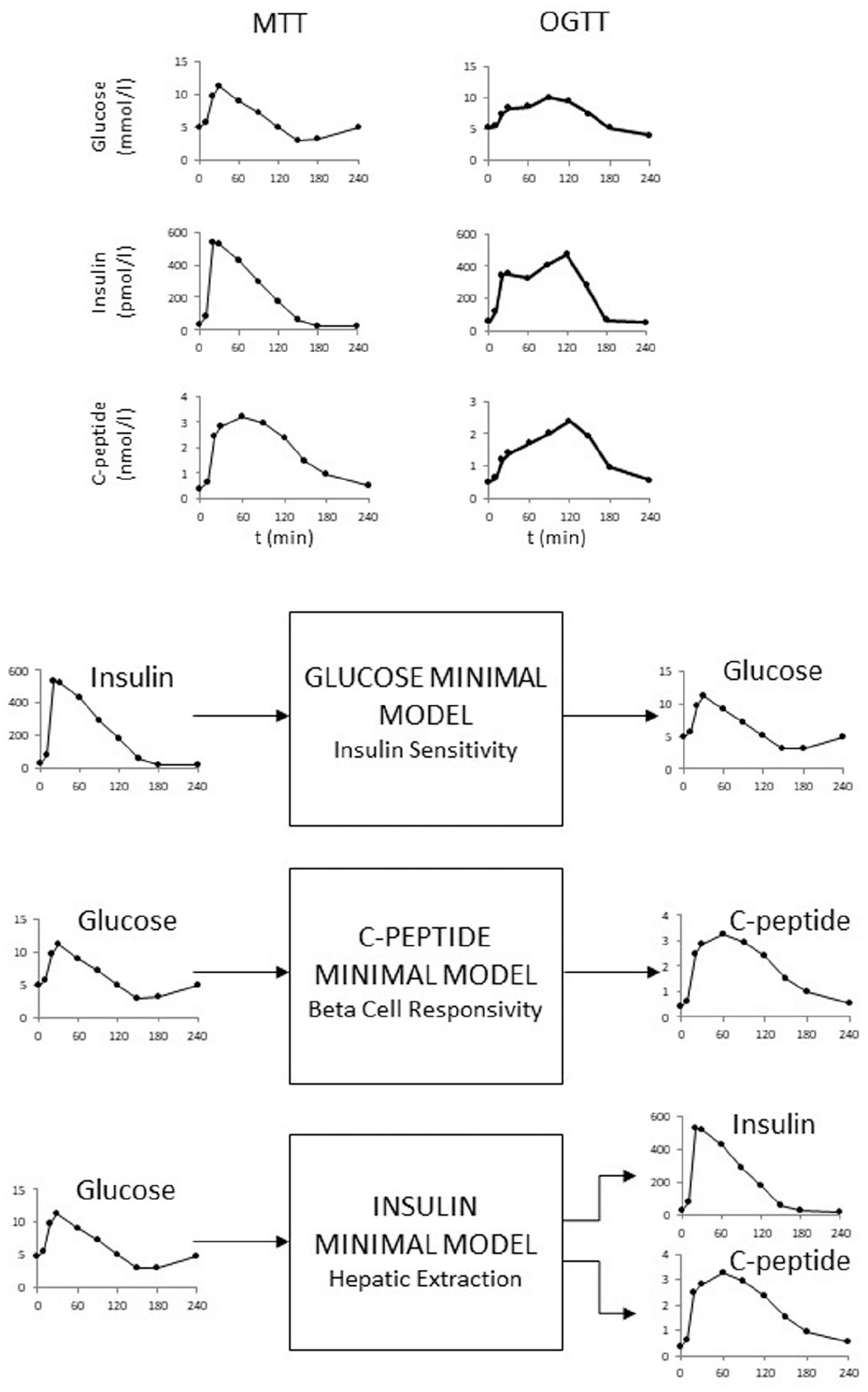
Top panel: Mixed meal (left) and OGTT(right) plasma glucose (top), insulin (middle) and C-peptide (bottom) in the same subject. Bottom panel: Partition analysis of the system allows to separately estimate insulin sensitivity, beta-cell responsivity and hepatic extraction without the confounding effect of the 2 other parameters. Relevant input and output signals of the 3 models are shown (adapted from ³⁵ ).

Figure 1 shows the recommended MTT/OGTT 10-sample schedule (0, 10, 20, 30, 60, 90, 120, 150, 180, 240 min) but 8-samples (without 150 and 240 min) still provide accurate results in subjects without diabetes at the individual level. If indices only in large population studies are needed, a 7-sample schedule can be used in subjects without diabetes and with prediabetes. ⁴¹

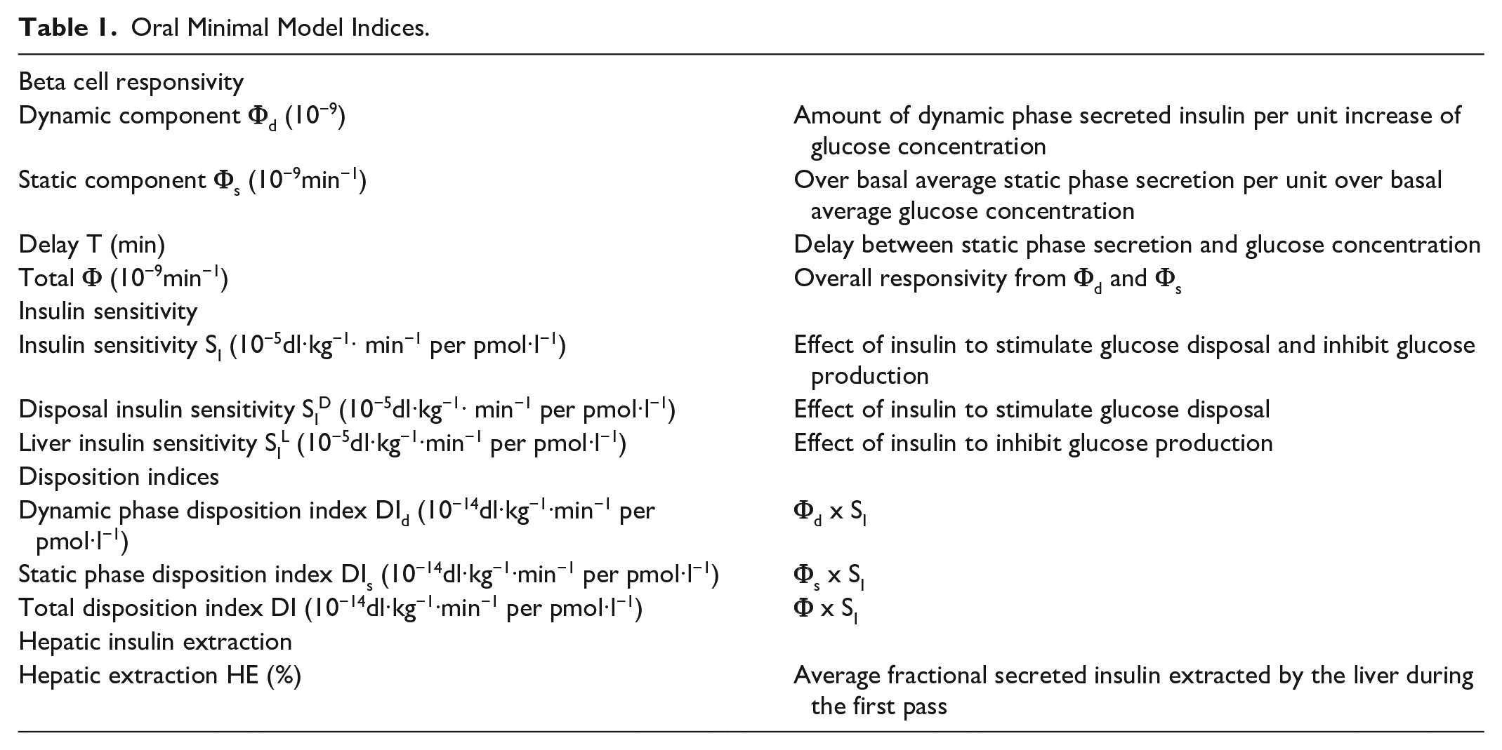
Table 1 summarizes the parameters of the oral minimal method.

Table 1.

Oral Minimal Model Indices.

Beta cell responsivity
Dynamic component Φd (10−9)	Amount of dynamic phase secreted insulin per unit increase of glucose concentration
Static component Φs (10−9min−1)	Over basal average static phase secretion per unit over basal average glucose concentration
Delay T (min)	Delay between static phase secretion and glucose concentration
Total Φ (10−9min−1)	Overall responsivity from Φd and Φs
Insulin sensitivity
Insulin sensitivity SI (10−5dl·kg−1· min−1 per pmol·l−1)	Effect of insulin to stimulate glucose disposal and inhibit glucose production
Disposal insulin sensitivity SID (10−5dl·kg−1· min−1 per pmol·l−1)	Effect of insulin to stimulate glucose disposal
Liver insulin sensitivity SIL (10−5dl·kg−1·min−1 per pmol·l−1)	Effect of insulin to inhibit glucose production
Disposition indices
Dynamic phase disposition index DId (10−14dl·kg−1·min−1 per pmol·l−1)	Φd x SI
Static phase disposition index DIs (10−14dl·kg−1·min−1 per pmol·l−1)	Φs x SI
Total disposition index DI (10−14dl·kg−1·min−1 per pmol·l−1)	Φ x SI
Hepatic insulin extraction
Hepatic extraction HE (%)	Average fractional secreted insulin extracted by the liver during the first pass

The Glucose Minimal Model

The glucose minimal model is shown in Figure 2 (upper panel). The gastrointestinal tract is the new element with respect to the IVGTT minimal model. Given the smoother oral vs IVGTT time course of plasma glucose and insulin, a single compartment model describes accurately glucose kinetics (while a 2 compartment model is needed to describe IVGTT in their integrity^38,42).

Figure 2.

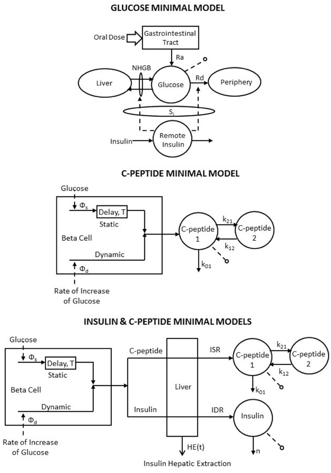
The oral glucose minimal models which allow to estimate insulin sensitivity (top panel), beta-cell responsivity (middle panel) and hepatic insulin extraction (bottom panel (adapted from ³⁵ ).

Denoting by Q the plasma glucose mass, Rd the rate of plasma glucose disappearance, Ra the rate of glucose appearance in plasma from the oral input and NHGB the net hepatic glucose balance, the model and the measurement equations are:

$$\{\begin{array}{l}\stackrel{.}{Q}(t)=-Rd(t)+NHGB(t)+Ra(t)Q(0)=Q_b\\ G(t)=\frac{Q(t)}{V}\end{array}$$

(1)

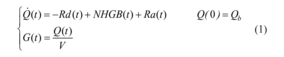
where G is plasma glucose concentration, V the glucose distribution volume and suffix b denotes basal value.

By assuming that Rd and NHGB are linearly dependent on Q, but modulated by insulin in a remote (vs plasma) compartment, as proposed in, ³⁰ one obtains: ⁴³

$$\{\begin{array}{ll}\stackrel{.}{Q}(t)=-\left[S_G+X(t)\right]\cdot Q(t)+S_G\cdot Q_b+Ra(\mathrm{\alpha },t)\hfill & Q(0)=Q_b\hfill \\ \begin{array}{l}\stackrel{.}{X}(t)=-p_2\cdot X(t)+p_3\cdot \left[I(t)-I_b\right]\\ G(t)=\frac{Q(t)}{V}\end{array}\hfill & \begin{array}{l}X(0)=0\end{array}\hfill \end{array}$$

(2)

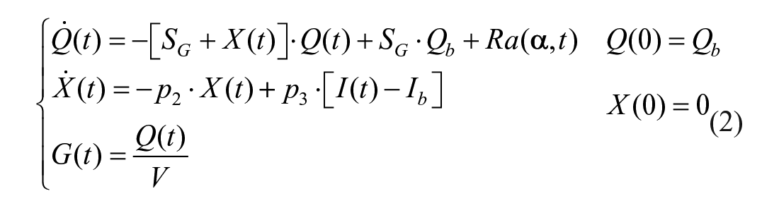
where S_G is fractional (ie, per unit distribution volume) glucose effectiveness measuring glucose ability per se to promote glucose disposal and inhibit NHGB, I plasma insulin concentration, X insulin action on glucose disposal and production, with p₂ and p₃ rate constants describing its dynamics and magnitude. Ra is described as a piecewise-linear function with known break-point t_i and unknown amplitude α_i:

$$Ra(\mathrm{\alpha },t)=\{\begin{array}{c}{\mathrm{\alpha }}_{i-1}+\frac{{\mathrm{\alpha }}_i-{\mathrm{\alpha }}_{i-1}}{t_i-t_{i-1}}\cdot (t_i-t_{i-1})for{t}_{i-1}\le t\le t_i,i=1,\cdot \cdot \cdot ,8\\ 0otherwise\end{array}$$

(3)

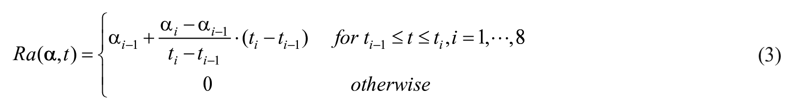
with α denoting [α_1, α₂,. . .α₈]^T.

Insulin sensitivity, S_I, is given by:

$$S_I=\frac{p_3}{p_2}\cdot V(\mathrm{dl}/\mathrm{kg}/\min \mathrm{per}\mu \mathrm{U}/\mathrm{ml})$$

(4)

A piecewise linear description for Ra with 8 parameters is sufficiently flexible to accommodate MTT/OGTT data. The input is plasma insulin with plasma glucose the output to be fitted by the model. Parameters α render the model not a priori uniquely identifiable because V is non-identifiable and S_G is non-uniquely identifiable. Thus, V and S_G are usually fixed to population values. To improve numerical identifiability, a Maximum a Posteriori Bayesian estimator is used by exploiting some prior on p₂ and a constraint on Ra, related to the total amount of glucose appearing in the circulation. S_I is precisely estimated with good precision and has been validated in a multiple tracer meal protocol ⁴⁴ and in an OGTT vs euglycemic glucose clamp study ⁴⁵ showing a correlation of 0.86 and 0.81, respectively. MTT S_I has been correlated with IVGTT S_I in the same subjects with correlation of 0.74. MTT S_I was also compared with OGTT S_I in 62 subjects ⁴⁶ with a correlation of r = 0.75, but S_I was significantly lower in MTT than OGTT.

Inter-subject variability of MTT S_I in healthy individuals is comparable to that of the IVGTT index, ⁴⁷ in particular its reproducibility (expressed as percent mean difference and coefficient of variation) were on average 8% and 23%, respectively.

The C-peptide Minimal Model

The model is shown in Figure 2 (middle panel): plasma C-peptide concentration is the output with glucose concentration as the input. ⁴⁸

The model is described by:

$$\{\begin{array}{l}{\stackrel{.}{q}}_1(t)=-\left(k_{01}+k_{21}\right)\cdot q_1(t)+k_{12}\cdot q_2(t)+ISR(t)q_1(0)=0\\ {\stackrel{.}{q}}_2(t)=-k_{12}\cdot q_2(t)+k_{21}\cdot q_1(t)q_2(0)=0\\ ISR(t)=y(t)+k_G\cdot \frac{dG(t)}{dt}\\ \stackrel{.}{y}(t)=-\frac{1}{T}\left[y(t)-\beta \cdot \left(G(t)-h\right)\right]y(0)=0\\ c_1(t)=\frac{q_1(t)}{V}\end{array}$$

(5)

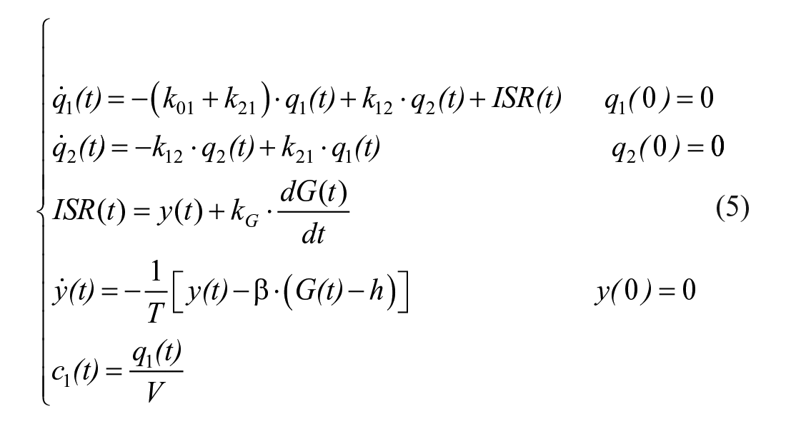
where q₁ and q₂ are respectively the above basal amount of C-peptide in the accessible and remote compartment (C-peptide 1 and 2 in Figure 2, middle panel), k₀₁, k₁₂ and k₂₁ are rate constants describing C-peptide kinetics, ISR is C-peptide (insulin) secretion rate, y is insulin provision (ie, the portion of synthesized insulin that reaches the cell membrane and can be released), and c₁ is above basal C-peptide plasma concentration. ISR is made up of 2 components: one proportional, through parameter k_G, to glucose rate of change (dG/dt), and one representing insulin release that, after a delay T, occurs proportionally to plasma glucose level above a threshold, h, through parameter β. The 2 components are termed dynamic, Φ_d (= k_G), and static, Φ_s (= β), responsivity indices. A single total responsivity index, Φ, which combines Φ_d and Φ_s, is often useful. The model is both a priori and numerically uniquely identifiable once C-peptide kinetic parameters (k₀₁, k₁₂ and k₂₁) are fixed using the population model. ²⁵ The picture is markedly different from that of the IVGTT, where the incretin effect is absent and the glucose signal is very different, with the derivative component only contributing during the first 2-3 minutes and the proportional component for the rest of test. This explains the fact that dynamic Φ_d and static Φ_s during an MTT are 250% greater than 1st phase, Φ₁, and 2nd phase, Φ₂, IVGTT indices in the same 204 individuals. ⁴⁰ Dynamic, Φ_d, and static, Φ_s, during an oral glucose challenge and IVGTT 1st, Φ₁, and 2nd, Φ_2, phase indices bear some relation (r = 0.52 for both indices), but they are likely determined by different cellular events.

MTT beta-cell responsivity indices were also compared with their OGTT counterparts in 62 subjects ⁴⁶ with good correlation, r = 0.71 for Φ_d, r = 0.73 for Φ_s, r = 0.74 for Φ, but the indices were significantly higher in MTT than OGTT.

It is an accepted notion that beta-cell function needs to be interpreted in light of the prevailing insulin sensitivity. One possibility is to resort to the disposition index (DI) paradigm, first introduced in 1981, ³⁴ and recently revisited,^47,49 where beta-cell function is multiplied by insulin sensitivity. This concept is clearly illustrated in Figure 3 (left panel). It is postulated that glucose tolerance of an individual is related to the product of beta-cell function and insulin sensitivity. In essence, different values of tolerance are represented by different hyperbolas, that is, DI = beta-cell function x insulin sensitivity = const. The DI was first introduced for IVGTT and has been extended to MTT/OGTT. Thus, disposition indices can be calculated by multiplying responsivity indices Φ_d, Φ_s, Φ by S_I to determine if the first phase, second phase and total beta-cell function are appropriate in light of the prevailing insulin sensitivity. For instance, while S_I was found to be significantly lower in MTT than OGTT and Φ significantly higher in MTT than OGTT, DI was the same, making it a good marker of glucose tolerance. ⁴⁶ The DI can also monitor in time the individual components of tolerance and assess different therapies (Figure 3, right panel).

Figure 3.

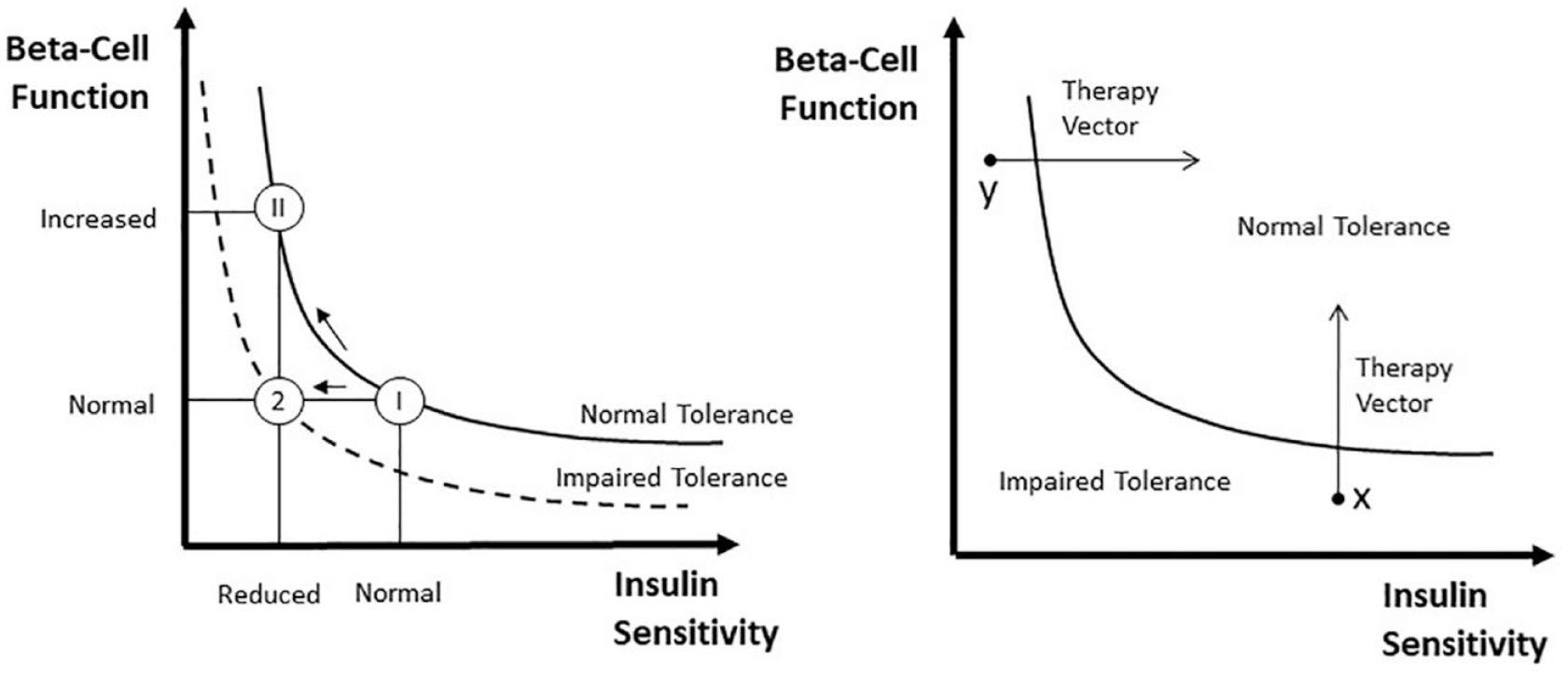
Schematic diagram to illustrate the importance of expressing beta-cell responsivity in relation to insulin sensitivity is illustrated by using the disposition index metric, that is, the product of beta-cell responsivity times insulin sensitivity is assumed to be a constant. Left panel: A normal subject (state I) reacts to impaired insulin sensitivity by increasing beta-cell responsivity (state II) while a subject with impaired tolerance does not (state 2). In state II beta-cell responsivity is increased but the disposition index is unchanged, and normal glucose tolerance is retained normal, while in state 2 beta-cell responsivity is normal but not adequate to compensate the decreased insulin sensitivity (state 2), and glucose intolerance is developed. Right panel: Impaired glucose tolerance can arise due to defects of beta-cell responsivity and/or defects of insulin sensitivity. In this hypothetical example, subject X is intolerant due to her/his poor beta-beta-cell function, while subject Y has poor insulin sensitivity. The ability to dissect the underlying physiological defects (insulin sensitivity or beta-cell responsivity) allows to optimize medical treatments (adapted from ³⁵ ).

However, the glucose-insulin feedback system is more complex than the simple hyperbola paradigm, that is, a more general DI could be DI = beta-cell function × (insulin sensitivity)^α = constant, where insulin sensitivity is raised to α. In addition, this simple concept hides several methodological issues addressed in, ⁴⁹ which, unless fully appreciated, could lead to errors in interpretation.

MTT Φ_d and Φ_s reproducibility was assessed in: ⁴⁷ percent mean difference was 1% and 7% and coefficient of variation was 31% and 18%, respectively.

An important addition to the MTT/OGTT parametric portrait is an index quantifying the effect of Glucagon-Like Peptide-1 (GLP-1)—a surrogate for the incretin effect ⁵⁰ - on insulin secretion. ⁵¹ This extension of the model accounting for the effect of exogenous GLP-1 infusion on insulin secretion was developed in. ⁵² In particular, the model ⁵² assumed that the above basal insulin secretion rate, ΔSR, is linearly modulated by GLP-1, through the GLP-1 sensitivity index π (% per pmol/l):

$$\mathrm{\Delta }{\mathrm{SR}}^{\mathrm{GLP1}}\left(\mathrm{t}\right)=\mathrm{\Delta }\mathrm{SR}\left(\mathrm{t}\right)\cdot \left[\pi \cdot \mathrm{GLP1}\left(\mathrm{t}\right)+1\right]$$

(6)

where GLP1(t) is the above basal intact hormone concentration.

π quantifies the ability of GLP-1 to enhance the over-basal insulin secretion, and is defined as the ratio between the average percent increase in over-basal insulin secretion and average GLP-1 plasma concentration.

The Insulin and C-peptide Minimal Model

Minimal models can also assess hepatic insulin extraction (Figure 2, bottom panel). Insulin secretion, ISR, can be assessed from the C-peptide model. Similarly, post-hepatic insulin delivery, IDR, can be assessed by employing an insulin model. In ⁵³ an insulin population model (along the line of ²⁵ ), allows to calculate insulin kinetic parameters from subject anthropometric characteristic in a population of subjects without diabetes. The model allows to reconstruct IDR. From ISR and IDR, both the time course of hepatic insulin extraction and an index numerically quantifying hepatic insulin extraction can be calculated:

$$HE(t)=\frac{ISR(t)-IDR(t)}{ISR(t)}=1-\frac{IDR(t)}{ISR(t)}$$

(7)

$$HE=\frac{{\int }_0^{T}ISR(t)-{\int }_0^{T}IDR(t)}{{\int }_0^{T}ISR(t)}=1-\frac{{\int }_0^{T}IDR(t)}{{\int }_0^{T}ISR(t)}$$

(8)

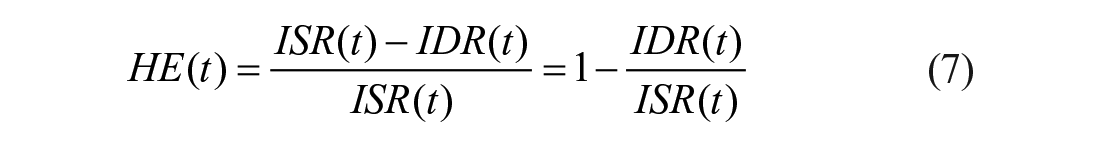
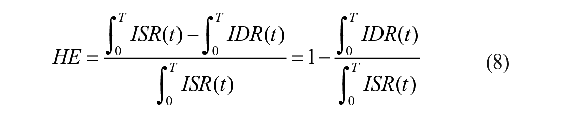
with T duration of the experiment.

The importance of adding HE to S_I and Φ for obtaining a more complete parametric portrait has been shown in several studies, for example.^54,55

Models at Work in Diabetes

The battery of oral glucose, C-peptide and insulin models have been used to study the effect of age and gender on glucose metabolism; ⁴⁰ the effect of anti-aging drugs; ⁵⁴ the influence of ethnicity;^55,56 insulin sensitivity and beta-cell function in people without diabetes ⁵⁷ and obese^58,59 adolescents, and children; ⁵⁹ the pathogenesis of prediabetes^46,60,61 and type 2 diabetes;^36,62 the diurnal pattern of insulin action and secretion in healthy ⁶³ and type 1 diabetes; ⁶⁴ the mechanism of insulin resistance in pregnancy; ⁶⁵ the effect of DPP4 inhibitors on insulin secretion; ⁶⁶ the effect of a bile acid sequestrant; ⁶⁷ caloric restriction;^68,69 vagal nerve blockade; ⁷⁰ genetic variation;^{71 -73} biliopancreatic diversion;^74,75 Roux-en-Y gastric bypass;^76,77 circadian misalignement;^78,79 oxytocin, ⁸⁰ and antidiabetic drugs ⁸¹ on insulin secretion and action.

Insulin Action Dissected by Tracer Modeling into Periphery and Liver

For reader convenience/information, most of the material reported in this section is taken from our review ³⁵ and a chapter of. ⁸²

If the oral glucose load is labelled with a glucose tracer (t), the exogenous glucose (G_exo), that is, the glucose concentration due to meal/OGTT only, can be calculate as:

$$G_{exo}\left(t\right)=t\left(t\right)\cdot \left(1+\frac{1}{TT{R}_{meal}}\right)$$

(9)

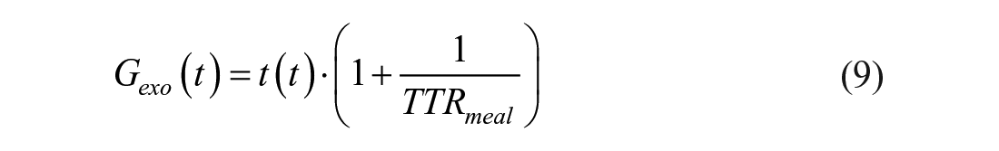
where TTR_meal is the tracer-to-tracee ratio in the meal/OGTT.

The endogenous glucose (G_end) can then be derived as G_end = G-G_exo, with G being the total glucose in plasma. In other words adding a tracer to the MTT/OGTT allows total glucose concentration to be segregated into its exogenous and endogenous components.

Disposal Insulin Sensitivity

G_exo measured in plasma is the result of the glucose rate of appearance coming from the MTT/OGTT, Ra, and the rate of glucose disposal, Rd (Figure 4). Thus, by fitting the model detailed in ⁸³ on G_exo and insulin one can estimate both Ra and disposal insulin sensitivity S_I^D, that is, the ability of insulin to enhance glucose utilization.

Figure 4.

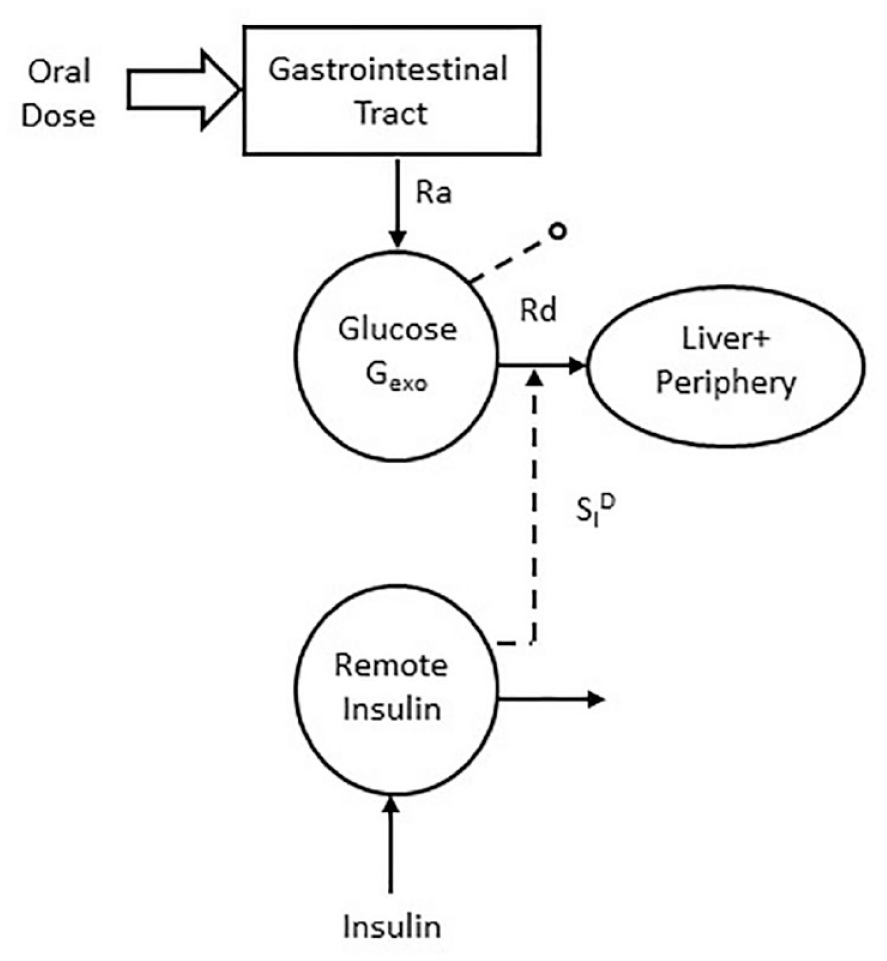
The labeled oral minimal model which allows to estimate disposal insulin sensitivity (adapted from ³⁵ ).

The model equations are:

$$\{\begin{array}{l}{\stackrel{.}{G}}_{exo}(t)=-\left[S_G^D+X^D(t)\right]\cdot G_{exo}(t)\\ +\frac{Ra(t,\mathrm{\alpha })}{V}{G}_{exo}(0)=0\\ {\stackrel{.}{X}}^{*}(t)=-p_2^D\cdot X^D(t)\\ +p_3^D\cdot \left[I(t)-I_b\right]X(0)=0\end{array}$$

(10)

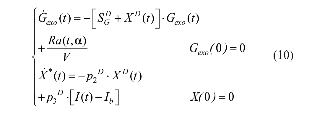
where S_G^D is fractional glucose effectiveness measuring glucose ability per se to promote glucose disposal, X^D insulin action on glucose disposal, with p₂^D and p₃^D rate constants describing respectively its dynamics and magnitude. Disposal insulin sensitivity is defined as:

$$S_I^D=\frac{p_3^D}{p_2^D}\cdot V(\mathrm{dl}/\mathrm{kg}/\min \mathrm{per}\mu \mathrm{U}/\mathrm{ml})$$

(11)

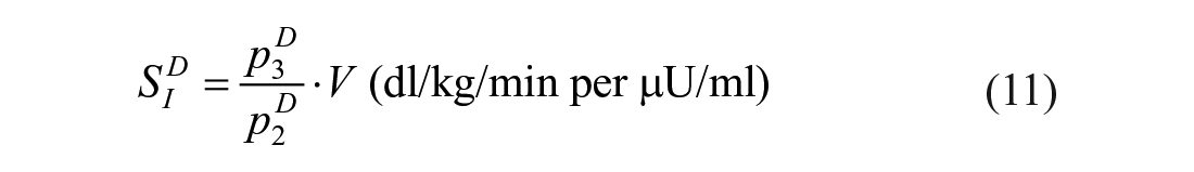
Ra is that already described for OMM (equation (3)).

The model has been validated first by comparing estimated Ra with a model-independent profile estimated with a multiple tracer experiment (Ra^ref, see Section 7.2.2) and S_I^D both with the same index obtained with the hot IVGTT minimal model ⁸⁴ fed with the model-independent Ra^ref. ⁸³ and with the disposal insulin sensitivity derived from labelled clamp. ⁴⁵ Correlation between S_I^D with disposal insulin sensitivity measured with the tracer enhanced euglycemic-hyperinsulinemic clamp technique was r = 0.70. ⁴⁵

Liver Insulin Sensitivity

Theoretically, by using the unlabelled and labelled models to measure, respectively, total (ie, periphery +liver) and peripheral indices, one should be able to calculate liver indices from the difference between the 2.

However, liver indices derived in this way are often unreliable (negative). This was found also during an IVGTT using the classic minimal model.^38,84-86 Caumo et al. ³⁸ suggested that these inconsistencies were to an inaccurate description of glucose and insulin effect on EGP. In fact, both the IVGTT and the oral minimal models assume that insulin action on the liver has the same time course of insulin action on glucose disposal. Moreover, EGP suppression includes a term linearly dependent on glucose and a term equal to the product of glucose concentration and insulin action, that is, insulin action on the liver is glucose-mediated. The minimal model EGP and alternative EGP descriptions have been assessed against virtually model-independent EGP profiles^87,88 and liver insulin sensitivity (S_I^L) and glucose effectiveness (GE^L) were estimated.

According to, ⁸⁸ EGP can be described as:

$$\begin{array}{l}EGP(t)=EG{P}_b-k_G\cdot \left[G(t)-G_b\right]-X^L(t)-X^{Der}(t)\\ EGP(0)=EG{P}_b\end{array}$$

(12)

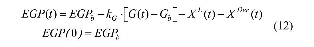
where EGP_b is basal endogenous glucose production, k_G is liver glucose effectiveness.

X^L is liver insulin action, defined as:

$$\{\begin{array}{l}{\stackrel{.}{X}}^L(t)=-k_1\cdot X^L(t)+k_1\cdot X^{\prime }(t)\\ X^L(0)=0\\ {\stackrel{.}{X}}^{\prime }(t)=-k_1\cdot \left[X^{\prime }(t)-k_2\cdot \left(I(t)-I_b\right)\right]\\ X^{\prime }(0)=0\end{array}$$

(13)

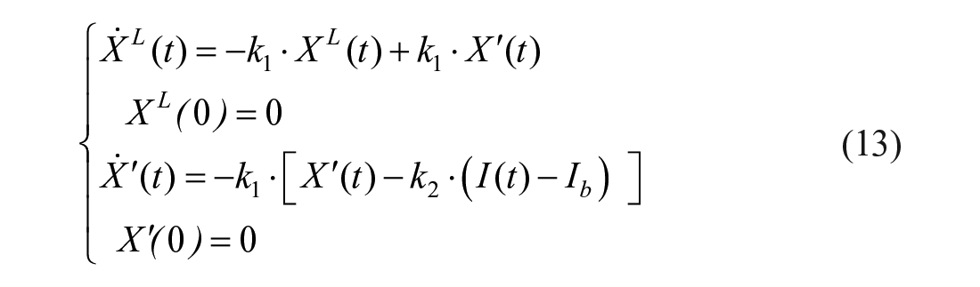
with k₁ accounting for the delay of liver insulin action vs plasma insulin, and k₂ a parameter governing its efficacy. X^Der is a surrogate of portal insulin, which anticipates insulin and glucose patterns, and was demonstrated to significantly improve model ability to fit the rapid suppression of EGP occurring immediately after a meal:

$$X^{Der}(t)=\{\begin{array}{l}{k}_{GR}\cdot \frac{dG(t)}{dt}if\frac{dG(t)}{dt}\ge 0\\ 0if\frac{dG(t)}{dt}<0\end{array}$$

(14)

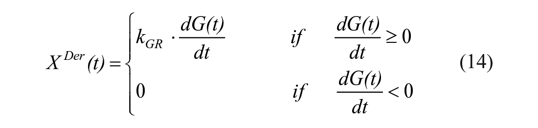
where k_GR is a parameter governing the magnitude of glucose derivative control.

An index of liver insulin sensitivity (S_I^L) can be derived from model parameters as follows:

$$S_I^L=-{\frac{\partial EGP}{\partial I}|}_{ss}\cdot \frac{1}{G_b}=\frac{k_2}{G_b}$$

(15)

where the symbol |_ss indicates that the derivative of EGP is calculated in steady state.

The model has been first assessed in healthy subjects. ⁸⁸ Then, it was validated by comparing S_I^L with liver insulin sensitivity measured with a tracer enhanced euglycemic-hyperinsulinemic clamp (S_I^Lclamp) in subjects with different degrees of glucose tolerance. ⁸⁹ S_I^Lclamp is derived from total and peripheral indices as:

$$S_I^{Lclamp}=S_I^{clamp}-S_I^{*clamp}$$

(16)

Correlation between S_I^Lclamp and S_I^L was good (r = 0.72, P < 0.0001), with S_I^Lmeal being lower than S_I^Lclamp (4.60 ± 0.64 vs 8.73 ± 1.07 10⁻⁴ dl/kg/min per μU/ml, P < 0.01). It is noteworthy that the correlation improved to 0.80, P < 0.001 in normal fasting glucose subjects, while it was lower in impaired fasting glucose subjects (r = 0.56, P = 0.11, likely due to the limited sample size).

The Single Tracer Oral Minimal Model

The new model describing EGP suppression after a meal has been incorporated into the oral glucose minimal model to see if S_I^L could be obtained from plasma concentrations measured after a single-tracer meal by describing both glucose production, P, and disposal, D (OMM^PD). ⁹⁰

Triple-tracer meal data of 2 databases (20 healthy and 60 subjects without diabetes and with prediabetes) were used in which a virtually model-independent EGP estimate was available (see Section 7.2.2). OMM^PD was identified on exogenous and endogenous glucose concentrations, providing indices of S_I^L, S_I^D and EGP time course.

The estimated S_I^L well compared with that derived directly from EGP data. ⁸⁸ Since the model is not able to assess basal EGP (EGP_b), only the ratio (EGP/EGP_b) can be estimated together with S_I^Land S_I^D.

Multiscale Glucose Tracer Modeling: Insulin Action on Skeletal Muscle Processes

For reader convenience/information, most of the material reported in this section is taken from our review. ¹

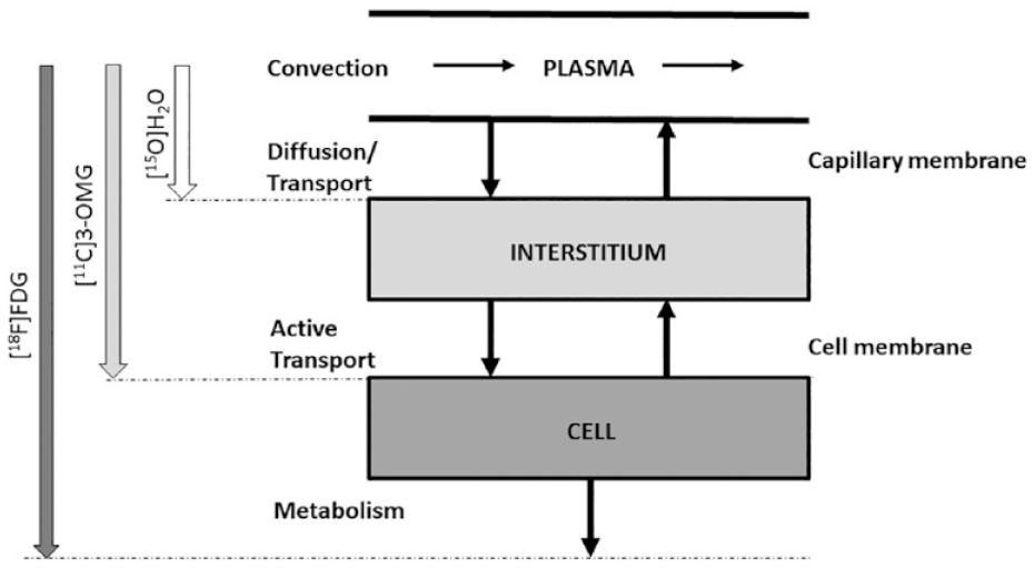
While whole-body models can provide important quantitative information on insulin action, it is important but at the same time remarkably difficult, to noninvasively measure the effect of insulin on glucose transport and metabolism at the organ level. A crucial target tissue of glucose metabolism is the skeletal muscle. Impaired insulin action in muscle is a well-recognized characteristic of a number of metabolic diseases, including type 2 diabetes, obesity, hypertension, and cardiovascular disease. Understanding its causes requires to segregate and quantify in situ the major individual steps of glucose processing, particularly those of glucose delivery, transport in and out of the cell, and phosphorylation (Figure 5).

Figure 5.

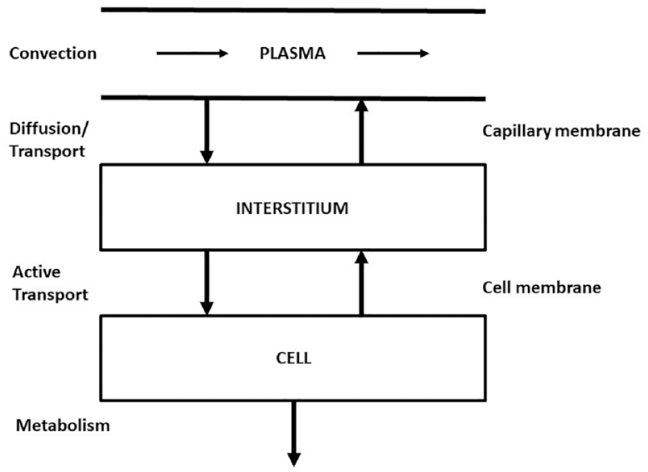
Skeletal muscle major glucose processes: diffusion to/from the intersitium, active transport in and out of the cell, and phosphorylation/metabolism.

The classical experimental approach is based on the multiple tracer dilution,^1,91 which consists of the simultaneous injection, upstream of the organ, of more than one tracer to allow the separate monitoring of the individual steps of glucose metabolism. In the 2000s, the positron emission tomography (PET) noninvasive imaging technique was proposed which can provide highly specific and rich biochemical information if applied in dynamic mode, that is, sequential tissue images acquired following a bolus injection of tracer.

Multiple tracer dilution data can be interpreted with both linear distributed parameter (see reviews ¹⁶ and ⁹² ) and compartmental organ models. ⁹³ The only application to glucose metabolism of distributed parameter models has been in an isolated and perfused heart. ¹ In contrast, compartmental organ models have been more intensively applied to interpret multiple tracer dilution data in the human skeletal muscle. A compartmental model has been proposed^94,95describing the transmembrane transport of glucose, that is, into and out of the cell. This model has been extended ⁹⁶ to describe the kinetics of a third tracer, permeant nonmetabolizable, thus allowing to quantify not only the rate constants of transport and phosphorylation, but also the bidirectional glucose flux through the cell membrane, the phosphorylation flux, and the intracellular concentration, in subjects with and without diabetes and obese.^97,98 This allowed to show that insulin control on both transmembrane transport and phosphorylation flux in subjects with diabetes is much less efficient with respect to subjects without diabetes.

PET data can be analyzed by regional compartmental modeling. The brain glucose model by Sokoloff et al. ⁹⁹ has been a landmark. The selected tracer for studying glucose metabolism in skeletal muscle (but also in the brain and myocardium) is [ ¹⁸ F] fluorodeoxyglucose ([ ¹⁸ F]FDG), a glucose analog. The ideal tracer would be [ ¹¹ C–glucose], but the interpretative model by having to account for all metabolic products along the glycolysis and glycogenosynthesis pathways cannot be resolved. The advantage of [ ¹⁸ F]FDG is that a simpler model can be adopted. In fact, [ ¹⁸ F]FDG once in the tissue, similarly to glucose, can either be transported back to plasma or can be phosphorilated to [ ¹⁸ F]FDG-6-phosphate, [ ¹⁸ F]FDG-6-P. The advantage is that [ ¹⁸ F]FDG-6-P is trapped in the tissue and released very slowly. In other words, [ ¹⁸ F]FDG-6-P cannot be metabolized further, while glucose-6-P does so along the glycolysis and glycogenosynthesis pathways. The major disadvantage of [ ¹⁸ F]FDG is the necessity to correct for the differences in transport and phosphorylation between the analog [ ¹⁸ F]FDG and glucose. A correction factor called lumped constant (LC) can be employed to convert [ ¹⁸ F]FDG fractional uptake (but not the [ ¹⁸ F]FDG transport rate parameters) to that of glucose. LC values in human skeletal muscle are available.^100,101 The interpretative model is a 4-compartment model (plasma, extracellular, tissue [ ¹⁸ F]FDG, and [ ¹⁸ F]FDG-6-phosfate) with 5 rate constants. ¹⁰² The model (Figure 6) is described by:

Figure 6.

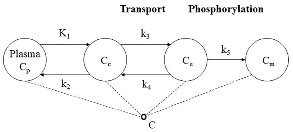
The 5k model of [ ¹⁸ F]FDG in skeletal muscle: C_p is [ ¹⁸ F]FDG plasma arterial concentration, C_c extracellular concentration of [ ¹⁸ F]FDG normalized to tissue volume, C_e [ ¹⁸ F]FDG tissue concentration, Cm [ ¹⁸ F]FDG—6—P tissue concentration, C total ¹⁸ F activity concentration in the ROI, K₁ [ml/ml/min] and k₂ [min⁻¹] the exchange between plasma and extracellular space, k₃ [min⁻¹] and k₄ [min⁻¹] transport in and out of cell, k₅ [min⁻¹] phosphorylation.

$$\begin{array}{l}{\stackrel{.}{\mathrm{C}}}_{\mathrm{c}}{\left(\mathrm{t}\right)=\mathrm{K}}_1{\mathrm{C}}_{\mathrm{p}}{\left(\mathrm{t}\right)-(\mathrm{k}}_2+{\mathrm{k}}_3\left){\mathrm{C}}_{\mathrm{c}}{\left(\mathrm{t}\right)+\mathrm{k}}_4{\mathrm{C}}_{\mathrm{e}}\left(\mathrm{t}\right){\mathrm{C}}_{\mathrm{c}}\right(0)=0\\ {\stackrel{.}{\mathrm{C}}}_{\mathrm{e}}{\left(\mathrm{t}\right)=\mathrm{k}}_3{\mathrm{C}}_{\mathrm{c}}{\left(\mathrm{t}\right)-(\mathrm{k}}_4+{\mathrm{k}}_5\left){\mathrm{C}}_{\mathrm{e}}\right(\mathrm{t}\left){\mathrm{C}}_{\mathrm{e}}\right(0)=0\\ {\stackrel{.}{\mathrm{C}}}_{\mathrm{m}}{\left(\mathrm{t}\right)=\mathrm{k}}_5{\mathrm{C}}_{\mathrm{e}}\left(\mathrm{t}\right){\mathrm{C}}_{\mathrm{m}}\left(0\right)=0\end{array}$$

(17)

$${\mathrm{C}\left(\mathrm{t}\right)=(1-\mathrm{V}}_{\mathrm{b}}\left)\left({\mathrm{C}}_{\mathrm{c}}{\left(\mathrm{t}\right)+\mathrm{C}}_{\mathrm{e}}{\left(\mathrm{t}\right)+\mathrm{C}}_{\mathrm{m}}\left(\mathrm{t}\right)\right){+\mathrm{V}}_{\mathrm{b}}{\mathrm{C}}_{\mathrm{b}}\right(\mathrm{t})$$

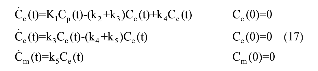
where C_p is [ ¹⁸ F]FDG plasma arterial concentration, C_c is extracellular concentration of [ ¹⁸ F]FDG normalized to tissue volume, C_e [ ¹⁸ F]FDG is tissue concentration, C_m [ ¹⁸ F]FDG-6-P is tissue concentration, C total ¹⁸ F is activity concentration in the ROI, K₁ [ml/ml/min] and k₂ [min⁻¹] are the exchanges between plasma and extracellular space, k₃ [min⁻¹] & k₄ [min⁻¹] are the rates of transport in and out of cell, and k₅ [min⁻¹] is the rate of phophorylation. V_b is the fractional blood volume in the region of interest, and C_b is the whole blood tracer concentration. From the model one can calculate the fractional uptake of [ ¹⁸ F]FDG, K [ml/ml/min]:

$$\mathrm{K}=\frac{{\mathrm{K}}_1{\mathrm{k}}_3{\mathrm{k}}_5}{{\mathrm{k}}_2{\mathrm{k}}_4{+\mathrm{k}}_2{\mathrm{k}}_5{+\mathrm{k}}_3{\mathrm{k}}_5}$$

(18)

and, by using LC value and the glucose basal plasma concentration value, the glucose fractional uptake.

To move from FDG to glucose, a multi-tracer PET method is needed, ¹⁰³ which allows the simultaneous assessment of blood flow, glucose transport, and phosphorylation in the skeletal muscle. The method employs 3 different PET tracers (Figure 7) injected at different times, and allows to quantify blood flow from [ ¹⁵ O]H₂O images with one- compartment 2-rate constant model; glucose transport from [ ¹¹ C]3-OMG images with a 3 compartment 4-rate constant model, and, finally, glucose phosphorylation by combining [ ¹⁸ F]FDG fractional uptake with [ ¹¹ C]3-OMG rate constants. The [ ¹¹ C]-3-OMG model is a simpler version of that of equation (17), since [ ¹¹ C]3-OMG is not phosphorylated. This multi-tracer model has provided important insight on insulin action on muscle unit processes; in particular, it was shown that: glucose transport from plasma into interstitial space is not affected by insulin; insulin significantly increases both glucose transport and phosphorylation; predominately oxidative muscles (soleus) have higher perfusion and higher capacity for glucose phosphorylation than less oxidative muscles (tibialis).

Figure 7.

The 3 PET tracer protocol to study glucose diffusion through capillary membrane, active transport into the cells and metabolism.

Multiscale Insulin Modeling: Insight into Secretory Cellular Events

For reader convenience/information, most of the material reported in this section is taken from our review. ²

The models of beta-cell function provide a quantitative assessment of beta-cell function at the whole-body level. To gain a mechanistic insight into the cellular phenomena responsible for insulin secretion, one has to move down in the hierarchical system structure.

The starting point is the landmark model by Grodsky ³² (Figure 8, left panel), briefly described in Section 2, and updates of this model based on data of cell-to-cell heterogeneity with respect to their activation threshold ¹⁰⁴ and Ca²⁺ imaging experiments.^105,106 This new subcellular model ¹⁰⁷ describes the dynamics of granule pools in the entire pancreatic population of beta-cells (Figure 8, right panel). Granules mobilize from a reserve pool to a pool of “docked” granules at the plasma membrane. The granules can mature further (priming) to gain release competence and enter the “readily releasable pool” (RRP). Calcium influx then triggers exocytosis and insulin release from the RRP. RRP is heterogeneous, that is, only granules residing in cells with a threshold for calcium activity below the ambient glucose concentration are allowed to fuse. Thanks to RRP heterogeneity, the model can describe all the classical glucose stimuli, including staircase glucose infusion protocol.

Figure 8.

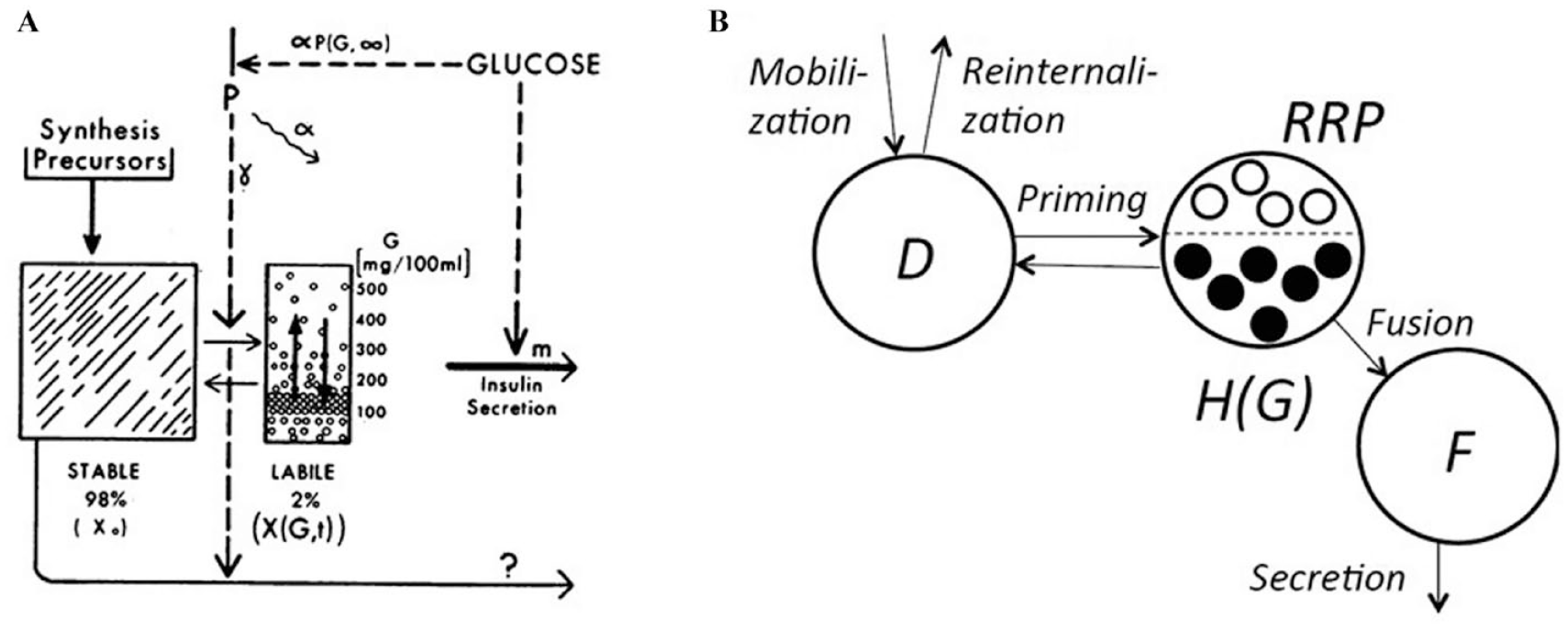
Left panel: Grodsky’s ³² model with a large reserve pool and a small labile pool of insulin packets with different thresholds. Right panel: The model ¹⁰⁴ with a pool of docked insulin granules (D), a readily releasable pool (RRP) and a pool of fused granules (F) releasing insulin. The model assumes that beta-cells have different activation threshold with respect to the glucose concentration (G) by distinguishing between RRP granules in active cells (denoted H(G), filled circles) and in silent cells (open circles) (adapted from ² and ¹⁰⁴ ).

Using multiscale modeling the relation between the beta-cell function minimal model indices and the subcellular events described in the mechanistic model have been investigated. ¹⁰⁸ Both the oral and the IVGTT minimal secretion models can be interpreted in the light of this cellular model. The analysis revealed that the first-phase IVGTT and the dynamic oral secretion both reflect the amount of readily releasable insulin, but also that the dynamic secretion is shaped by the threshold distribution for cell activation as well as the dynamics of mobilization and docking. Second phase IVGTT and static oral secretion reflect a combination of mobilization, docking, priming and recruitment of new cells. A first attempt to a better understanding of the mechanistic effects of incretins was done in ¹⁰⁹ by including GLP-1 in the oral minimal model.

A Flux Portrait of the Glucose System: Tracers to Measure Simple and Complex Carbohydrate Postprandial Metabolism

Measuring the postprandial glucose turnover is not easy. ¹¹⁰ At variance with the fasting state, after a meal, glucose concentration is not in steady state and is the results of Ra_meal, EGP, and Rd pattern.

The first attempt to solve this difficult task was that of Steele et al. ¹⁷ . They proposed to label the ingested glucose with one glucose tracer and intravenously infusing a second tracer at a constant rate. Unfortunately, subsequent studies have shown that although this approach is technically simple, the marked changes in plasma tracer-to-tracee ratio, if stable tracers are used, or specific activity, if a radioactive tracer is used, introduce a substantial error in the calculation of Ra_meal, EGP, and Rd, thereby leading to incorrect and at times misleading results. ¹¹¹ This is due to the so called nonsteady state error, which is very pronounced after a meal perturbation if the tracer is infused constantly. To minimize such error, Basu and coworkers have proposed a more complex experimental technique called the triple tracer method, presented later in this paragraph, which implements the so called tracer-to-tracee clamp technique. ⁸⁷

The theory behind the 2 techniques is described in detail below.

When the system is in steady state, the rate of glucose entering the circulation (Ra) equals the rate of glucose leaving the system (Rd). If one starts to infuse the glucose tracer at a constant rate (INF), after a while, also the tracer will be in steady state, and so is also the tracer (g) to tracee (G) ratio (TTR = g/G).

It can easily been shown that one has:

$$Ra=Rd=\frac{INF}{g_{ss}V}{G}_{ss}V=\frac{INF}{TTR}$$

(19)

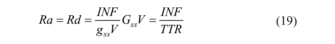
In other words, the estimate of Ra and Rd is model-independent.

In case of food ingestion, the estimation of Ra and Rd becomes more difficult. First, Ra and Rd are no longer equal and both are changing over time, resulting in a nonconstant TTR. In addition, Ra now equals the sum of Ra_meal and EGP, which are also changing with time. ¹¹⁰

In this case, one needs to specify both the structure (one compartment, 2 compartment, multi-compartment. . .) and which parameters are time-varying and these choices have an impact on the glucose fluxes estimate.

For the glucose system the most popular assumptions are that the model is a one- ¹⁷ or a 2-compartment ¹⁹ model and that the time-varying parameter is the fractional clearance rate, since it is known that it is controlled by insulin concentration, which is likely to vary after a meal.

The Intravenous Glucose Infusion Case

For sake of simplicity, let first consider the simpler case of exogenous glucose intravenous infusion (GIR), instead of a meal, so that GIR is known and only EGP and Rd have to be estimated. In other words, one will estimate Ra(t) = GIR(t)+EGP(t) and then calculate EGP(t) by subtracting the known GIR(t) from the estimated Ra(t). Rd(t) will be then calculated from the model using the mass balance equation. Let also start with a single compartment description with time-varying fractional clearance rate (k(t)) proposed by Steele et al. ¹⁷

Given that the system is not in steady state, the model of the tracee is:

$$\{\begin{array}{c}\begin{array}{l}\stackrel{.}{Q}\left(t\right)=Ra\left(t\right)-Rd\left(t\right)\\ =Ra\left(t\right)-k\left(t\right)Q\left(t\right)Q\left(0\right)=Q_{ss}=G_{ss}V\end{array}\\ G\left(t\right)=\frac{Q\left(t\right)}{V}\end{array}$$

(20)

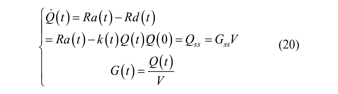
Thanks to the tracer-to-tracee indistinguishability principle, one has:

$$\{\begin{array}{c}\stackrel{.}{q}\left(t\right)=INF-rd\left(t\right)=INF-k\left(t\right)q\left(t\right)q\left(0\right)=0\\ g\left(t\right)=\frac{q\left(t\right)}{V}\end{array}$$

(21)

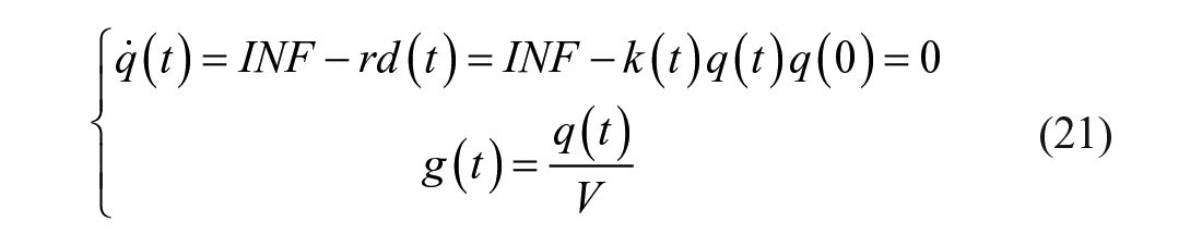
The fractional clearance rate k(t) is derived from equation (21):

$$k\left(t\right)=\frac{INF}{q\left(t\right)}-\frac{\stackrel{.}{q}\left(t\right)}{q\left(t\right)}$$

(22)

By substituting k(t) of equation (22) into equation (20) and rearranging it, one obtains:

$$\begin{array}{l}Ra\left(t\right)=\frac{INF}{TTR\left(t\right)}-\frac{q\left(t\right)}{TTR\left(t\right)}\cdot \frac{dTTR\left(t\right)}{dt}=\\ \frac{INF}{TTR\left(t\right)}-\frac{g\left(t\right)}{TTR\left(t\right)}V\cdot \frac{dTTR\left(t\right)}{dt}\end{array}$$

(23)

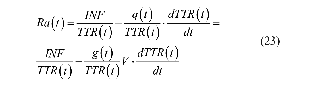
where we have used the relationship

$$TTR\left(t\right)=\frac{g\left(t\right)}{G\left(t\right)}=\frac{q\left(t\right)}{Q\left(t\right)}$$

Steele et al. ¹¹² realized that TTR measured in the plasma does not represent that in the liver, interstitial fluid, and other compartments. To circumvent this problem, they used a nonhomogenous compartment model and assumed that the “effective” volume was only a fraction of the total body volume of distribution of glucose V, indicated as pV, with p ranging from 0.5 to 0.8:^113-115

$$Ra\left(t\right)=\frac{INF}{TTR\left(t\right)}-\frac{g\left(t\right)}{TTR\left(t\right)}pV\cdot \frac{dTTR\left(t\right)}{dt}$$

(24)

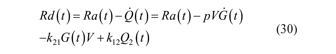
EGP and Rd are then calculated as:

$$EGP\left(t\right)=Ra\left(t\right)-GIR\left(t\right)$$

(25)

$$Rd\left(t\right)=Ra\left(t\right)-\stackrel{.}{Q}\left(t\right)=Ra\left(t\right)-pV\stackrel{.}{G}\left(t\right)$$

(26)

On the other hand, if one assumes that the system is described by a 2 compartment model and that only k₀₁(t) is a time-varying parameter, ¹⁹ one has:

$$\{\begin{array}{c}\begin{array}{c}\begin{array}{l}{\stackrel{.}{Q}}_1\left(t\right)=Ra\left(t\right)-\left[k_{01}\left(t\right)+k_{21}\right]Q_1\left(t\right)\\ +k_{12}{Q}_2\left(t\right)Q_1\left(0\right)=Q_{ss}=G_{ss}V\end{array}\\ {\stackrel{.}{Q}}_2\left(t\right)=k_{21}{Q}_1\left(t\right)-k_{12}{Q}_2\left(t\right)Q_2\left(0\right)=G_{ss}V\frac{k_{21}}{k_{12}}\end{array}\\ G\left(t\right)=\frac{Q_1\left(t\right)}{V}\end{array}$$

(27)

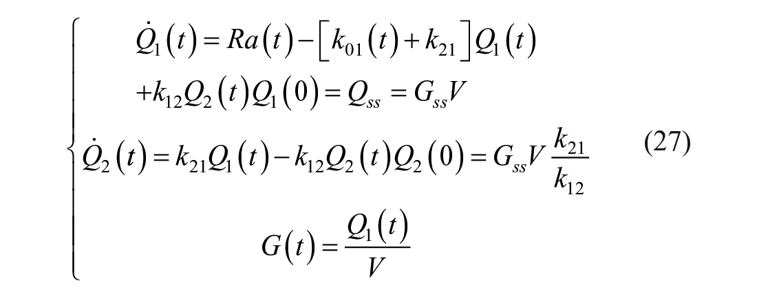
and the tracer model is:

$$\{\begin{array}{c}\begin{array}{c}{\stackrel{.}{q}}_1\left(t\right)=INF-\left[k_{01}\left(t\right)+k_{21}\right]q_1\left(t\right)+k_{12}{q}_2\left(t\right)q_1\left(0\right)=0\\ {\stackrel{.}{q}}_2\left(t\right)=k_{21}{q}_1\left(t\right)-k_{12}{q}_2\left(t\right)q_2\left(0\right)=0\end{array}\\ g\left(t\right)=\frac{q_1\left(t\right)}{V}\end{array}$$

(28)

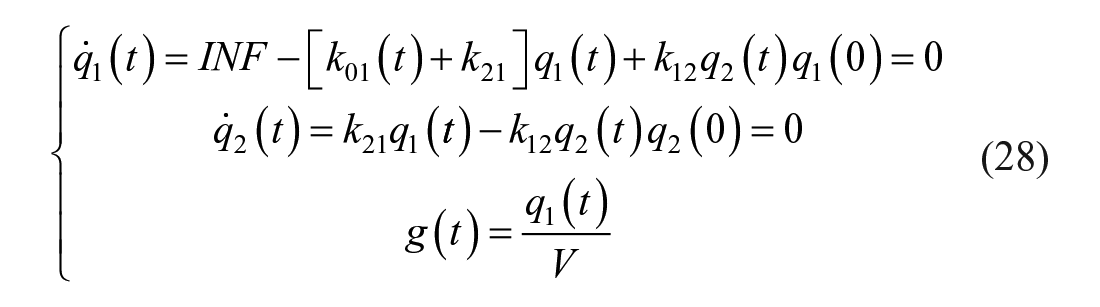
Paralleling what done for Steele et al model, if one derives k₀₁(t) from equation (28) and substitute it into 27, one obtains:

$$\begin{array}{l}Ra\left(t\right)=\frac{INF}{TTR\left(t\right)}-\frac{g\left(t\right)}{TTR\left(t\right)}V\cdot \frac{dTTR\left(t\right)}{dt}\\ +k_{21}\left(\frac{q_2\left(t\right)}{TTR\left(t\right)}-Q_2\left(t\right)\right)\end{array}$$

(29)

where $TTR\left(t\right)=\frac{g\left(t\right)}{G\left(t\right)}=\frac{q_1\left(t\right)}{Q_1\left(t\right)}$ .

EGP is then calculated as in equation (25), while Rd, according to the 2-compartment model, is:

$$\begin{array}{l}Rd\left(t\right)=Ra\left(t\right)-\stackrel{.}{Q}\left(t\right)=Ra\left(t\right)-pV\stackrel{.}{G}\left(t\right)\\ -k_{21}G\left(t\right)V+k_{12}{Q}_2\left(t\right)\end{array}$$

(30)

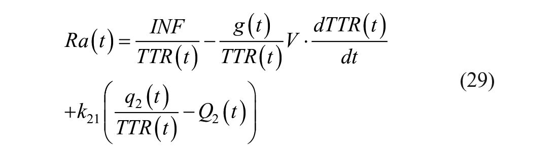
By comparing equations (24) and (29), it is evident that the estimate of Ra(t) is model-dependent and so are EGP(t) and Rd(t). One can argue that the accuracy of the flux estimate can be improved by postulating increasingly complex models (eg, those that account for differences in the rates of equilibration of glucose and onset of action of insulin in the liver, muscle, and various other tissues in people with or without diabetes). However, the increased complexity of the model has to be balanced against increased difficulty in accurately identifying model parameters.

Luckily, looking at equations (24) and (29), it is also clear that the closer is TTR(t) to a constant (clamped TTR) the smaller are the second term in equation (24) and the second and third terms in equation (29). Therefore, the maintenance of TTR in steady state by an appropriate tracer experiment design enables a quasi model-independent measurement of Ra(t), EGP(t), and Rd(t).

The question now become: is there a smart way to infuse the tracer so that TTR becomes virtually constant?

The answer is yes: since TTR is the ratio between the infused tracer and the total glucose concentration, the better way to clamp TTR is to infuse the tracer by mimicking the expected pattern of Ra(t), that is, constantly infusing the tracer before the exogenous infusion starts, following the expected pattern EGP thereafter, and labeling GIR.

The Mixed Meal (MTT) and the Oral Glucose (OGTT) Tolerance Test

In the case of an unknown exogenous input, for example, during an MTT or an OGTT, one needs at least one tracer mixed with the meal (oral load) to segregate exogenous from endogenous glucose in plasma and another tracer to be infused intravenously to calculate k(t), in case of Steele et al. ¹⁷ model, or k₀₁(t) in case of Radziuk ¹⁹ model. This minimal configuration is called the dual tracer method.

The dual tracer method

Let’s call tracer1 (t₁) the tracer mixed in the meal, with a TTR in the meal equal to TTR_meal, and tracer2 (t₂) the tracer infused intravenously with a constant rate (Figure 9, left panel).

Figure 9.

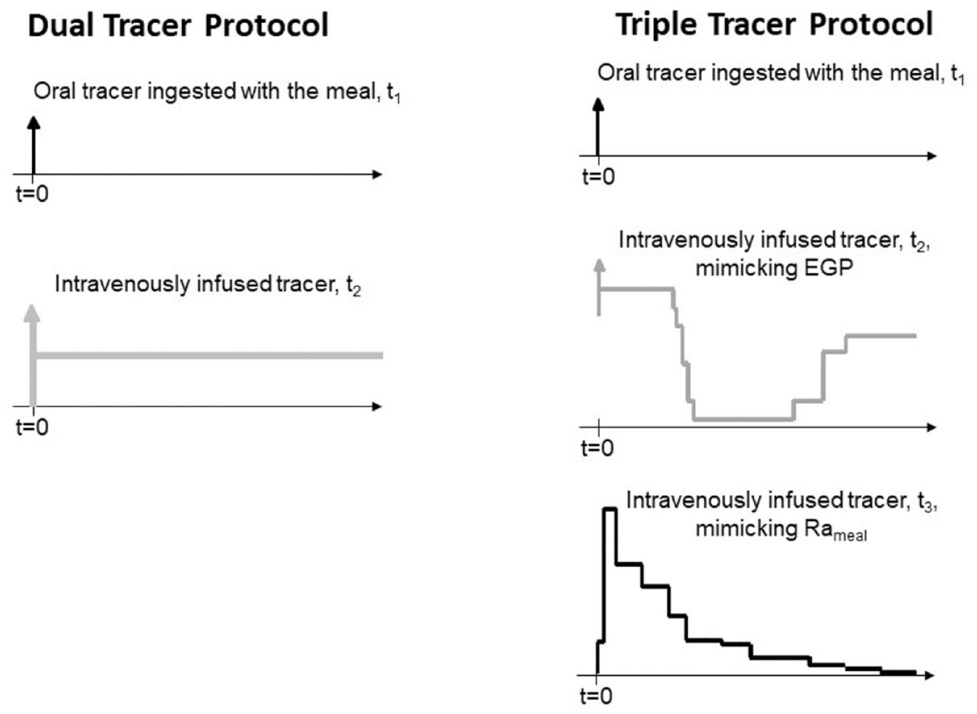
Scheme of the dual (left) and the triple tracer (right panel) protocol. In the dual tracer protocol the first tracer is mixed with the meal and the second one is infused intravenously with a constant rate. In the triple tracer protocol the first tracer is mixed with the meal, the second one is infused intravenously trying to mimic the expected pattern of EGP and the third one is infused intravenously trying to mimic the expected pattern of Ra_meal.

Exogenous glucose (G_exo), both labeled and unlabeled, can be derived from t₁ concentration and TTR_meal:

$$G_{exo}\left(t\right)=t_1\left(t\right)\cdot \left(1+\frac{1}{TT{R}_{meal}}\right)$$

(31)

Endogenous glucose (G_end) is derived by subtracting exogenous and i.v. infused tracer concentration (in case of a stable isotope) from total glucose (G):

$$G_{end}\left(t\right)=G\left(t\right)-G_{exo}\left(t\right)-t_2\left(t\right)$$

(32)

Let now define $TT{R}_{exo}\left(t\right)=\frac{t_2\left(t\right)}{G_{exo}\left(t\right)}$ and $TT{R}_{end}\left(t\right)=\frac{t_2\left(t\right)}{G_{end}\left(t\right)},$ then meal rate of appearance Ra_meal and EGP can be derived with Steele equation as:

$$R{a}_{meal}\left(t\right)=\frac{INF\left(t\right)}{TT{R}_{exo}\left(t\right)}-pV\frac{t_2\left(t\right)}{TT{R}_{exo}\left(t\right)}\cdot \frac{dTT{R}_{exo}\left(t\right)}{dt}$$

(33)

$$EGP\left(t\right)=\frac{INF\left(t\right)}{TT{R}_{end}\left(t\right)}-pV\frac{t_2\left(t\right)}{TT{R}_{end}\left(t\right)}\cdot \frac{dTT{R}_{end}\left(t\right)}{dt}$$

(34)

or with Radziuk equation as:

$$\begin{array}{l}R{a}_{meal}\left(t\right)=\frac{INF\left(t\right)}{TT{R}_{exo}\left(t\right)}-pV\frac{t_2\left(t\right)}{TT{R}_{exo}\left(t\right)}\cdot \frac{dTT{R}_{exo}\left(t\right)}{dt}\\ +k_{21}\left(\frac{q_2\left(t\right)}{TT{R}_{exo}\left(t\right)}-Q_2\left(t\right)\right)\end{array}$$

(35)

$$\begin{array}{l}EGP\left(t\right)=\frac{INF\left(t\right)}{TT{R}_{end}\left(t\right)}-pV\frac{t_2\left(t\right)}{TT{R}_{end}\left(t\right)}\cdot \frac{dTT{R}_{end}\left(t\right)}{dt}\\ +k_{21}\left(\frac{q_2\left(t\right)}{TT{R}_{end}\left(t\right)}-Q_2\left(t\right)\right)\end{array}$$

(36)

It is intuitive, but it has also be proven experimentally, ¹¹⁷ that it is impossible to clamp both TTR_exo and TTR_end, since Ra_meal(t) is expected to first increase and then decrease, while EGP(t) is expected to first decrease and then increase.

The triple tracer method

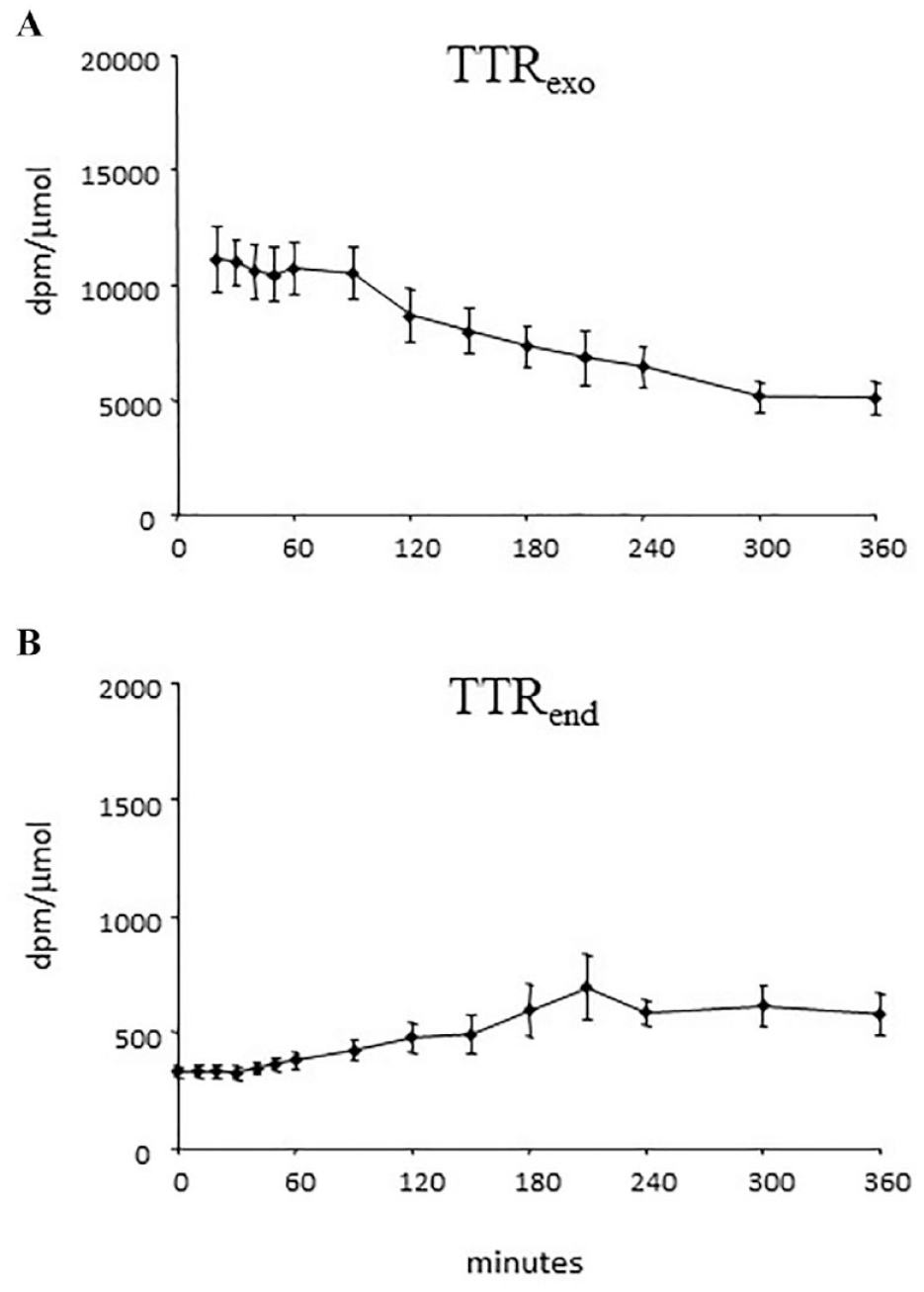
The triple tracer method ⁸⁷ implements the TTR clamp technique to keep the appropriate plasma TTRs constant following glucose ingestion. ¹¹¹ However, instead of infusing labeled glucose at a constant rate, it varies the intravenous infusion rates of 2 different tracers in a manner that mimics the anticipated Ra_meal and EGP (Figure 9, right panel), so that the changes in the plasma TTRs are minimized (Figure 10).

Figure 10.

TTR_exo (in dpm/µmol) (upper) and TTR_end (in dpm/µmol) (lower panel) used in the triple tracer methods in 8 healthy subjects. TTR are in dpm/µmol since in this study the i.v. infused tracer is radioactive. ¹¹⁶ Vertical bars represent standard error (adapted from ¹¹⁶ ).

Briefly, let’s call tracer1 (t₁) the tracer mixed in the meal, with a TTR in the meal equal to TTR_meal, tracer2 (t₂) the tracer infused intravenously to mimic the expected pattern of EGP and tracer3 (t₃) the tracer infused intravenously to mimic the expected pattern of Ra_meal.

Exogenous glucose (G_exo), both labeled and unlabeled, can be derived from t₁ concentration and TTR_meal as reported in equation (31).

Endogenous glucose (G_end) is derived by subtracting exogenous and the i.v. infused tracers concentration (in case both are stable isotopes) from total glucose (G):

$$G_{end}\left(t\right)=G\left(t\right)-G_{exo}\left(t\right)-t_2\left(t\right)-t_3\left(t\right)$$

(37)

Let’s now define 2 TTRs: $TT{R}_{exo}\left(t\right)=\frac{t_3\left(t\right)}{G_{exo}\left(t\right)}$ and $TT{R}_{end}\left(t\right)=\frac{t_2\left(t\right)}{G_{end}\left(t\right)}$ .

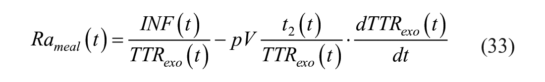
EGP can be derived with equations (34) or (36), while Ra_meal is calculated as:

$$R{a}_{meal}\left(t\right)=\frac{INF\left(t\right)}{TT{R}_{exo}\left(t\right)}-pV\frac{t_3\left(t\right)}{TT{R}_{exo}\left(t\right)}\cdot \frac{dTT{R}_{exo}\left(t\right)}{dt}$$

(38)

or, with Radziuk equation, as:

$$\begin{array}{l}R{a}_{meal}\left(t\right)=\frac{INF\left(t\right)}{TT{R}_{exo}\left(t\right)}-pV\frac{t_3\left(t\right)}{TT{R}_{exo}\left(t\right)}\cdot \frac{dTT{R}_{exo}\left(t\right)}{dt}\\ +k_{21}\left(\frac{q_2\left(t\right)}{TT{R}_{exo}\left(t\right)}-Q_2\left(t\right)\right)\end{array}$$

(38)

It is worth noting that this method requires a priori knowledge of the temporal pattern of change of Ra_meal and EGP. Such knowledge can be relatively easily gained by conducting a few pilot studies and modifying tracer infusion rate (if necessary), so as to minimize the change in plasma TTRs.

The triple tracer method has been presented in, ⁸⁷ and successfully used to assess glucose turnover in elderly vs young subjects and men vs women, ⁴⁰ in untreated ⁶² and treated type 2 diabetes, ³⁶ to assess circadian variation in glucose both in healthy ⁶³ and type 1 diabetes. ⁶⁴ In all these studies, the oral load consisted of a mixed meal (a jello containing dextrose, proteins and fats) labeled with the stable isotope [1- ¹³ C]-glucose and the intravenously infused tracers were the stable isotope [6,6- ² H₂]-glucose and the radioactive [6- ³ H]-glucose. The use of the tritium as third tracer simplified the preelaboration of the data, since specific activity can be directly used instead of TTR in the above equations. However, the use of radioactive tracer is not allowed in children and adolescents, thus, the methodology was successfully implemented in adolescents using 3 stable isotopes ([6,6- ² H₂]-glucose orally administered with an OGTT, [1- ¹³ C]-glucose i.v. infused to mimic Ra_meal and [U- ¹³ C₆]-glucose i.v. infused to mimic EGP). ¹¹⁷

Recently, the triple tracer technique was extended to assess glucose turnover after meals containing complex, instead of simple, carbohydrates. ¹¹⁸ The natural enrichment of [ ¹³ C]polysaccharide in some commercially available grains (eg, Madagascar pink rice and sorghum) was exploited to trace the meal, while [6,6- ² H₂]-glucose and the [6- ³ H]-glucose were intravenously infused in healthy volunteers. As expected, both Ra_meal, EGP and Rd significantly differed between complex and simple carbohydrate containing meals, highlighting that the use of the simple carbohydrate glucose as the carbohydrate source in triple tracer studies may limit the translational applicability of the results since every day’s life meals typically contain complex carbohydrates.

Maximal Models for In Silico Trials: The Uva/Padova Type 1 and the Padova Type 2 Simulators

For reader convenience/information, part of the material reported in this section is taken from ¹¹⁹ and. ¹²⁰

In Silico Clinical Trials (ISCT) are defined as “The use of individualized computer simulation in the development or regulatory evaluation of a medicinal product, medical device, or medical intervention.” ¹¹⁹ The keyword is “individualized.” The idea is to recreate the concept of in vivo trial using an in silico approach, where a large number of individual patients is modeled by initializing a disease/intervention model with quantitative information either measured on an individual (subject-specific model), or sampled from population distributions of those values (population-specific model). As discussed in, ¹¹⁹ realistic ISCTs necessitate the availability of a cohort of in silico subjects spanning the variability observed in the study population, that is, an average model is useless.

After years of rejection, some regulators are now beginning to consider a possible role for computer modeling and simulation in the certification process for biomedical products. The United States Food and Drug Administration (US-FDA) is leading this trend, worldwide. ¹¹⁹

Of course, all this is driven by the growing capability of simulation technologies to accurately simulate complex physiological processes, such as the progression of a disease, the effect of interventions on such progression, and in some cases the manifestation of side effects and complications due to these interventions. This relies on significant pre-competitive research investments done in the last 10 years in the area of physiological modelling. ¹¹⁹

The general approach to establish the credibility of in silico clinical trials revolves around the assumption that in vivo studies, whether on animals or on humans are the most reliable source of information, and any in silico approach should be validated against them. Thus, in the clinical assessment of subject-specific models, a group of patients is examined to collect quantitative information required to initialize the model, which is then used to predict one or more outcome biomarkers for each patient. The same outcome biomarkers are then observed experimentally, whether using an invasive technique or after enough time to make the direct experimental observation possible. ¹¹⁹

All this is based on the assumption that in vivo clinical trials work fine, and the motivation for replacing them is related to the risk, duration or cost that the trial involves, but not to their ability to provide a reliable answer on the safety and/or efficacy of a new biomedical product. ¹¹⁹

In the field of diabetes research, in silico experiments are of enormous value to accelerating technology development since it is often not possible, appropriate, convenient, or desirable to perform an experiment on human subjects because it cannot be done at all, or it is too difficult, too dangerous, or unethical. In such cases, simulation offers an alternative way of experimenting in silico with the system. ¹²⁰ Several simulation models have been published since the 1960s, mostly in biomedical engineering journals^121-127 but their impact in the field has been virtually zero. The reason is that all of these models were average models, and, as a result, their capabilities were generally limited to predicting a population average that would be observed during a clinical trial. However, given the large inter-individual variability, an average model approach cannot describe realistically the variety of individual responses to diabetes treatment. Thus, to enable realistic in silico experimentation, it is necessary to have a diabetes simulator equipped with a cohort of in silico subjects that spans sufficiently well the observed inter-individual variability of key metabolic parameters in the population of people with type 1 (T1D) and type 2 (T2D) diabetes.

In particular, in T1D, in silico experiments have been of enormous value to accelerate technology development, for example, subcutaneous glucose sensors, novel insulin molecules and the artificial pancreas, thanks to the availability of the U.S. Food and Drug Administration (FDA) accepted UVA/Padova T1D simulator,^128-130 which allows a time- and cost-effective alternative to preclinical studies, (eg, ¹³¹ )

The FDA Accepted UVA/Padova T1D Simulator

The FDA-accepted University of Virginia (UVA)/Padova T1D simulator has had a serendipity beginning. In 2006, as part of a NIH program project studying the effects of 2-year administration of youth pills in elderly men and women, physiological performance, body composition, and bone density were measured in 204 individuals without diabetes.^40-119 These subjects underwent a triple-tracer meal protocol (see section 7.2.2) which provided, in addition to plasma glucose and insulin concentrations, model-independent estimates of key fluxes of the glucose system, including the rate of appearance in plasma of ingested carbohydrates, endogenous glucose production, glucose utilization, and insulin secretion.^40-120 This rich flux and concentration portrait was key to develop a large-scale glucose–insulin model, which was impossible to build from only plasma glucose and insulin concentrations. A model including 18 differential equations with 42 parameters, 33 of which were free and 9 were derived from steady state constraints, was identified in each individual using a Bayesian forcing function strategy. ¹³² From the model parameter estimates of the 204 subjects participating in this study, the inter-individual variability was described in a population without diabetes. From there, using the joint multivariate probability distribution of the model parameters, any number of virtual subjects could be generated by random sampling, thereby producing a virtual population. Simultaneously with the events above, and thanks to the advent of minimally invasive subcutaneous (sc) continuous glucose monitoring (CGM), increasing academic, industrial, and political effort has been focused on the development of a sc–sc closed-loop control system for diabetes, which is known as the artificial pancreas (AP). Generally, the AP uses a CGM coupled with a sc insulin infusion pump and a control algorithm directing insulin dosing in real time.

In September 2006, the Juvenile Diabetes Research Foundation (JDRF), initiated the Artificial Pancreas (AP) Project and funded a consortium of university centres in the United States and Europe to carry closed-loop control research. At the time, the regulatory agencies mandated demonstration of the safety and feasibility of AP systems in animals, for example, dogs or pigs, before any testing could begin in humans. This approach is well illustrated by 2 papers showing the use of the Medtronic AP system first in 8 dogs ¹³³ and then, later, in 10 people with T1D. ¹³⁴ However, it also became evident that animal studies were slow, not powered for variability and costly, and that a simulator of T1D would allow a cost-effective pre-clinical testing of AP control strategies by providing direction for subsequent clinical research and ruling out ineffective control scenarios. We argued that a reliable large-scale simulator would account better for inter-subject variability than small-size animal trials and would allow for fast and extensive testing of the limits and robustness of AP control algorithms.

We therefore set to build a simulation environment based on the data and the expertise accumulated at the University of Padova and the University of Virginia, 2 groups that were already collaborating on several aspects of diabetes technology. A first necessary modification of the existing model ¹³² was the substitution of endogenous insulin secretion subsystem with an exogenous sc insulin delivery, that is, an insulin pump. This required describing insulin absorption with a 2-compartment model approximating non-monomeric and monomeric insulin fractions in the sc space. Given the absence in 2006 of tracer studies in T1D similar to those described above for healthy subjects, a more difficult task was the description of inter-person variability.

In order to obtain the joint model parameter distributions in T1D, we introduced certain clinically relevant modifications to the models developed in health. The resulting T1D simulation model included 13 differential equations and 35 parameters, 26 of which were free and 9 were derived from steady-state constraints. Once the T1D model was built, its validity was tested using number of T1D data sets including adults, adolescents, and children. Now the UVA/Padova simulator is equipped with 300 virtual subjects: 100 adults, 100 adolescents, and 100 children, spanning the variability of the T1D population observed in vivo. In addition, the simulator is equipped with models of CGM and insulin pumps. With this technology, any meal and insulin delivery scenario can be tested efficiently in silico, prior to its clinical application. ¹²⁸ After extensive testing, in January 2008, this simulator was accepted by the US FDA as a substitute to animal trials for the pre-clinical testing of control strategies in AP studies and has been adopted by the JDRF AP Consortium as a primary test bed for new closed-loop control algorithms. The simulator was immediately put to its intended use with the in silico testing of a new model predictive control (MPC) algorithm, and in April 2008, an investigational device exemption (IDE) was granted by the FDA for a closed-loop control clinical trial. This IDE was issued solely on the basis of in silico testing of the safety and efficacy of AP control algorithm, an event that set a precedent for future clinical studies. ¹³¹ In brief, to test the validity of the computer simulation environment independently from the data used for its development, a number of experiments were conducted, aiming to assess the model capability to reflect the variety of clinical situations as closely as possible. These experiments included the following:

1. Reproducing the distribution of insulin correction factors in the T1D population of children and adults, which tests that the variability in the action of insulin administered by control algorithms will reflect the variability in observed insulin action;

2. Reproducing glucose traces in children with T1D observed in clinical trials performed by the Diabetes Research in Children Network (DirecNet) consortium;

3. Reproducing glucose traces of induced moderate hypoglycemia observed in adults in clinical trials at the UVA, which provides comprehensive evaluation of control algorithms during hypoglycemia.

Thus, the following paradigm has emerged: (1) in silico modeling could produce credible preclinical results that could substitute certain animal trials and (2) in silico testing yields these results in a fraction of the time and the cost required for animal trials. This was a paradigm change in the field of T1D research: for the first time, a computer model has been accepted by a regulatory agency as a substitute of animal trials in the testing of insulin treatments. Since its introduction, this simulator enabled an important acceleration of AP studies, with a number of regulatory approvals obtained using in silico testing. However, one needs to emphasize that good in silico performance of a control algorithm does not guarantee in vivo performance; it only helps to test the stability of the algorithm in extreme situations and to rule out inefficient scenarios. Thus, computer simulation is only a prerequisite to, but not a substitute for, clinical trials.

Later, new data became available on hypoglycemia and counter-regulation, which allowed an update of the in silico model in 2014. ¹²⁹ This new version has been proven to be valid on single-meal scenarios showing that the simulator was capable of well describing glucose variability observed in 24 type 1 diabetes subjects who received dinner and breakfast in 2 occasions (open- and closed-loop), for a total of 96 post-prandial glucose profiles. ¹³⁵ The simulator domain of validity was then extended by the introduction of diurnal patterns of insulin sensitivity based on data in 19 T1D subjects who underwent a triple-tracer study^64-136 (see paragraph 3.4). This has allowed the incorporation of a circadian time-varying insulin sensitivity into the simulator, thus making this technology suitable for running one-day multiple-meal scenarios and enabling a more robust design of AP control algorithms. ¹³⁰

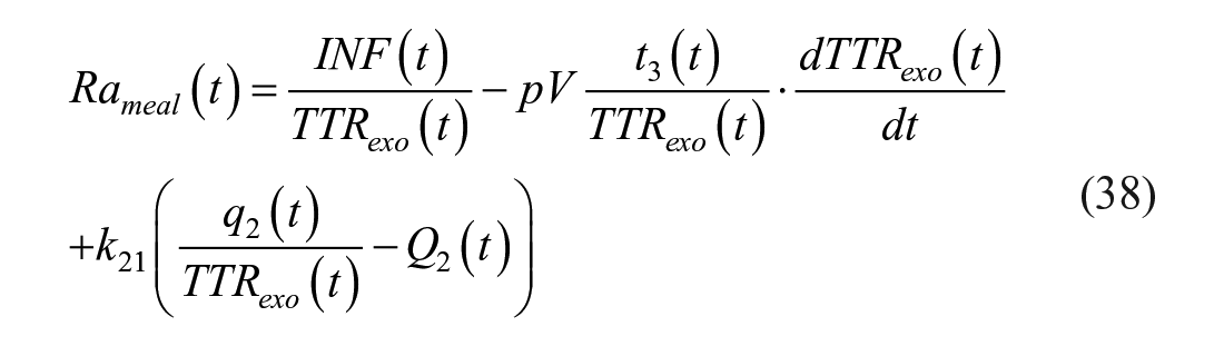
Finally, another validation of the simulator was done by comparing its predictions to data of 47 T1D subjects from 6 clinical centres, who underwent 3 randomized 23-h admissions, one open- and 2 closed-loop. The protocol approximated real life with breakfast, lunch and dinner and collected 141 daily traces of glucose and insulin concentrations. We used Maximum a Posteriori Bayesian approach, which exploited both the information provided by the data and the a priori knowledge on model parameters represented by the joint parameter distribution of the simulator. Plasma insulin concentration was used as model-forcing function, that is, assumed to be known without error. The identification of the simulator on a specific person provided an in silico “clone” of this person; thus, the possibility emerged to clone a large number of T1D individuals and to move from single-meal to breakfast/lunch/dinner scenario, thus accounting for intra-subject variation in glucose absorption and insulin sensitivity. ¹³⁷ This new feature, together with a model of dawn phenomenon data has been incorporated in a new version of T1D simulator. ¹³⁰ This version also includes a more realistic model of sc insulin delivery, models of both intra-dermal and inhaled insulin pharmacokinetics, and new models of error affecting continuous glucose monitoring and self-monitoring of blood glucose devices (Figures 11 and 12).

Figure 11.

Scheme of latest version of the UVa/Padova T1D simulator, incorporating time-varying parameters describing intraday variability of insulin sensitivity and dawn phenomenon. The simulator also includes various insulin delivery routes (subcutaneous fast-acting insulin, intradermal and inhaled insulins) and glucose monitoring devices (both CGM and SMBG) (adapted from ¹³⁰ ).

Figure 12.

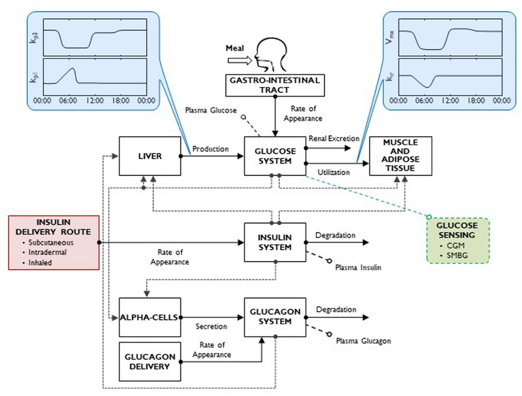
Simulated plasma glucose (upper) and insulin (lower panels) in the 100 in silico adults (left), adolescents (middle), and children (right panels) available in the UVa/Padova T1D simulator. Subjects underwent a 24-hour scenario with 3 identical meals (60 g of CHO) at 7:00 am, 1:00 pm, 7:00 pm, respectively, and received optimal subcutaneous insulin basal and bolus (adapted from ¹³⁰ ).

Since 2012, the AP studies successfully moved to outpatient free-living environment and became longer, with durations of up to several weeks/months.^138-143 These trials are collecting large amounts of data, typically including closed-loop control and an open-loop mode as a comparator.

The UVA/Padova T1D simulator has been used in a variety of contexts by several research groups in academia, by companies active in the field of diabetes pharma and technology and has led to more than one thousand publications in peer reviewed journals. Three major application areas which emerged recently are:

• i) new generation of closed-loop control algorithms. In particular, the simulator allows to assess individualization strategies, that is, methods for tuning the control algorithm to a specific person ¹⁴⁴ and, thus making the AP to be adaptive, that is, learning from the behaviour in time of a specific person.^145-149

• ii) testing safety and efficacy of a Do-It-Yourself algorithm, specifically an AndroidAPS implementation of the OpenAPS algorithm. ¹⁵⁰

• iii) detection of insulin pump malfunctioning to improve safety of an artificial pancreas. ¹⁵¹

• iv) testing of new insulin molecules (Figure 13), for example, pramlintide,^152,153 inhaled technosphere insulin, ¹⁵⁴ fast ¹⁵⁵ and long acting insulin analogues.^156,157

• v) testing glucose sensors. Of particular relevance was the use of the simulator to address an important topic of investigation for the diabetes community and regulatory agencies: is CGM safe and effective enough to substitute SMBG in diabetes management? In silico clinical trials were performed with a patient decision-making model ( ¹⁵⁸ ) able to recreate real-life conditions (eg, 100 adults and 100 pediatric patients, 3 meals per day with variability in time and amount, and meal bolus behaviour) (Figure 14).

Figure 13.

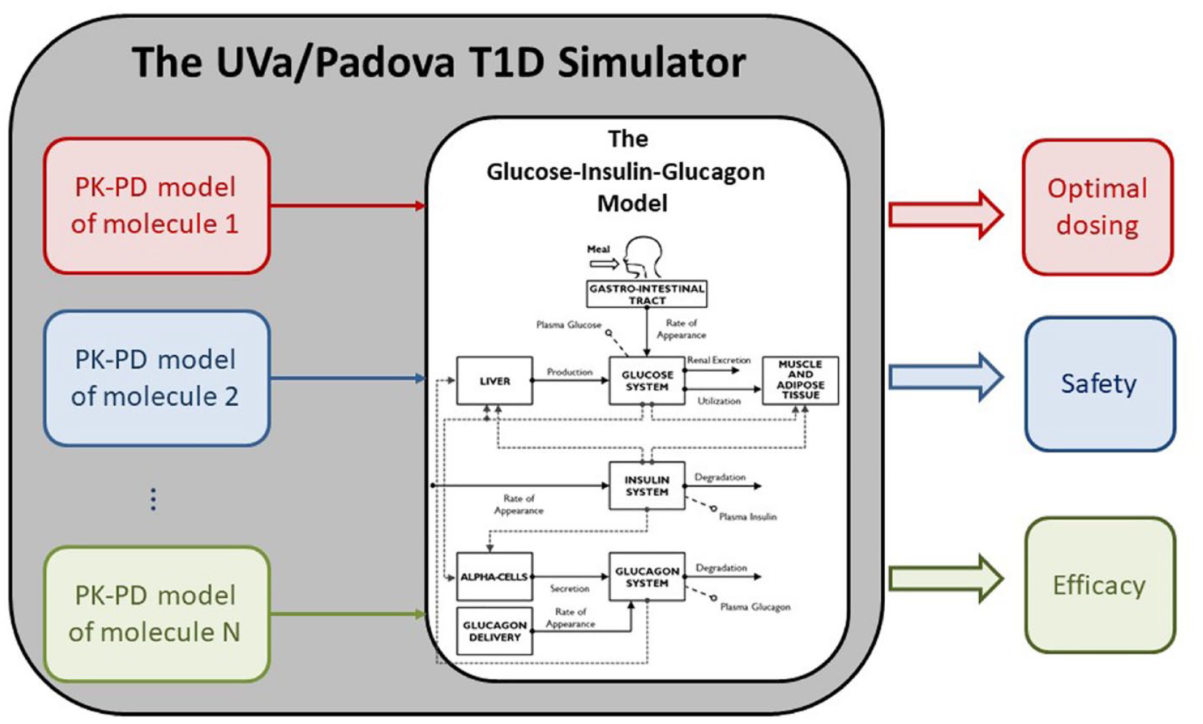
The use of the UVa/Padova T1D simulator for testing new molecules: once the PK-PD of the molecule under investigation is incorporated in the simulator, simulations can be run predicting clinical outcomes, for example, optimal dosing, safety and efficacy.

Figure 14.

Block-scheme representing the T1D patient decision simulator. Arrows entering each block are inputs, while arrows exiting are causally-related outputs. The input of the simulator is the sequence of meals, while the output is the BG concentration profile. The simulator includes parameters describing the patient’s physiology and therapy. The picture reports representative time courses for meals in input and BG in output for a simple scenario in which the patient takes 50 g for breakfast at 07:00 am (adapted from ¹⁵⁸ ).

The simulations helped the outcome of an FDA panel meeting.^159,160

The Padova T2D Simulator

Among the almost 500 million people in the world having diabetes, only 10-15% has T1D. The vast majority are subjects with type 2 diabetes (T2D). These patients are often treated with medications to control their blood glucose levels: some of these medications are orally administered (eg, biguanides, sulfonylureas, Dipeptidyl Peptidase 4 inhibitors) ¹⁶¹ some others are given by injection (eg, insulin, amylin analogues, Glucagon-Like Peptide-1 receptor agonists). ¹⁶² Testing new treatments or combination of medications is time consuming and expensive. Therefore, a simulator to perform ISCT in T2D would be highly desirable. Very recently, we have developed a single meal T2D simulator ¹⁶³ using a data base of 51 T2D subjects,^36,60,62,164 studied with the triple-tracer meal technique ⁴⁰ and following the successful modeling methodology employed in the development of the T1D simulator.

Figure 15.A reports the mean ± standard deviation (SD) of measured plasma glucose, insulin and C-peptide concentrations, Ra_meal, EGP and U in T2D subjects. The model scheme describing the glucose-insulin interaction in T2D subjects is shown in Figure 15.B (we refer to ¹⁶³ for the complete list of model equations and the meaning of the model parameters).

Figure 15.

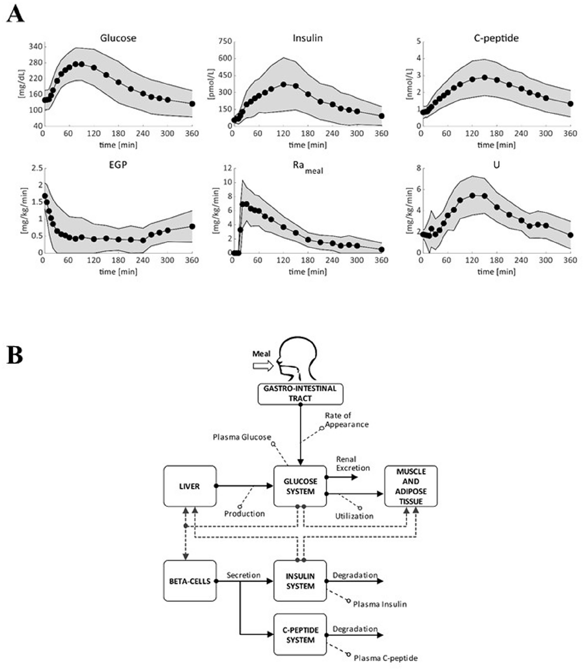
Upper panel: average (filled circle) ± standard deviation (SD, shaded area) plasma glucose, insulin and C-peptide concentration and estimated endogenous glucose production (EGP), glucose rate of appearance (Ra_meal) and glucose utilization (U) in T2D subjects (N = 51). Lower panel: scheme of the T2D simulation model. Metabolic fluxes are indicated with continuous lines, while control actions are represented by dashed lines. Adapted from. ¹⁶³

Briefly, the model derives from that proposed by Dalla Man et al. ¹³² Like the original model, this one describes the glucose transit through the gastro-intestinal tract, the action of insulin on glucose utilization and endogenous production, and the control of glucose on insulin secretion. The glucose subsystem is described by a 2-compartment model: ¹³² insulin-independent utilization occurs in the first compartment, representing plasma and rapidly equilibrating tissues, while insulin-dependent utilization occurs in a remote compartment, representing peripheral tissues. At variance with, ¹³² a 3-compartment model is used to describe insulin kinetics in the liver (Il), in the plasma (I_p), and in extravascular space (I_ev).^165,166 A 2-compartment model is also added to describe C-peptide kinetics.^23,25

Metabolic fluxes accounted in the model are EGP, Ra_meal, glucose utilization (U), β-cell insulin secretion rate (ISR), and hepatic insulin extraction (HE). EGP suppression is assumed to be linearly dependent on plasma glucose, liver insulin, and a delayed plasma insulin signal; ⁸⁸ one of the key model parameters is hepatic insulin sensitivity (k_p3), which quantifies insulin control on EGP suppression. Ra_meal is described with a 3 compartment model, 2 representing the stomach (solid and triturated compartments), and one the gut. ¹⁶⁷ Glucose utilization, U, is made up of 2 components: insulin-independent utilization (Uii) in the brain and erythrocytes is assumed constant, while insulin-dependent utilization (U_id) in muscle and adipose tissues depends nonlinearly (Michaelis–Menten) from glucose in the tissues; ¹⁶⁸ one of the key model parameters is disposal insulin sensitivity (V_mx). The model also assumes that, when glucose decreases below its basal value, a paradoxical increase in insulin sensitivity occurs, as previously described. ¹²⁹ ISR is assumed to be made of a basal, a dynamic and a static component, and modeled as in, ⁴⁸ HE is assumed to be linearly related to plasma glucose concentration as in. ¹⁶⁶

The availability of the glucose fluxes in addition to plasma glucose, insulin and C-peptide concentrations, allowed identifying the model by using a system decomposition and forcing function strategy, paralleling what was done in. ¹³² The parameter estimates, obtained from model identification in the 51 T2D subjects, were used to build up the joint parameter distribution, which allowed to generate a T2D in silico population.

The model well predicted glucose, insulin, C-peptide, EGP, Ra_meal and U data of T2D subjects and the distributions of some key parameters in T2D vs healthy subjects (H) are reported in. ¹⁶³

A population of 100 in silico T2D subjects was generated. Simulated plasma glucose, insulin and C-peptide are compared with T2D data. ¹⁶³ Results show a good agreement between simulations and data both in terms of population median and variability.

An interesting peculiarity of the simulator, besides well covering the average dynamics, lies in the possibility to evaluate the efficacy of a given treatment in rare, but not so rare, subjects, as discussed in a case study in. ¹⁶³

This new T2D simulator has the potential to accelerate the research needed to put on the market new antidiabetic drugs. By allowing the evaluation of many treatment scenarios in a cost-effective way.

The availability of 100 virtual subjects is important, since it allows running in silico large-scale trials, as usually occurs in phase II clinical trials. In addition, since virtual subjects can undergo the identical experimental scenario several times, one can implement an ideal crossover design, where physiological intra-subject variability is minimized (and controlled by the investigator).

Furthermore, the possibility to virtually recruit a subset of subjects with common characteristics, as shown in the case study of ¹⁶³ permits to extensively study situations characterized by extreme parameter vectors, sampled from the distribution tails. This could possibly be used for optimizing diabetes therapy also in such rare pathological conditions.

The domain of validity of the simulator is currently the single meal scenario. This might be a limitation for testing treatments that might have a different effect depending on time of administration. For example, long-acting insulin analogues might lead to a different glucose profile depending on morning or evening dosing, as already observed in T1D. ¹⁶⁹ A future model refinement will include the description of intra-/inter-day variability of key model parameters, similarly to what has been recently done in H and T1D,^63,64 thus improving the simulator reliability on long-term scenarios. In this regard, an ongoing study in T2D will provide important insights on intra- and inter-day variability of insulin sensitivity and beta-cell function.

Conclusions

In this paper we have accompanied the reader to our model-based understanding of the glucose system. We have started with a concise historical background to put our story in a proper perspective. Focus has been on minimal models and maximal models.

Minimal models provide parametric portraits of the glucose-insulin system from a physiological test, either an MTT or and OGTT. In some sense, minimal models allow to implement Galileo Galilei’s statement while teaching at our University in 1592-1610 “. . .measure what is measurable and make measurable what is not. . .”.The key role of tracers to arrive at a more detailed whole-body picture of insulin action by segregating disposal and liver insulin sensitivity has been discussed. Powerful multi-tracer techniques, that is, the multiple tracer dilution and the positron emission tomography, which allow to arrive at a more intimate picture insulin action on skeletal muscle has been emphasized. Finally, multi-scale modeling aiming to effectively capture biological interdependencies and interactions among multiple scales has been discussed for insulin secretion by relation whole-body indices to cellular secretory parameters.

Maximal models allow to perform in silico studies in life sciences and clinical trials, following their successful but easier use in physical and engineering sciences. Tracers have also allowed to move from a parametric to a flux portrait, enabling the quantitative assessment of postprandial glucose metabolism, and de facto allowing to put large scale simulation of Type 1 and Type 2 diabetes on solid data-bases. The FDA accepted UVA/Padova Type 1 simulator was an unprecedented event in the biological modeling community and proved to be a very useful tool to safely and effectively test in silico artificial pancreas control algorithm, glucose sensors for non-adjunctive use and new insulin molecules.