Sage Journals: Discover world-class research

Abstract

Background:

In type 1 diabetes (T1D) research, in-silico clinical trials (ISCTs) have proven effective in accelerating the development of new therapies. However, published simulators lack a realistic description of some aspects of patient lifestyle which can remarkably affect glucose control. In this paper, we develop a mathematical description of meal carbohydrates (CHO) amount and timing, with the aim to improve the meal generation module in the T1D Patient Decision Simulator (T1D-PDS) published in Vettoretti et al.

Methods:

Data of 32 T1D subjects under free-living conditions for 4874 days were used. Univariate probability density function (PDF) parametric models with different candidate shapes were fitted, individually, against sample distributions of: CHO amounts of breakfast (CHO_B), lunch (CHO_L), dinner (CHO_D), and snack (CHO_S); breakfast timing (T_B); and time between breakfast-lunch (T_BL) and between lunch-dinner (T_LD). Furthermore, a support vector machine (SVM) classifier was developed to predict the occurrence of a snack in future fixed-length time windows. Once embedded inside the T1D-PDS, an ISCT was performed.

Results:

Resulting PDF models were: gamma (CHO_B, CHO_S), lognormal (CHO_L, T_B), loglogistic (CHO_D), and generalized-extreme-values (T_BL, T_LD). The SVM showed a classification accuracy of 0.8 over the test set. The distributions of simulated meal data were not statistically different from the distributions of the real data used to develop the models (α = 0.05).

Conclusions:

The models of meal amount and timing variability developed are suitable for describing real data. Their inclusion in modules that describe patient behavior in the T1D-PDS can permit investigators to perform more realistic, reliable, and insightful ISCTs.

Keywords

in-silico clinical trials maximum absolute difference parametric modelling machine learning support vector machine

Introduction

In the past 15 years of type 1 diabetes (T1D) research, in-silico clinical trials (ISCTs), performed using simulators relying on mathematical models of glucose-insulin system dynamics, have accelerated the development of new treatments^1-4 and drugs,^5-7 and have facilitated the design of clinical studies.^8-11 ISCTs allow investigators to carry out a vast number of experiments quickly, in order to evaluate, for example, new algorithms in high-risk scenarios, and so offer considerable economic and human resource savings.^12-14 In order to perform ISCTs, mathematical models mimicking the physiology and, often, also the lifestyle of T1D patients, are required.

While a number of simulation tools effectively tackling various aspects of T1D pathophysiology^15-18 have been described in the literature, the mathematical description of aspects mainly related to patient behavior has, so far, been rarely investigated.¹⁹ Nonetheless, lifestyle can remarkably affect the quality of glucose control in T1D management. A first attempt to take these aspects into account in a simulator, and to enable more realistic ISCTs, was the T1D Patient Decision Simulator (T1D-PDS) proposed by Vettoretti et al.²⁰ Over the state-of-the-art UVa/Padova model of glucose, insulin, and glucagon kinetics,¹⁵ the T1D-PDS mounted additional modules describing the accuracy of glucose monitoring devices, pump insulin administration, and (of special interest in this paper) some behaviors of patients when making treatment decisions. Specifically, the T1D-PDS embeds models describing the variability in meal time and amount, behavior in tuning hypotreatment consumptions and insulin correction bolus injections, and the errors in meal bolus time and in carbohydrates (CHO) counting. Though the T1D-PDS was seen as useful for augmenting the credibility of ISCTs,^21,22 its module describing meal variability did leave some room for improvement. In fact, breakfast, lunch, and dinner CHO amounts are described by uniform distributions, mealtimes are considered uncorrelated to each other, and there is no model of snacks.

In this work, we aim to overcome these limitations by developing new mathematical models mimicking the meal amount and timing variability in individuals with T1D under free-living conditions. Specifically, by leveraging a published dataset of 32 subjects—for a total of 4874 days and 17 111 meals—we derive a new model for the three main meals, ie, breakfast, lunch, and dinner, which considers the CHO amount of each meal and the time between consecutive meals. We also develop a model for the CHO amount of snack and a model to realistically simulate snack timing, taking into account a group of variables that influence the likelihood of consuming a snack during the day. Lastly, we embed the new models into the T1D-PDS and we compare the resulting simulations against real data.

Methods

Dataset

Data were collected in a multinational, randomized, crossover trial made for the AP@home EU project.²³ The study involved 32 individuals with T1D, recruited from three medical centers: Padova (Italy), Montpellier (France), and Amsterdam (Netherlands). Participants were 44% women, and 47.0 ± 11.2 years old, with mean diabetes duration of 28.6 ± 10.8 years, HbA1c of 8.2 ± 0.6% (65.9 ± 4.8 mmol/mol), and BMI of 25.1 ± 3.5 kg/m². The study aimed to compare the artificial pancreas (AP) and the sensor augmented pump (SAP) therapy, by assessing their impact on glucose control. Subjects were randomly assigned to two months of AP, from dinner to waking up, plus SAP therapy during the day, versus two months of SAP use only. A subgroup of 20 subjects was monitored in a further one month trial under all-day AP therapy.²⁴ Then, 18 out of the previous 20 subjects underwent a last one month follow-up with a personalized all-day AP.²⁵

During AP therapy, participants used the DiAs platform²⁶ to promptly register many variables, such as meal CHO content, insulin bolus administration, and hypotreatments. In particular, to perform an insulin bolus in occasion of a meal, it was mandatory for trial participants to insert in the platform their CHO amount. Hypotreatments were recorded separately from other meals. During SAP therapy, participants were encouraged to report any items of possibly useful information (eg, time and CHO amount of meal intakes and insulin boluses) in a handwritten diary.

Since we aimed to model the behavioral aspects of people with diabetes, independent of their therapy, we considered data collected under SAP therapy and AP therapy as a single dataset, thus obtaining a total of 17 111 meals collected over 4874 days.

Data Pre-Processing

We looked for consecutive meals registered temporally close to each other, since they could very likely be parts of the same main meal—hereafter referred to as “fragmented” meal. For example, a “fragmented” meal could be a lunch, in which the main course and the dessert were reported separately as two sub-meals. Specifically, the meals that were no more than 25 minutes distant from one another were considered as part of the same “fragmented” meal. Thus, the sub-meals of each “fragmented” meal were assembled into a single meal by setting the total meal amount to the sum of the sub-meals CHO amounts, and the mealtime to the time of the earliest sub-meal. With this criterion, 2.49% of all the registered meals were detected as sub-meals. A robustness analysis over the temporal threshold to identify sub-meals (here fixed at 25 minutes) showed that increasing this value, just minimally affected the number of detected “fragmented” meals.

In order to model breakfast, lunch, dinner, and snack separately, all meal data were labeled. Although in real life not all the meals fall under these meal categories (eg, a brunch can be difficult to classify), having an exact meal labeling is not crucial for our final purpose of improving the meal generation module in the T1D-PDS. Indeed, to reliably model meal amount and timing variability, what really matters is to allocate the CHO intakes over the hours of the day in a plausible way, which reflects what is observed on real data.

To label the main meals (ie, breakfast, lunch, and dinner), we selected meal-specific time windows as follows: 4:00 AM-11:30 AM for breakfast, 11:35 AM-4:30 PM for lunch, 4:35 PM-3:55 AM for dinner.²⁷ Main meals were identified as being those with the biggest CHO amount amongst all the meal intakes registered inside each window. The remaining meal data could be related either to hypotreatments or to snacks. In the AP scenario, the DiAs platform forced users to record hypotreatments separately from other meal intakes; thus, the related data were already labeled. Therefore, once the main meals had been identified, the remaining CHO intakes were presumed to be snacks. In the SAP scenario, once the main meals had been identified, since a further classification between hypotreatments and snack would have added uncertainty over the data, the other CHO intakes were not labeled, and thus, were not assigned to a specific CHO intake category, ie, they were excluded from the analysis.

Note that meal data registered on handwritten diaries (ie, those collected in SAP therapy) were manually analyzed and meals likely to be inaccurately reported (eg, a slight number of meals not associated to an insulin bolus) were discarded.

The pre-processing step provided 11 460 main meals (3643 breakfasts, 3837 lunches, 3980 dinners) and 1218 snacks. These data were used to derive models of meal CHO amounts and main meal timing, as well as a model of the probability of consuming a snack in different moments of the day.

A sensitivity analysis to evaluate the impact of mislabeling over the models of meal amount and timing is reported in the Appendix.

Meal Carbohydrates Content and Main Meal Time Variability Models

The statistical distributions of the CHO content of breakfast, lunch, dinner, and snack were modeled by parametric probability density function (PDF) models. To describe main meal timing by taking into account the correlation between consecutive meals, a parametric PDF model was also derived for breakfast time, time between breakfast-lunch, and time between lunch-dinner. In total, seven variables describing meal amounts and times were modeled. For each variable, we considered the following 10 candidate univariate PDF models: Gaussian, lognormal, loglogistic, gamma, generalized-extreme-value (GEV), t-Student, exponential, inverse Gaussian, logistic, and uniform, whose equations are reported in the second column of Table 1. The model providing the best description of the data was selected for each variable as follows.

Table 1.

Candidate PDF Model Equations.

Candidate PDF model	Equation
Gaussian	$F (x; μ, σ) = \frac{1}{σ \sqrt{2 π}} \exp (- \frac{1}{2} {(\frac{x - μ}{σ})}^{2})$
Lognormal	$F (x; μ, σ) = \frac{\exp (- \frac{{(\ln x - μ)}^{2}}{2 σ^{2}})}{x \sqrt{2 π} σ}$
Loglogistic	$F (x; α, β) = \frac{1}{α} \frac{1}{x} \frac{\exp (\frac{\log (x) - β}{α})}{{(1 + \exp (\frac{\log (x) - β}{α}))}^{2}}$
Gamma	$F (x; α, λ) = \frac{x^{α - 1} e^{- \frac{x}{λ}}}{λ^{α} Γ (α)}$
GEV	$\begin{array}{l} F (x; μ, σ, ξ) = \frac{1}{σ} e x p \\ {- {[1 + ξ (\frac{x - μ}{σ})]}^{- \frac{1}{ξ}}} {[1 + ξ (\frac{x - μ}{σ})]}^{- 1 - \frac{1}{ξ}} \end{array}$
t-Student*	$F (x; ν) = \frac{Γ (\frac{ν + 1}{2})}{\sqrt{ν π} Γ (\frac{ν}{2})} {(1 + \frac{x^{2}}{ν})}^{- \frac{ν + 1}{2}}$
Exponential	$F (x; λ) = λ e^{- λ x}$
Inverse Gaussian	$F (x; μ, λ) = \sqrt{\frac{λ}{2 π x^{3}}} \exp [- \frac{λ {(x - μ)}^{2}}{2 μ^{2} x}]$
Logistic	$F (x; μ, s) = \frac{\exp (- \frac{x - μ}{s})}{s {(1 + \exp (- \frac{x - μ}{s}))}^{2}}$
Uniform	$F (x; a, b) = \frac{1}{b - a}, f o r a \leq x \leq b$

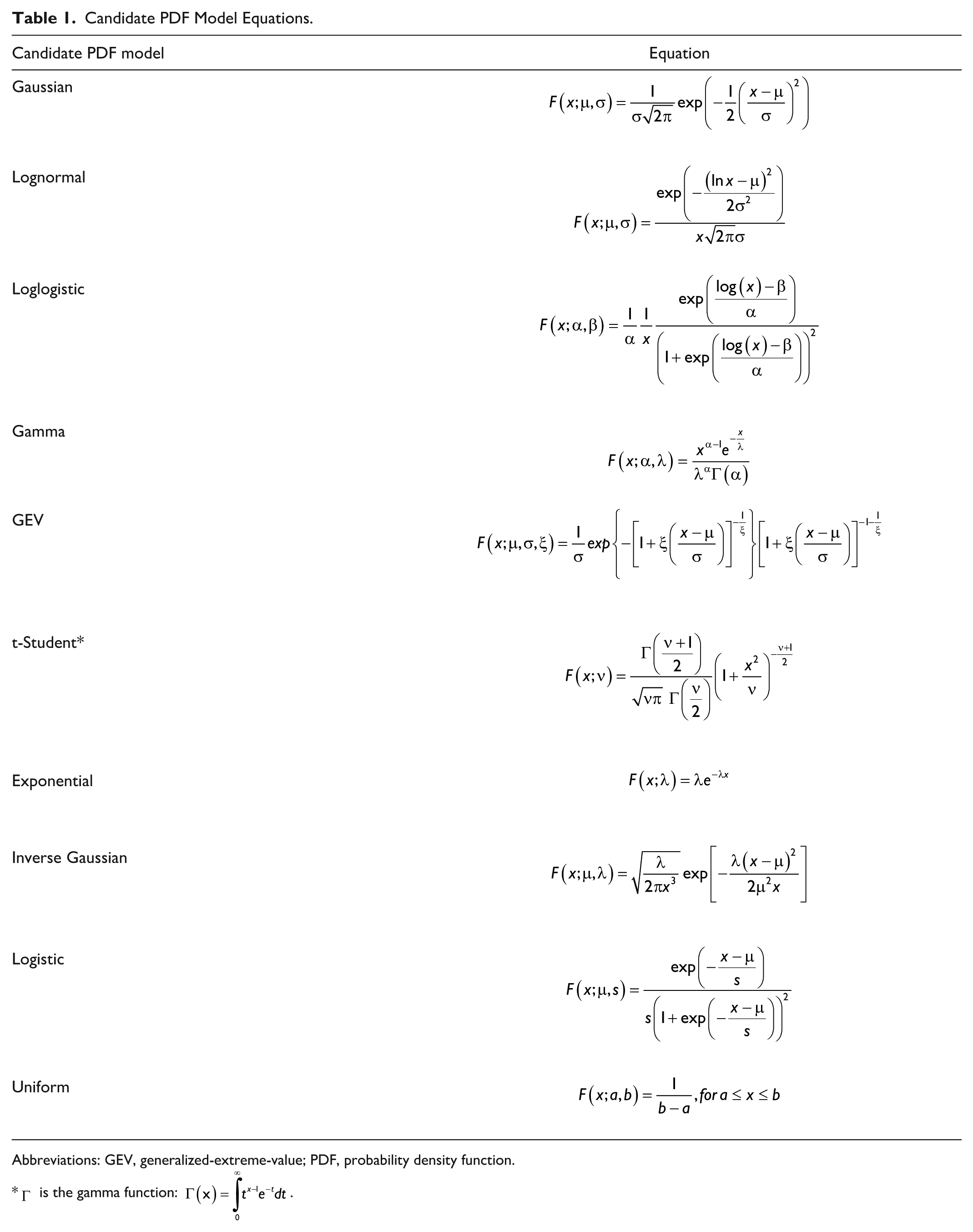
Abbreviations: GEV, generalized-extreme-value; PDF, probability density function.

$Γ$ is the gamma function: $Γ (x) = \int_{0}^{\infty} t^{x - 1} e^{- t} d t$ .

For each variable of interest, we randomly split the available data into training set (TR) and test set (TE), whose cardinalities were, respectively, 70% and 30% of the entire dataset. TR data were used to fit the 10 candidate PDF models, whose parameters were estimated by maximum likelihood (ML). Then, a random sample was extracted by each of the PDF models identified and compared to the TE through computation of a measure of distance between the empirical distribution functions (EDFs) of the two samples.^28-30 The EDF is a discrete estimate of the cumulative distribution function of a random variable, obtained by assigning equal probability to each observation in a sample. As reported in Eq. (1), we computed the maximum absolute difference (MAD, also known as the Kolmogorov-Smirnov statistic) between the EDF of the TE data ( $\hat{F} (x)$ ) and the EDF of the sample generated by the i-th hypothesized PDF model (ie, $G_{i} (x)$ ).

M A D_{i} = \max_{x} (| \hat{F} (x) - G_{i} (x) |)

(1)

To reduce the sensitivity to the TR-TE split, the procedure was re-iterated for 100 different TR-TE splits. Then, the median [25th-75th percentiles] MAD for each candidate PDF model were extracted. Lastly, the PDF model providing the lowest median MAD was selected as the most suitable model and its parameters are re-estimated on the entire dataset.

To visually check the fit quality, the obtained PDF models were compared to the normalized histograms of all the data used to fit the models. In addition, a quantile-quantile plot of the entire dataset and the selected PDF model was reported for each variable. Then, 100 random samples of the same size as the numerosity of available data for each variable of interest were extracted by the final PDF models and their EDFs compared to the EDF of the whole dataset.

Snack Time Variability Model

While main meals are usually consumed three times per day inside time windows sufficiently consistent between individuals,²⁷ snack time clearly has much more inter- and intra-subject variability. The number of snacks consumed per day, and the time windows in which a snack is consumed, can be heavily dependent both on a subject’s habits and on daily conditions (eg, previous meal sizes and times). To obtain a plausible model for describing T1D patient behavior when consuming snacks, we looked for variables that could influence snack consumption times in the dataset being analyzed. To do this, we derived a support vector machine (SVM) classifier able to predict the occurrence of a snack in fixed time windows, based on predictors collected back in time.

The dataset to derive the model was built as follows. We split each subject’s trial into contiguous three-hour observation windows and labeled them with “1,” if at least one snack was consumed inside the window, or “0” otherwise. The total number of windows was 8405: 1028 observations labeled as “1,” and 7377 labeled as “0.”

Then, for each three-hour window, possible predictors of the label were extracted, either from portions of the trial before the observation window, or from the patient’s demographic data. We considered the following 13 features: (i) subject’s age; (ii) body weight (BW); (iii) CHO amount of the last meal intake before the observation window; (iv) the time from that meal; (v) sum of the CHO amount consumed in the last one hour, (vi) four hours, and (vii) six hours before the observation window; (viii) mean continuous glucose monitoring (CGM) in the previous one hour, (ix) four hours, and (x) six hours before the observation window; (xi) first CGM value of the observation window; (xii) CGM rate-of-change in the one hour before the observation window; (xiii) time of the observation window (categorical variable equal to 1, 2, 3, 4 if the first sample in the window is in the interval 5:00 AM-10:55 AM, 11:00 AM-4:55 PM, 5:00 PM-10:55 PM, 11:00 PM-4:55 AM, respectively).

The final dataset was randomly divided into TR (cardinality: 80%) and TE (cardinality: 20%), maintaining the same proportion of the labels: 5902 (87.78%) “0,” 822 (12.22%) “1” in the TR and 1475 (87.75%) “0,” 206 (12.25%) “1” in the TE. A z-score standardization was performed on the features using their mean and their standard deviation in the TR.³¹

As classifier, we used a nonlinear SVM with a radial basis function (RBF) kernel. Using RBF kernels is a widely adopted strategy used to map the inputs into a high-dimensional feature space in a flexible way, in order to make the SVM more robust for any kind of data to achieve a highly accurate classification rate.^32,33 Moreover, being the dataset unbalanced, with the number of “0” greater the number of “1,” two different weights for the two classes were used during the training, according to the following rule of thumb:

$w_{i} = \frac{N}{K n_{k}}$

Where $N = 6724$ was the total number of observations in the training set, $K = 2$ was the total number of classes, and $n_{k}$ was the number of observations in the class $k$ , thus obtaining $w_{k = 0} = 0.570$ and $w_{k = 1} = 4.073$ .

To perform feature selection, we performed a 20-fold cross validation (CV) on the TR. At each step of CV, a recursive feature elimination (RFE) approach was implemented to iteratively remove the weakest features.^34-36 Thus, the algorithm begun by training the SVM model on the entire set of predictors and quantifying its performance through the area under the receiving operating characteristic curve (AUROC). The AUROC is a commonly employed metric in classification problems, which quantifies to what extent the model is able to distinguish between classes: the closer the AUROC is to one, the better is the discriminatory power of the model. Then, the least important predictor (ie, the one that if removed, resulted in the smallest deterioration of the AUROC) was removed and the SVM model was then re-built without that feature. This procedure was repeated until only one feature remained. Thus, the RFE provided a ranking of the features, according to each one’s contribution to the AUROC. After 20 CV iterations, the 20 ranked feature lists were aggregated into a single ranked list, using the Borda method.³⁷ In particular, a score corresponding to the number of features ranked lower was assigned to each feature and the final ranked list was obtained by adding up the scores of each of the 20 feature lists. The RFE also provided a classification performance curve, which was obtained by computing the AUROC values of the SVM models trained on a decreasing number of features. An average classification performance curve was then obtained by averaging the 20 curves obtained after the 20 CV iterations. The maximum point of the curve indicated the optimal feature number n_opt. Therefore, the top n_opt variables of the aggregated ranked list were selected as the subset of features providing the best AUROC. Lastly, the SVM model containing the selected features was trained on the whole TR and its performance was computed on the TE.

Embedding the Models into the Type-1 Diabetes Patient Decision Simulator

The meal amount and timing variability models developed are then embedded into the T1D-PDS published in Vettoretti et al.²⁰ A schematic representation of the resulting, complete model is reported in Figure 1. For each virtual patient, one breakfast, one lunch, and one dinner are always triggered during the day, at times selected by extracting random samples from the new models describing breakfast time, time between breakfast-lunch, and time between lunch-dinner. Predictors of future snacks are collected in real-time and the SVM model is applied every three hours. Then, if the model predicts a snack in the following three hour window, the snack will be triggered at a time randomly selected, with uniform probability, within the time window. The duration of main meals and snacks is set to 15 minutes and five minutes, respectively, and their CHO amount is randomly sampled by the developed PDF model.

Figure 1.

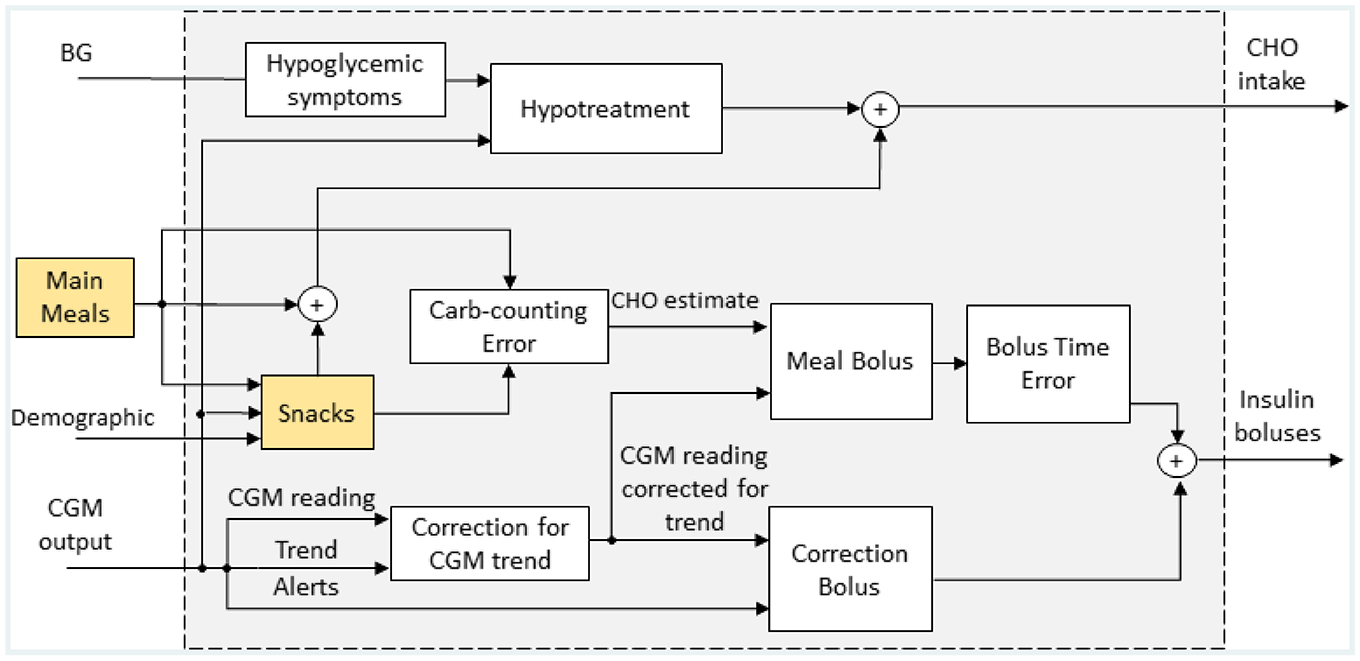
Schematic representation of the new version of the patient’s behavior and treatment decision model, included in the T1D-PDS, which embeds the new meal models developed in this work (yellow boxes). The diagram is adapted from Visentin et al.¹⁵ T1D-PDS, Type 1 Diabetes Patient Decision Simulator.

Both main meals and snacks are associated with insulin meal boluses, which are calculated both on the basis of the patient’s estimate of the CHO content of the meal ( $\hat{C H O}$ ) and on the glucose concentration, measured at meal bolus time, using the patient’s carbohydrate-to-insulin ratio and the correction factor.³⁸ The estimated $\hat{C H O}$ is simulated by implementing the nonlinear model developed in Roversi et al³⁹ which takes into account the CHO amount and the type of meal. The model of meal bolus administration time, already used in the T1D-PDS to simulate early/delayed main meal insulin administrations that commonly occur in real life, is extended to the snacks.

Once the models have been incorporated into the T1D-PDS, they are assessed through simulation. To demonstrate the reliability of their realizations, we simulated 100 virtual subjects for seven days and compared the meal-related outcomes with the real data used in this work. Assessment metrics were: number of snacks per day (# snack/day), frequency of days with at least one snack (freq_S), time between a snack and the previous main meal (Δ_mm-s), total CHO ingested per day (CHO/day), CHO ingested per day as breakfast (CHO_B/day), lunch (CHO_L/day), dinner (CHO_D/day), and snack (CHO_S/day).

Results

Table 2 shows, in median [25th-75th percentiles], the MAD computed between the EDF of TE data and the EDF of the hypothesized models, whose parameters were estimated over the TR, for 100 different TR-TE splits. For each column, the lowest MAD median value is reported in bold. Breakfast and snack CHO amount were modelled by gamma distributions, dinner CHO amount was modelled by loglogistic distributions, lunch CHO amount and breakfast time were modelled by lognormal distributions, and time between breakfast-lunch and time between lunch-dinner were modelled by GEV distributions.

Table 2.

Comparison of Candidate Models According to MAD.

PDF model	Variable
PDF model	Breakfast CHO amount	Lunch CHO amount	Dinner CHO amount	Snack CHO amount	Breakfast time	Time breakfast-lunch	Time lunch-dinner
Gaussian	0.119 [0.107-0.131]	0.134 [0.119-0.147]	0.145 [0.135-0.155]	0.164 [0.141-0.181]	0.088 [0.077-0.099]	0.048 [0.039-0.058]	0.095 [0.083-0.116]
Lognormal	0.091 [0.078-0.102]	0.072 [0.065-0.083]	0.071 [0.064-0.079]	0.123 [0.104-0.130]	0.073 [0.063-0.081]	0.074 [0.057-0.088]	0.135 [0.125-0.157]
Loglogistic	0.085 [0.077-0.094]	0.081 [0.074-0.091]	0.071 [0.063-0.081]	0.090 [0.078-0.121]	0.079 [0.072-0.087]	0.059 [0.053-0.071]	0.092 [0.083-0.104]
Gamma	0.078 [0.071-0.086]	0.080 [0.072-0.092]	0.087 [0.076-0.098]	0.087 [0.079-0.102]	0.077 [0.067-0.086]	0.061 [0.045-0.074]	0.123 [0.112-0.145]
GEV	0.082 [0.073-0.091]	0.081 [0.073-0.090]	0.072 [0.065-0.084]	0.095 [0.082-0.114]	0.074 [0.064-0.082]	0.043 [0.037-0.053]	0.063 [0.056-0.081]
t-Student	0.104 [0.095-0.118]	0.127 [0.110-0.140]	0.096 [0.087-0.104]	0.132 [0.113-0.151]	0.088 [0.077-0.099]	0.048 [0.039-0.058]	0.077 [0.068-0.099]
Exponential	0.316 [0.310-0.325]	0.289 [0.282-0.296]	0.302 [0.297-0.309]	0.207 [0.193-0.217]	0.498 [0.492-0.498]	0.403 [0.356-0.410]	0.421 [0.416-0.427]
Inverse Gaussian	0.097 [0.082-0.109]	0.073 [0.065-0.086]	0.079 [0.071-0.087]	0.208 [0.190-0.219]	0.074 [0.063-0.080]	0.078 [0.062-0.092]	0.141 [0.131-0.162]
Logistic	0.096 [0.087-0.105]	0.102 [0.093-0.115]	0.108 [0.086-0.118]	0.127 [0.111-0.146]	0.084 [0.073-0.092]	0.057 [0.049-0.068]	0.072 [0.063-0.087]
Uniform	0.324 [0.317-0.334]	0.350 [0.342-0.361]	0.456 [0.450-0.465]	0.450 [0.433-0.466]	0.312 [0.309-0.323]	0.190 [0.182-0.193]	0.269 [0.259-0.230]

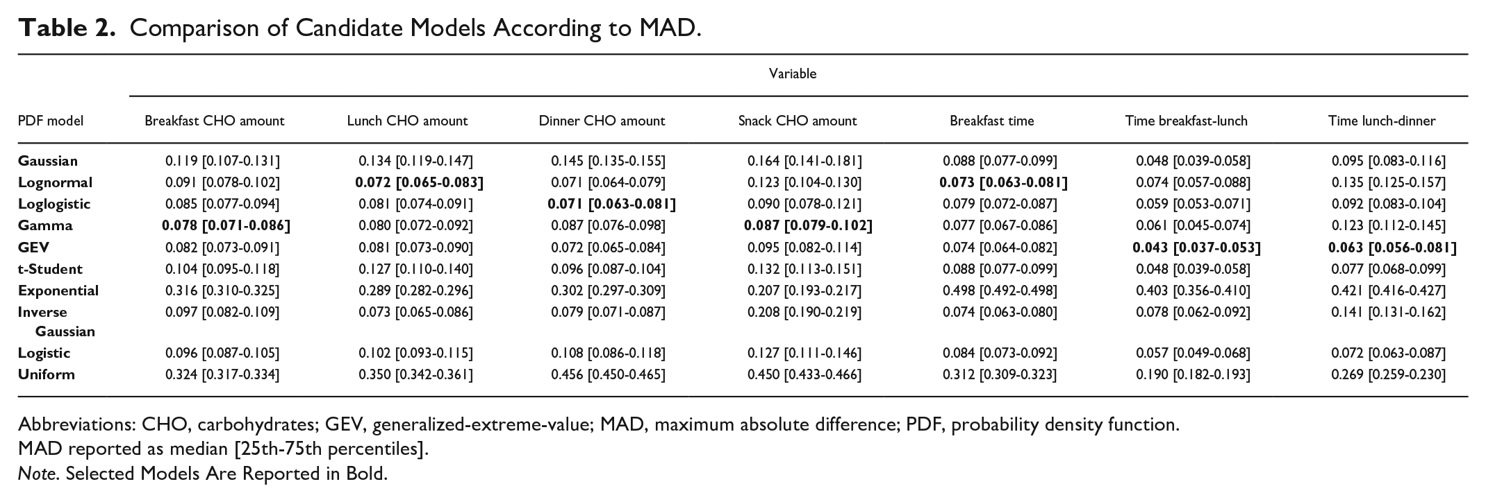
Abbreviations: CHO, carbohydrates; GEV, generalized-extreme-value; MAD, maximum absolute difference; PDF, probability density function.

MAD reported as median [25th-75th percentiles].

Note. Selected Models Are Reported in Bold.

The final models’ parameters estimated on the whole dataset are reported in the third column of Table 3. The final PDF models were plotted versus the histogram of the entire dataset in Figure 2: they replicate the shapes of the histograms well. This claim was further assessed by observing the quantile-quantile plot of the entire dataset vs the selected PDF models, reported, for each variable, in Figure 3. Indeed, since the plots approximately lay on a line, the selected PDF models were confirmed as being suitable to describe the data. Furthermore, the EDFs of 100 random samples generated by the final models and the EDF of the entire respective dataset are reported in Figure 4. The EDF of the data represents the mean of the 100 simulated EDFs quite well, for all the variables analyzed, so the models obtained had been able to mimic the shape of the distributions of the data, adding credible variability.

Table 3.

Parameters of the PDF Models of Meal CHO Content and Main Meal Time Variability.

Variable	Selected PDF model	Estimated parameters
Breakfast CHO amount	Gamma	$α = 5.290; λ = 7.696$
Lunch CHO amount	Lognormal	$μ = 3.884; σ = 0.518$
Dinner CHO amount	Loglogistic	$α = 0.284; β = 3.977$
Snack CHO amount	Gamma	$α = 2.060; λ = 11.88$
Breakfast time	Lognormal	$μ = 2.078; σ = 0.175$
Time between breakfast-lunch	GEV	$μ = 282.9; σ = 79.98; ξ = - 0.320$
Time between lunch-dinner	GEV	$μ = 374.9; σ = 84.86; ξ = - 0.472$

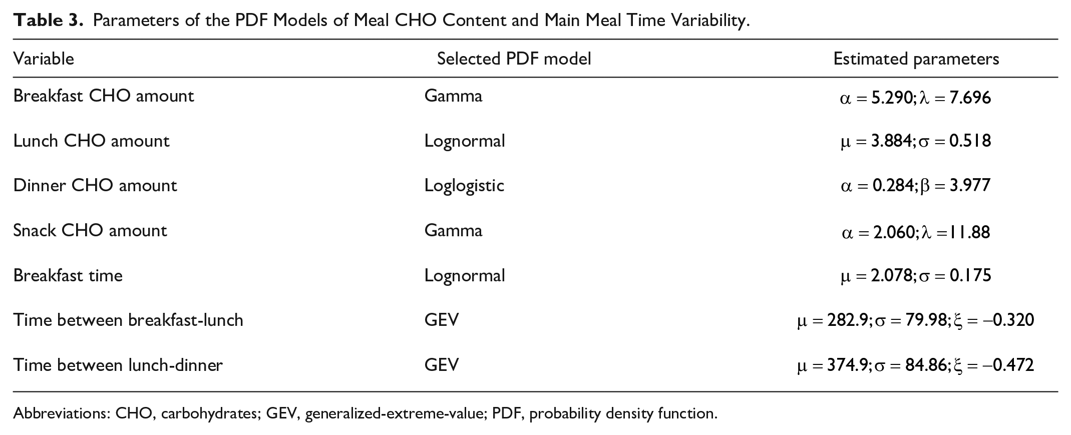
Abbreviations: CHO, carbohydrates; GEV, generalized-extreme-value; PDF, probability density function.

Figure 2.

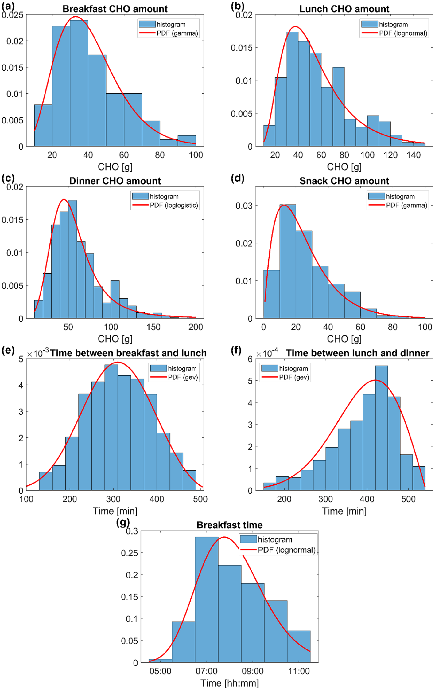
Histograms (blue) and final PDF models (red) of the following data: breakfast CHO amount (a), lunch CHO amount (b), dinner CHO amount (c), snack CHO amount (d), time between breakfast and lunch (e), time between lunch and dinner (f), breakfast time (g). CHO, carbohydrates; PDF, probability density function.

Figure 3.

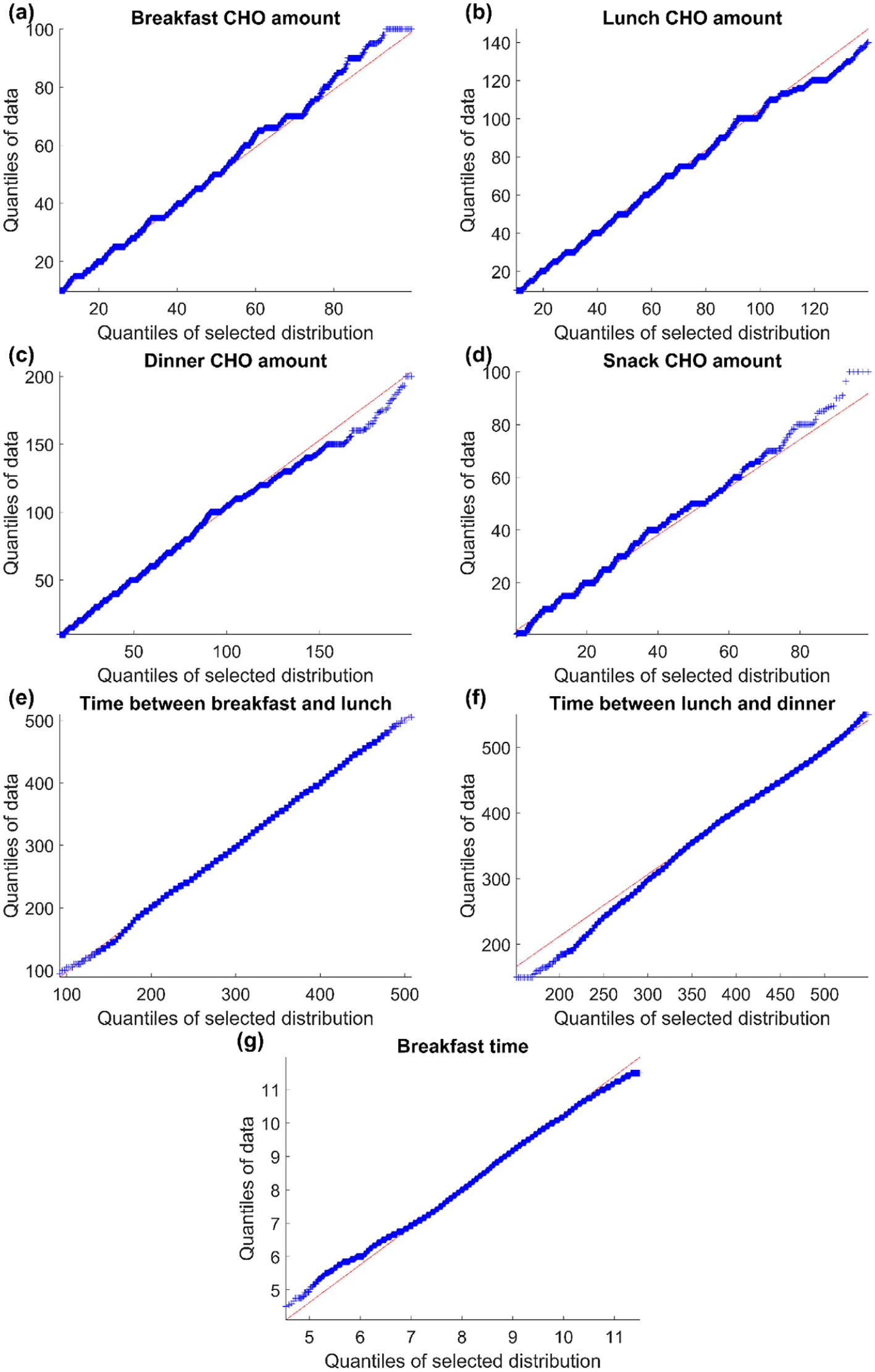
Quantile-quantile plot of data (y axis) and final PDF model (x axis) of the following variables: breakfast CHO amount (a), lunch CHO amount (b), dinner CHO amount (c), snack CHO amount (d), time between breakfast and lunch (e), time between lunch and dinner (f), breakfast time (g). The red line represents the expected quantiles of the specified PDF model. CHO, carbohydrates; PDF, probability density function.

Figure 4.

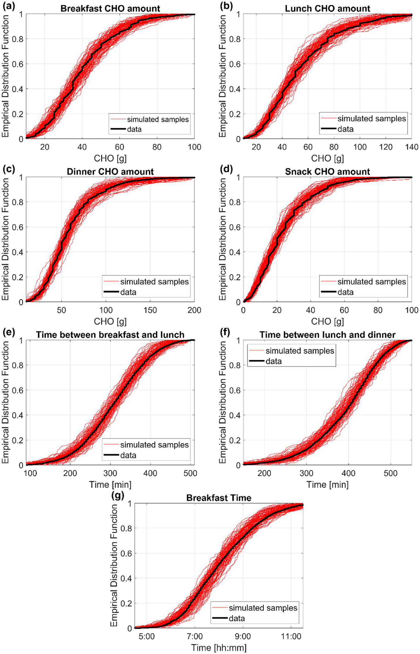
EDFs of data (black) and of 100 randomly simulated samples (red) from the final models selected for the following variables: breakfast CHO amount (a), lunch CHO amount (b), dinner CHO amount (c), snack CHO amount (d), time between breakfast and lunch (e), time between lunch and dinner (f), breakfast time (g). CHO, carbohydrates; EDFs, empirical distribution functions.

Regarding the SVM model for predicting future snacks, the feature selection step resulted in a ranked feature list of predictors and an average classification performance curve. The former was reported in Table 4, with the Borda score (second column) for each feature (first column). The latter is shown in panel (a) of Figure 5. The maximum value of the AUROC average is 0.774, which was obtained using the optimum number of features, n_opt = 7 (blue dot in Figure 5(a)). Therefore, the top seven features of the aggregated ranked list (rows in bold in Table 4), selected as the subgroup of features providing the best AUROC results, are: time of the observation window, time from the last meal intake before the observation window, subject’s age, subject’s BW, CHO amount of the last meal intake before the observation window, sum of the CHO consumed in the previous six hours before the observation window, and mean CGM in the previous one hour before the observation window.

Table 4.

Ranking of Candidate Predictors According to the Borda Score. Selected Predictors Reported in Bold.

Candidate predictors	Borda score
Time of the observation window	214
Time from the last meal intake	209
Patient’s age	196
Patient’s BW	194
CHO amount of the last meal intake	126
CHO consumed in the previous six hours	119
Mean CGM in the previous one hour	116
CHO consumed in the previous four hours	99
First CGM of the observation window	79
Mean CGM in the previous six hours	71
CHO consumed in the previous one hour	57
Rate-of-change in the previous one hour	49
Mean CGM in the previous four hours	31

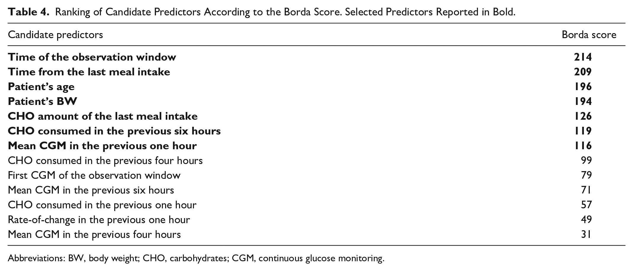
Abbreviations: BW, body weight; CHO, carbohydrates; CGM, continuous glucose monitoring.

Figure 5.

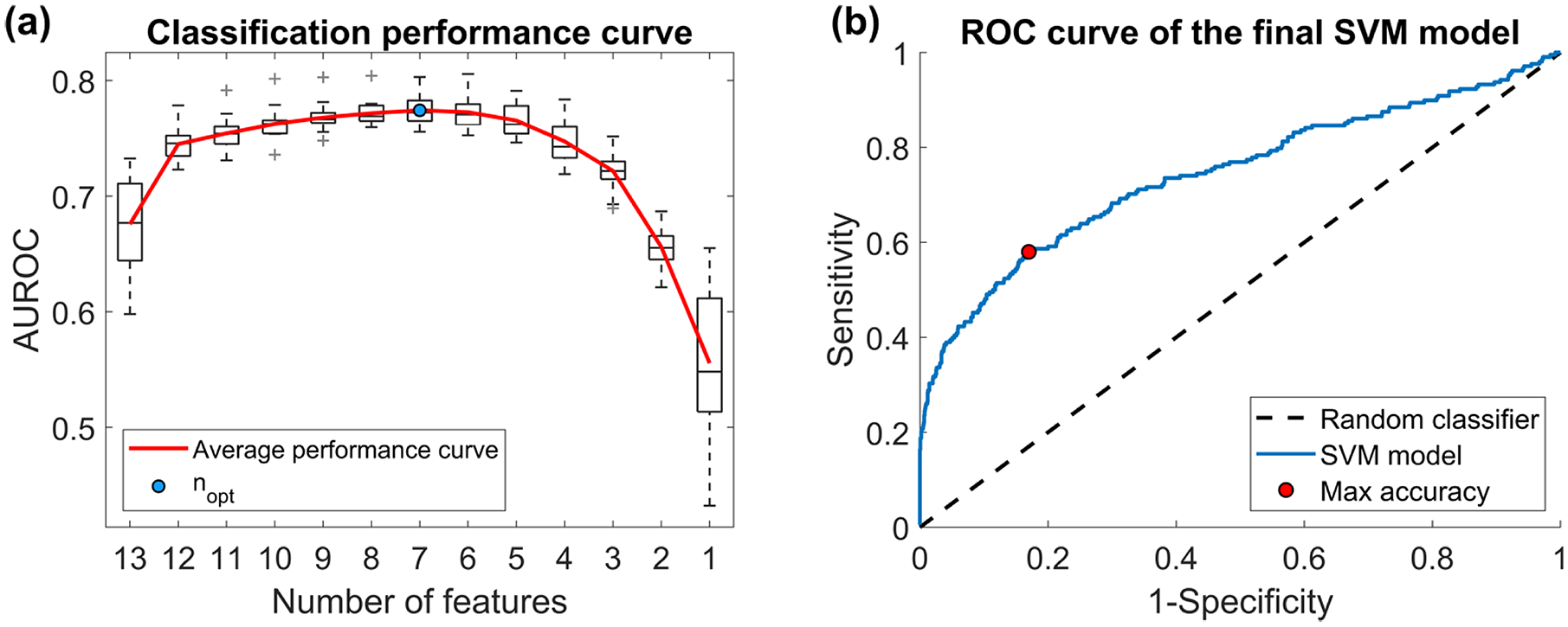
Performance curves for snack classification. Panel (a) AUROC values resulting from SVM models with different numbers of features. The average classification performance curve (red) is obtained by averaging the AUROC values over the 20-fold CV. The maximum value of the curve reflects the optimal number of features (blue dot). Panel (b) ROC curve of final SVM model (blue) and of the random classifier (dashed black line). The red dot indicates the sensitivity and specificity values at the maximum accuracy. AUROC, receiving operating characteristic curve; SVM, support vector machine.

Lastly, the SVM model containing the selected features was trained on the whole TR and evaluated on the TE, thus obtaining the ROC curve depicted in panel (b) of Figure 5. The resulting AUROC is equal to 0.754. Accuracy, sensitivity, and specificity were also computed as further performance metrics.⁴⁰ In order to maximize the accuracy, a threshold of 0.100 on the posterior probability was chosen. This threshold provides an accuracy of 0.800. The corresponding values of sensitivity and specificity are 0.592 and 0.830, respectively, and are marked by a red dot in Figure 5(b).

After embedding the models developed into the T1D-PDS, a total of 2560 meals were generated: 2100 main meals and 460 snacks. In order to assess whether the models could capture real-world data variability, in Figure 6, the distributions of CHO_B/day (panel a), CHO_L/day (panel b), CHO_D/day (panel c), CHO_S/day (panel d), #snack/day (panel e), Δ_mm-s (panel f), CHO/day (panel g) are shown through boxplot representation for both real data (label “Data”) and simulated data (label “Sim”). The metrics present similar distributions in real and simulated datasets. In Table 5, we report both the median and the interquartile range of these metrics, calculated on real data (second column) and simulated data (third column) and the P value of the two-tailed Mann-Whitney U-test, comparing metric medians in real data versus simulated data (fourth column). According to the test with 5% significance level, no statistically significant difference was found between the median outcomes of real data vs simulated data. Finally, freq_S was computed, both on real and simulated data, as the percentage of days in which at least one snack was consumed. It was equal to 71.23% for real data and 66.42% for simulated data.

Figure 6.

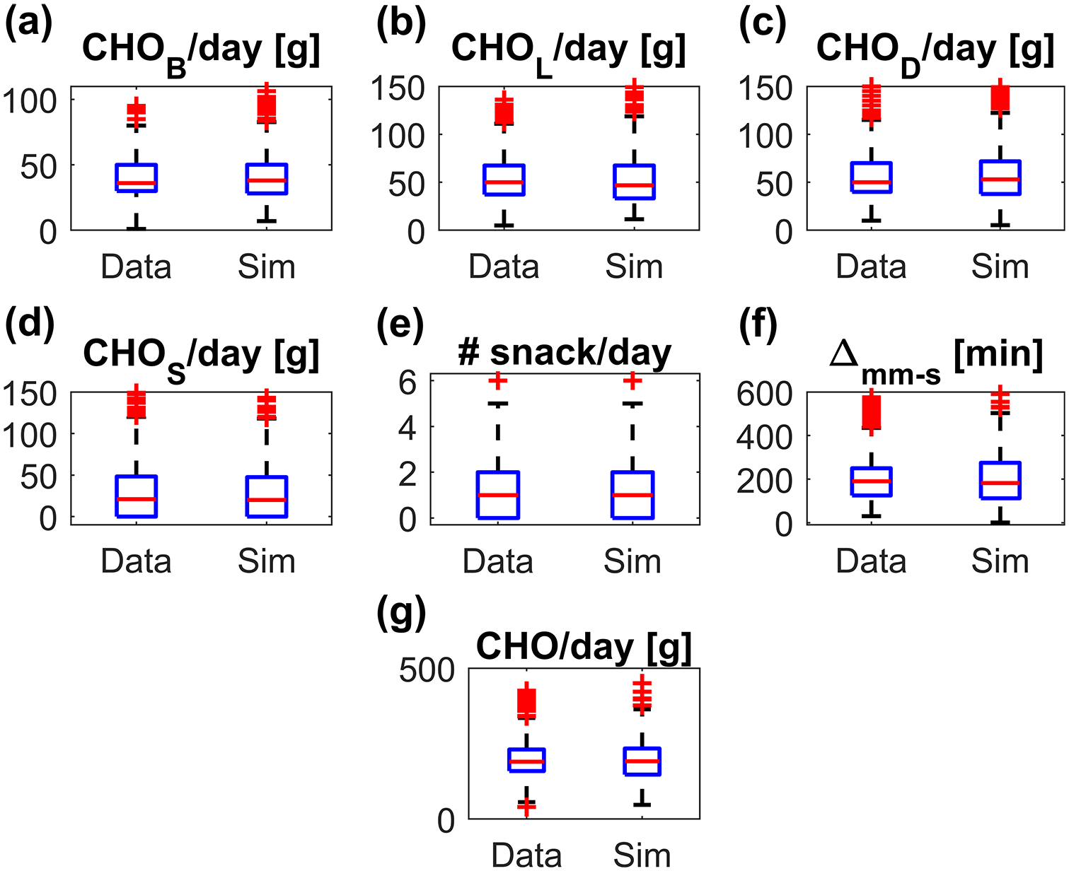
Boxplot representation of the distributions of CHO_B/day (a), CHO_L/day (b), CHO_D/day (c), CHO_S/day (d), #snack/day (e), Δ_mm-s (f), CHO/day (g), obtained on real data (label “Data”) and simulated data (label “Sim”). The red horizontal line represents median, the blue box marks the interquartile range, dashed black lines are the whiskers and the red stars indicate outliers. CHO, carbohydrates.

Table 5.

Meal Outcomes of Real Data Versus Simulated Data.

Metric	Real data	Simulated data	P value
CHO_B/day [g]	36 [30-50]	38 [28-50]	.3752
CHO_L/day [g]	50 [37-68]	46 [33-68]	.3530
CHO_D/day [g]	50 [40-70]	53 [38-72]	.4416
CHO_S/day [g]	0 [21-48]	0 [20.0-48]	.3098
#snack/day	0 [1-2]	0 [1-2]	.4708
Δ_mm-s [min]	190 [125-250]	182 [112-275]	.4618
CHO/day [g]	190 [159-231]	191 [147-234]	.2488

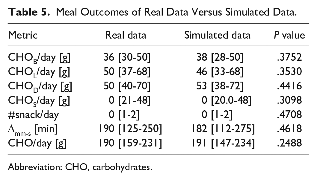
Abbreviation: CHO, carbohydrates.

Conclusion

Existing T1D simulators are not equipped with realistic descriptions of some behavioral aspects that can remarkably affect glycemic control. In this work, by leveraging a dataset involving 32 T1D individuals monitored up to six months, we developed models to describe meal amount and timing variability under free-living conditions. We obtained eight separate PDF models to describe the CHO amount of main meals (ie, breakfast, lunch, and dinner) and snacks and the time between consecutive main meals. We also derived an SVM model to predict the probability that a snack will be consumed in a future time window, based on predictors collected back in time and linked to time and CHO amount of previous meal intakes, CGM, time of the day, and the subject’s demographic data. The models developed were incorporated into the recent T1D-PDS as two sub-modules. The first one, describing the main meals, is a population model; thus it is based on the assumption that the distribution of CHO amount ingested as main meals is the same for every virtual patient. The second one, triggering the snacks during the day, considers subject-specific covariates; thus it allows to create differences in the total daily ingested CHO amount between virtual subjects. The reliability of the newly developed model was assessed by comparing the simulated meals of 100 virtual subjects to the meals collected in the study used in this work. The comparison highlighted good agreement between the metrics calculated on real and on simulated data.

Of course, the characteristics of the dataset available to us made it clear that there is room for improvement. For instance, using the same methodology that we proposed on a much larger dataset would make it possible to link meal habits to the cultural eating habits of the country of reference of the subject. Then, the models could be refined by capturing the temporal patterns of patients’ meal behavior at various time scales (eg, working days vs weekend, different seasons, etc.). Future developments could also include developing personalized models for main meal CHO amount and timing, modelling meal duration, and determining the probability of missed main meals. Finally, when absorption models of complex CHO intakes will be developed and embedded in the T1D-PDS, behavioral model to realistically simulate the meal composition could also be investigated. In conclusion, the T1D-PDS, enhanced with the models developed in this work, is expected to allow investigators to perform more reliable and insightful ISCTs. For instance, part of our work currently underway in the Hypo-RESOLVE project⁴¹ concerns the use of the T1D-PDS to quantify the impact of different behavioral factors in inducing hypoglycemia.

Supplemental Material

Supplemental_material_PDF – Supplemental material for Mathematical Models of Meal Amount and Timing Variability With Implementation in the Type-1 Diabetes Patient Decision Simulator

Supplemental material, Supplemental_material_PDF for Mathematical Models of Meal Amount and Timing Variability With Implementation in the Type-1 Diabetes Patient Decision Simulator by Nunzio Camerlingo, Martina Vettoretti, Simone Del Favero, Andrea Facchinetti and Giovanni Sparacino in Journal of Diabetes Science and Technology

Footnotes

Appendix

The strategy used to classify meal data as main meal or snack was based on the CHO amount and the time registered by subjects during the trial: when two or more meals (eg, lunch and snack) fell into the same time window, the meal with the biggest CHO amount among them was classified as main meal, while the others were considered snacks. Even if sometimes this classification rule might mistake a small meal for a snack, having an exact meal labeling was not crucial for the final purpose of allowing the T1D-PDS to simulate CHO intakes during the hours of the day in a plausible way, which reflects what is observed in real data.

Anyway, a sensitivity analysis was performed to quantify the impact of the possible labeling errors. Specifically, as confusing one main meal with another main meal (e.g., a lunch with a dinner) is very unlikely, the analysis was focused on assessing the impact of the initial choice of selecting the main meal in each time window as the one with the biggest CHO amount among the meals in that time window. The procedure of the sensitivity analysis is described as follows.

For each time window including more than one meal, if the absolute difference between two largest meals was lower than or equal to a fixed threshold (ΔCHO ≤ 10%, 20%, 30%), the two meal labels were willingly exchanged, ie, the second largest meal became the “main meal” and the largest meal was labeled as a “snack.” This was performed for the 10%, 50%, and 100% of the snacks, randomly selected. Then, the PDF models selected in the work for the snack CHO amount (gamma), breakfast CHO amount (gamma), lunch CHO amount (lognormal), dinner CHO amount (loglogistic), time between breakfast and lunch (GEV), and time between lunch and dinner (GEV) were re-trained on the dataset with the new labels, and the newly obtained distributions were compared against those obtained with the original labeling, both by visual inspection (Supplemental Figures 1–3) and by comparison of their mean and standard deviation. Supplemental Figure 1 reports the PDF models obtained with the original labeling (black), the ones obtained with misclassification of 10% (dashed blue), 50% (dashed green), 100% (dashed red) of the snacks, for CHO amount of snack (panel A), breakfast (panel B), lunch (panel C), dinner (panel D), and the time between breakfast-lunch (panel E) and lunch-dinner (panel F), using ΔCHO ≤ 10%. Similar figures are obtained for the scenarios ΔCHO ≤ 20% (Supplemental Figure 2) and ΔCHO ≤ 30% (Supplemental Figure 3).

As expected, a limited number of errors in the labeling step does not significantly impact on the PDF models shape. Slight differences can be appreciated in the ΔCHO ≤ 30% scenario: the mean of the snack CHO amount increases and the mean of lunch CHO amount decrease, thus not affecting, on average, the CHO amount consumed in the time window. The distributions of time between breakfast-lunch and lunch-dinner are, expectedly, the least affected by the mislabeling.

Quantitative considerations can be drawn from Supplemental Table 1, reporting mean and standard deviation of the distributions obtained after the mislabeling and, in the last column, mean and standard deviation of the original distributions. In the ΔCHO ≤ 30% scenario, with 100% mislabeled snacks, the mean of the snack CHO amount only differs of about 5 g from the original mean, as well as the mean of the dinner CHO amount. The mean values of time between breakfast-lunch and lunch-dinner differ of less than five minutes from the original distributions. Therefore, we can conclude that labeling errors do not affect the distributions shape and, consequently, the results of the ISCT are insensitive to this kind of error.

Declaration of Conflicting Interests

The author(s) declared no potential conflicts of interest with respect to the research, authorship, and/or publication of this article.

Funding

The author(s) disclosed receipt of the following financial support for the research, authorship, and/or publication of this article: This study is part of the Hypo-RESOLVE project. The project has received funding from the Innovative Medicines Initiative 2 Joint Undertaking (JU) under grant agreement No. 777460. The JU receives support from the European Union’s Horizon 2020 research and innovation program and EFPIA and T1D Exchange, JDRF, International Diabetes Federation (IDF), The Leona M. and Harry B. Helmsley Charitable Trust.

ORCID iDs

Nunzio Camerlingo

Simone Del Favero

Giovanni Sparacino

Supplemental Material

Supplemental material for this article is available online.

References

Wilinska

Hovorka

Simulation models for in silico testing of closed-loop glucose controllers in type 1 diabetes. Drug Discov Today Dis Model. 2008;5(4):289-298.

Camerlingo

Vettoretti

Del Favero

Cappon

Sparacino

Facchinetti

A real-time continuous glucose monitoring-based algorithm to trigger hypotreatments to prevent/mitigate hypoglycemic events. Diabetes Technol Ther. 2019;21(11):644-655.

Breton

Hinzmann

Campos-Nañez

Riddle

Schoemaker

Schmelzeisen-Redeker

Analysis of the accuracy and performance of a continuous glucose monitoring sensor prototype: an in-silico study using the UVA/PADOVA type 1 diabetes simulator. J Diabetes Sci Technol. 2017;11(3):545-552.

Schiavon

Dalla Man

Cobelli

Insulin sensitivity index-based optimization of insulin to carbohydrate ratio: in silico study shows efficacious protection against hypoglycemic events caused by suboptimal therapy. Diabetes Technol Ther. 2018;20(2):98-105.

Rehman

Munawar

Akash

MSH

, et al. Hesperidin improves insulin resistance via down-regulation of inflammatory responses: biochemical analysis and in silico validation. PLoS One. 2020;15(1):e0227637.

Schiavon

Visentin

Giegerich

, et al. In silico head-to-head comparison of insulin glargine 300 U/mL and insulin degludec 100 U/mL in type 1 diabetes. Diabetes Technol Ther. 2020;22(8):553-561.

Dasgupta

Bandyopadhyay

Ray

, et al. Catestatin improves insulin sensitivity by attenuating endoplasmic reticulum stress: in vivo and in silico validation. Comput Struct Biotechnol J. 2020;18:464-481.

Kovatchev

Breton

Dalla Man

Cobelli

In silico preclinical trials: a proof of concept in closed-loop control of type 1 diabetes. J Diabetes Sci Technol. 2009;3:44-55.

Bajard

Chabaud

Cornu

, et al. An in silico approach helped to identify the best experimental design, population, and outcome for future randomized clinical trials. J Clin Epidemiol. 2016;69:125-136.

10.

Herrero

Bondia

Adewuyi

, et al. Enhancing automatic closed-loop glucose control in type 1 diabetes with an adaptive meal bolus calculator: in silico evaluation under intra-day variability. Comput Methods Programs Biomed. 2017;146:125-131.

11.

Toffanin

Visentin

Messori

Di Palma

Magni

Cobelli

Toward a run-to-run adaptive artificial pancreas: in silico results. IEEE Trans Biomed Eng. 2018;65(3):479-488.

12.

Wilinska

Chassin

Acerini

Allen

Dunger

Hovorka

Simulation environment to evaluate closed-loop insulin delivery systems in type 1 diabetes. J Diabetes Sci Technol. 2010;4(1):132-144.

13.

Viceconti

Henney

Morley-Fletcher

In silico clinical trials: how computer simulation will transform the biomedical industry. Int J Clin Trials. 2016;3(2):37-46.

14.

Meneghetti

Susto

Del Favero

Detection of insulin pump malfunctioning to improve safety in artificial pancreas using unsupervised algorithms. J Diabetes Sci Technol. 2019;13(5):1065-1076.

15.

Visentin

Campos-Náñez

Schiavon

, et al. The UVA/Padova type 1 diabetes simulator goes from single meal to single day. J Diabetes Sci Technol. 2018;12(2):273-281.

16.

Hovorka

Shojaee-Moradie

Carroll

, et al. Partitioning glucose distribution/transport, disposal, and endogenous production during IVGTT. Am J Physiol Endocrinol Metab. 2002;282(5):992-1007.

17.

Rashid

Samadi

Sevil

, et al. Simulation software for assessment of nonlinear and adaptive multivariable control algorithms: glucose–insulin dynamics in type 1 diabetes. Comput Chem Eng. 2019;130:106565.

18.

Fabietti

Canonico

Federici

Benedetti

Sarti

Control oriented model of insulin and glucose dynamics in type 1 diabetics. Med Biol Eng Comput. 2006;44(1-2):69-78.

19.

Cameron

Niemeyer

Bequette

BW.

Extended multiple model prediction with application to blood glucose regulation. J Process Control. 2012;22(8):1422-1432.

20.

Vettoretti

Facchinetti

Sparacino

Cobelli

Type-1 diabetes patient decision simulator for in silico testing safety and effectiveness of insulin treatments. IEEE Trans Biomed Eng. 2018;65(6):1281-1290.

21.

Cappon

Vettoretti

Sparacino

Facchinetti

Continuous glucose monitoring sensors for diabetes management: a review of technologies and applications. Diabetes Metab J. 2019;43(4):383-397.

22.

Garcia-Tirado

Zuluaga-Bedoya

Breton

MD.

Identifiability analysis of three control-oriented models for use in artificial pancreas systems. J Diabetes Sci Technol. 2018;12(5):937-952.

23.

Kropff

Del Favero

Place

, et al. 2 month evening and night closed-loop glucose control in patients with type 1 diabetes under free-living conditions: a randomised crossover trial. Lancet Diabetes Endocrinol. 2015;3(12):939-947.

24.

Renard

Farret

Kropff

, et al. Day-and-night closed-loop glucose control in patients with type 1 diabetes under free-living conditions:results of a single-arm 1-month experience compared with a previously reported feasibility study of evening and night at home. Diabetes Care. 2016;39(7):1151-1160.

25.

Messori

Kropff

Del Favero

, et al. Individually adaptive artificial pancreas in subjects with type 1 diabetes: a one-month proof-of-concept trial in free-living conditions. Diabetes Technol Ther. 2017;19(10):560-571.

26.

Keith-Hynes

Guerlain

Mize

, et al. DiAs user interface: a patient-centric interface for mobile artificial pancreas systems. J Diabetes Sci Technol. 2013;7:141626.

27.

Kant

Graubard

BI.

40-year trends in meal and snack eating behaviors of American adults. J Acad Nutr Diet. 2015;115(1):50-63.

28.

Zhou

Erdem

Shi

Comprehensive evaluation of wind speed distribution models: a case study for North Dakota sites. Energy Convers Manag. 2010;51(7):1449-1458.

29.

Usta

Kantar

YM.

Analysis of some flexible families of distributions for estimation of wind speed distributions. Appl Energy. 2012;89(1):355-367.

30.

Shabri

Ariff

NM.

On selection of probability distributions of annual maximum daily rainfalls using TL-moments. Mat Malays J Ind Appl Math. 2010;26:137-151.

31.

Luor

DC.

A comparative assessment of data standardization on support vector machine for classification problems. Intell Data Anal. 2015;19(3):529-546.

32.

Soman

Sathiya

Suganthi

Classification of stress of automobile drivers using radial basis function kernel support vector machine. Presentation at: 2014 International Conference on Information Communication and Embedded Systems, ICICES 2014; 2014; IEEE:1-5.

33.

Cho

Lee

Chee

Kim

SI.

Nonlinear support vector machine visualization for risk factor analysis using nomograms and localized radial basis function kernels. IEEE Trans Inf Technol Biomed. 2008;12(2):247-256.

34.

Francescatto

Chierici

Dezfooli

Zandonà

Jurman

Furlanello

Multi-omics integration for neuroblastoma clinical endpoint prediction. Biol Direct. 2018;13(5):1-12.

35.

Guyon

Weston

Barnhill

Vapnik

Gene selection for cancer classification using support vector machines. Mach Learn. 2002;46(1-3):389-422.

36.

Gysels

Renevey

Celka

SVM-based recursive feature elimination to compare phase synchronization computed from broadband and narrowband EEG signals in brain-computer interfaces. Signal Process. 2005;85(11):2178-2189.

37.

Jurman

Merler

Barla

Paoli

Galea

Furlanello

Algebraic stability indicators for ranked lists in molecular profiling. Bioinformatics. 2008;24(2):258-264.

38.

Davidson

Hebblewhite

Steed

Bode

Analysis of guidelines for basal-bolus insulin dosing: basal insulin, correction factor, and carbohydrate-to-insulin ratio. Endocr Pract. 2008;14(9):1095-1101.

39.

Roversi

Vettoretti

Del Favero

Facchinetti

Sparacino

. Modeling carbohydrate counting error in type 1 diabetes management [published online ahead of print March 30, 2020]. Diabetes Technol Ther. doi:10.1089/dia.2019.0502

40.

Baldi

Brunak

Chauvin

Andersen

Nielsen

Assessing the accuracy of prediction algorithms for classification: an overview. Bioinformatics. 2000;26(5):412-424.

41.

Hypo-RESOLVE. Hypoglycaemia—REdefining SOLutions for better liVEs. https://hypo-resolve.eu/. Accessed May 9, 2020.

Supplementary Material

Please find the following supplemental material available below.

For Open Access articles published under a Creative Commons License, all supplemental material carries the same license as the article it is associated with.

For non-Open Access articles published, all supplemental material carries a non-exclusive license, and permission requests for re-use of supplemental material or any part of supplemental material shall be sent directly to the copyright owner as specified in the copyright notice associated with the article.

0.00 MB

0.33 MB