Sage Journals: Discover world-class research

Abstract

Background:

Hypoglycemia is a serious health concern in youth with type 1 diabetes (T1D). Real-time data from continuous glucose monitoring (CGM) can be used to predict hypoglycemic risk, allowing patients to take timely intervention measures.

Methods:

A machine learning model is developed for probabilistic prediction of hypoglycemia (<70 mg/dL) in 30- and 60-minute time horizons based on CGM datasets obtained from 112 patients over a range of 90 days consisting of over 1.6 million CGM values under normal living conditions. A comprehensive set of features relevant for hypoglycemia are developed and a parsimonious subset with most influence on predicting hypoglycemic risk is identified. Model performance is evaluated both with and without contextual information on insulin and carbohydrate intake.

Results:

The model predicted hypoglycemia with >91% sensitivity for 30- and 60-minute prediction horizons while maintaining specificity >90%. Inclusion of insulin and carbohydrate data yielded performance improvement for 60-minute but not for 30-minute predictions. Model performance was highest for nocturnal hypoglycemia (~95% sensitivity). Shortterm (less than one hour) and medium-term (one to four hours) features for good prediction performance are identified.

Conclusions:

Innovative feature identification facilitated high performance for hypoglycemia risk prediction in pediatric youth with T1D. Timely alerts of impending hypoglycemia may enable proactive measures to avoid severe hypoglycemia and achieve optimal glycemic control. The model will be deployed on a patient-facing smartphone application in an upcoming pilot study.

Keywords

continuous glucose monitoring feature extraction machine learning hypoglycemia prediction insulin pump data carbohydrate intake

Introduction

A prevalent and feared consequence of diabetes management is severe hypoglycemia, which can result in seizures, loss of consciousness, and death. Fear of hypoglycemia is prevalent in adults with diabetes¹ and in parents of children with diabetes.² This fear is greatest during high risk activities such as sleeping, exercising, and driving,³ and often leads to more conservative glucose control, increasing the risks of hyperglycemia, which may lead to long-term micro- and macrovascular complications.^4
-6

Continuous glucose monitoring (CGM) allows frequent, automated sensor glucose readings from inter-stitial fluid in the subcutaneous tissue space. CGM has been shown to improve glycemic control and reduce glycemic excursion—decreasing both hypoglycemia and hyperglycemia.⁷ CGM can be used in combination with insulin pumps via sensor augmented pump therapy.⁸ Real-time CGM devices provide real-time auditory alerts for glucose excursions above or below customized thresholds but do not yet predict impending hypoglycemic events (<70 mg/dL).

Bremer and Gough⁹ first attempted to predict future glucose levels using past glucose values in 1999. Since then, many researchers have developed models for predicting hypoglycemia using statistical and machine learning methods. These studies can be broadly divided into classification-based approaches for predicting future hypoglycemic events and regression-based approaches for predicting future glucose values. Although some studies^10,11 provide comparative analysis of various methodologies, detailed comparison is nontrivial due to differences in CGM sensors and sampling intervals, preprocessing steps for CGM data, variations in hypoglycemic event definition, and data collection (synthetically generated, controlled study, free-living conditions).¹² Because our work emphasizes feature extraction, the following review will focus on features used for prediction.

Studies have tried to include features from demographic data such as age, gender, body mass index, hemoglobin A1c (HbA1c), duration of diabetes as well as features extracted from CGM observations in the past 30 minutes to enhance predictive capabilities.^12
-20 A 30-minute time window is often selected because autocorrelation was shown to dissipate beyond 30 minutes.²¹ Some studies also use CGM values in the previous 30 minutes as input to time-series methods such as ARIMA-ARIMAX.^16,22
-27 Owing to the ability of state-space models to better handle complex processes and have an interpretable structure, many works used methods based on state-space models to predict hypoglycemic events based on the CGM signal.^11,28
-36 Recently, some researchers have relied on the use of sequence-based neural networks to automatically infer patterns from CGM data. However, it was shown that the neural networks resulted in only marginal improvements.¹²

Cichosz et al¹³ used variability-based features extracted from CGM readings in a 30-minute window along with heart rate data. As noted by the authors, the study was limited by small sample size (n = 10 and 903 sample points). Jensen et al¹⁴ developed a model to predict nocturnal hypoglycemia using rates of glycemic change in the first, second, and third nights before the hypoglycemic event. The authors also included glycemic variability at specific intervals during the night as well as static contextual information.

Many studies have explored using meal information, insulin, and physical activity for the prediction of hypoglycemic events. Simple to highly sophisticated models have been developed to model insulin and carbohydrate absorption.^37
-40 The results, in the context of hypoglycemia prediction, have been mixed with most reporting only marginal improvement.^10,12,41
-43

Methods

Materials

The CGM datasets were obtained from 112 patients using Dexcom G6 CGM devices over a range of 90 days consisting of over 1 639 921 CGM values under normal living conditions. Corresponding insulin pump data for participants provided details on the amount of insulin administered, it’s time of delivery, and the associated carbohydrate count. Pump data was available only for 19 of the patients. Table 1 provides a profile of patients in the study.

Table 1.

Data Characteristics.

Patient baseline characteristics
	Mean ± SD	Range
Gender	Male—64; Female—48
Age (years)	12.67 ± 4.84	1–21
HbA1c (%)	7.70 ± 1.63	5–12.5
Duration of diabetes (years)	4.93 ± 4.09	0.25–19.18
Descriptive statistics: CGM metrics
	Mean ± SD	Range
Hypoglycemic values/day^a	6.2 ± 5.98	0.1–23.73
% hypoglycemic values^b	2.23 ± 2.1	0.5–12.2

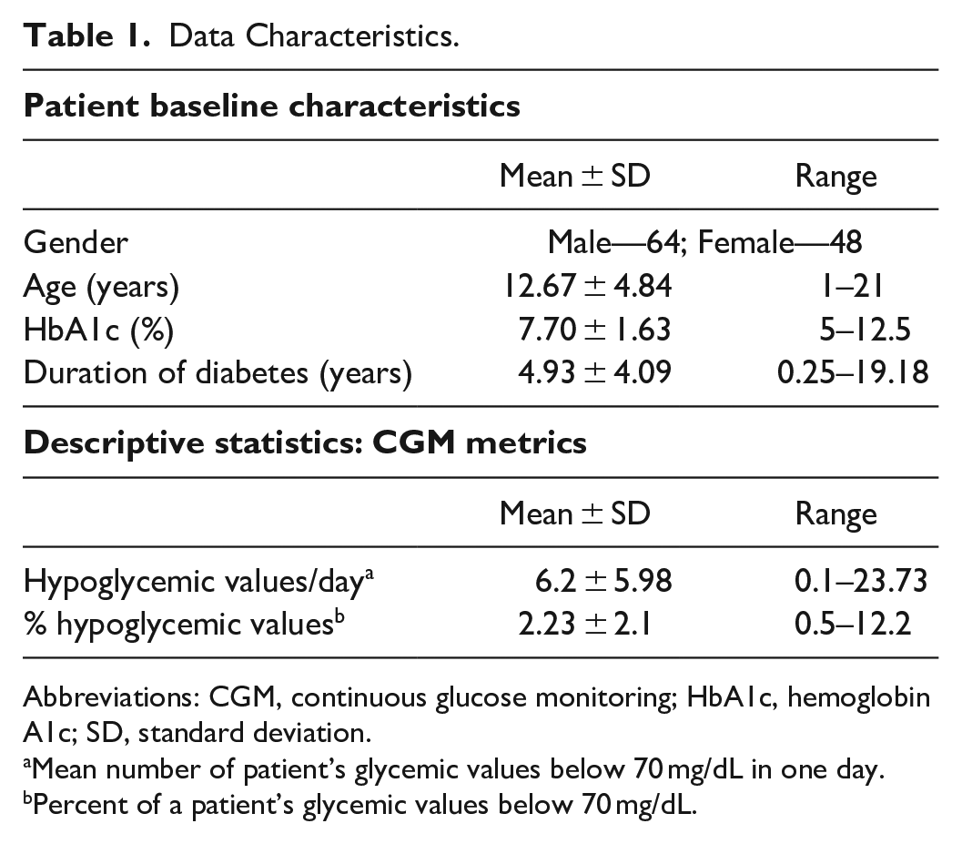
Abbreviations: CGM, continuous glucose monitoring; HbA1c, hemoglobin A1c; SD, standard deviation.

Mean number of patient’s glycemic values below 70 mg/dL in one day.

Percent of a patient’s glycemic values below 70 mg/dL.

Feature Extraction

A total of 26 features were extracted from the CGM signal based on exploratory data analysis and discussions with clinicians. Table 2 provides a description of each feature. These features are classified into seven categories:

(1) Short-term features: Short-term features capture glucose patterns within one hour before the current CGM observation.

(2) Medium-term features: Mid-term features capture glucose patterns from four hours to one hour before the current CGM observation and include features such as standard deviation and slope. Slope between two temporally ordered glucose values <X₁, X₂> is defined as (X₂ − X₁)/X₁.

(3) Long-term features: Long-term features capture glucose patterns at times exceeding four hours before the current CGM observation. These features encapsulate the long-term ability of a patient to manage glucose levels. Innovative features extracted include number of rebound lows, rebound highs, near rebound highs, and near rebound lows. We define rebound lows as events when glucose is above 200 mg/dL and then falls to below 70 mg/dL within an hour and similarly a rebound high as an event when glucose levels rise from below 70 mg/dL to above 200 mg/dL within an hour. Near rebound lows and near rebound highs are similar patterns with 90 and 180 mg/dL thresholds.

(4) Demographic features: Demographic features such as age group, gender, duration of diabetes, and the last HbA1c value were included in the analysis.

(5) Snowball effect features: To capture the accruing effects of changes over time, positive and negative glucose changes accumulated over the last two hours are considered as features.

(6) Interaction and nonlinear features: For hypoglycemia, glucose falls at higher glucose levels are not as important as glucose falls at lower glucose levels. That is, a change of 10 mg/dL is more serious when glucose is at 70 mg/dL than when glucose is at 200 mg/dL. Thus, two variables were considered with interaction between: (i) current glucose value and overall standard deviation and (ii) current glucose value and difference in the last 10 minutes. Also, square of glucose was included as a feature to introduce nonlinearity in the model.

(7) Contextual variables: Hour of day and day of week were included in the analysis to capture “seasonal” types of patterns. Figure 1 provides boxplots of CGM variations by hour for a sample patient. Insulin on board and carbohydrates were also calculated and included in the analysis. (Day of week also appeared to have importance, but a figure is not included for brevity.) Insulin on board was calculated using a linear model, which assumed insulin effects wear off in four hours (Fig. 2).⁴⁴ Carbohydrates were modeled as being absorbed at a rate of 0.5 g/min after an initial lag of 15 minutes.⁴⁵

Table 2.

Features Extracted for Prediction.

Variable	Description
Short-term features
Glucose	Actual CGM observation made at a point
diff_10	Difference between current CGM observation and the one observed 10 minutes earlier
diff_20	Difference between current CGM observation and the one observed 20 minutes earlier
diff_30	Difference between current CGM observation and the one observed 30 minutes earlier
slope_1hr	Rate of change in CGM values in past one hour
Medium-term features
sd_2hr	Standard deviation of CGM observations observed in the past two hours
sd_4hr	Standard deviation of CGM observations observed in the past four hours
slope_2hr	Rate of change in CGM in the past two hours
Long-term features
rebound_high	Number of rebound highs observed for the patient
rebound_low	Number of rebound lows observed for the patient
near_rebound_high	Number of near rebound highs observed for the patient
near_rebound_low	Number of near rebound lows observed for the patient
SD	Standard deviation of all CGM observations across the patient
time_below70	% of CGM observations below 70
time_above200	% of CGM observations above 200
Snowball effect features
pos	Sum of all increments in adjacent CGM observations in last two hours
neg	Sum of all decrements in adjacent CGM observations in past two hours
max_pos	Maximum increase in adjacent CGM observations in past two hours
max_neg	Maximum decrease in adjacent CGM observations in past two hours
Demographic features
gender	Male or female
category	Age group: (0-5), (6-10), (11-15), (16-20)
duration	Years since diabetes diagnosis
HbA1C	Last known HbA1c value
Interaction and nonlinear features
interaction 1	Interaction between glucose and SD
interaction 2	Interaction between glucose and diff_10
glucose_sq	Square of glucose value
Contextual features
Hour	Hour of the day when observation was made
day	Day of the week when observation was made
Insulin on board	Insulin remaining in the body at a time point
Carb on board	Carb remaining in the body at a time point

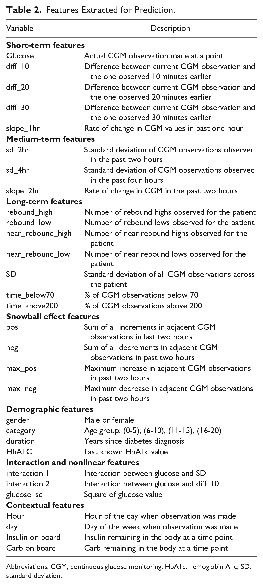
Abbreviations: CGM, continuous glucose monitoring; HbA1c, hemoglobin A1c; SD, standard deviation.

Figure 1.

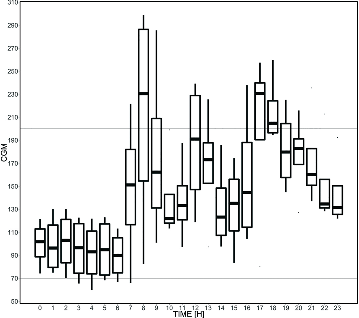
Boxplot of CGM variations by hour for a sample patient.

Figure 2.

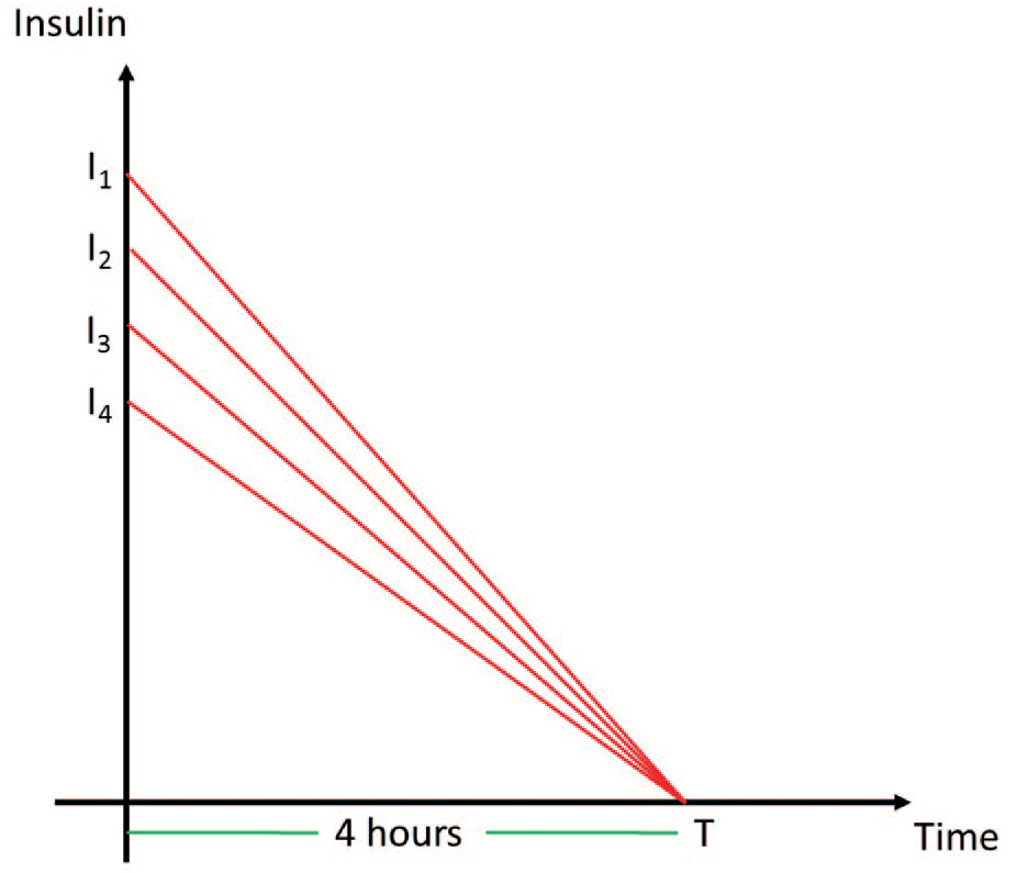
Insulin on board over time for different insulin boluses.

Machine Learning Algorithms/Methodologies

A threshold of 70 mg/dL was used to identify a hypoglycemic event (positive hypoglycemic class—class 1).^46,47 Two approaches were considered for prediction: (i) Logistic Regression (LR) and (ii) Random Forests (RF).³⁸ These two methods were selected based on their predictive capabilities in similar settings^48,49 and their ability to rate feature importance. Classifiers based on Decision Trees, Gradient Boosting, and Support Vector Machines⁵⁰ were developed, but the results obtained were at best similar to the methods short-listed.

Hypoglycemic Prediction Window

Existing studies focus prediction of hypo- and hyperglycemic events at a specific time point in the future. For example, they predict the risk of hypoglycemic events at 30 or 60 minutes from the reference time. CGM values are highly dynamic and will go through significant pattern changes in a 30-minute window. Some of these might be due to interventions such as consuming fast-acting carbohydrates and others due to normal pattern changes. Focusing on events at exactly 30 minutes in the future (34 225 hypoglycemic events) will result in ignoring clinically significant events happening “within” that 30-minute window (45 506 hypoglycemic events). It makes sense that a patient’s hypoglycemia risk within the next X minutes would have more clinical significance as a patient’s hypoglycemia risk at exactly X minutes in the future.

To accommodate this important observation and to facilitate more clinically and patient relevant predictions, we predicted the hypoglycemic risk within an interval of time into the future (0-15, 15-30, 30-45, and 45-60 minutes) (Table 3). Results for predicting at exactly 15, 30, 45, and 60 minutes were also evaluated and are presented in Table 4 for comparison.

Table 3.

Model Performance Metrics.

“Within” prediction window
Model	0-15 min		15-30 min		30-45 min		45-60 min
Model	Sensitivity	Specificity	Sensitivity	Specificity	Sensitivity	Specificity	Sensitivity	Specificity
LASSO Optimized LR	94.27	97.32	84.19	94.06	68.08	92.90	53.87	92.88
VIP Optimized RF	95.82	97.21	93.61	93.50	92.28	90.73	91.01	89.82
RF—Day	95.26	97.00	92.23	92.84	90.28	89.59	89.37	89.16
RF—Night	96.99	98.04	96.59	95.79	96.27	94.18	95.82	92.99
With Insulin and Carbohydrates on board	98.35	97.75	97.04	95.23	96.92	94.89	96.21	95.73

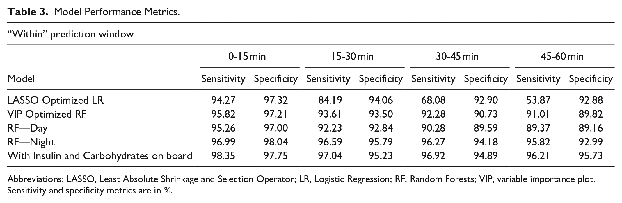
Abbreviations: LASSO, Least Absolute Shrinkage and Selection Operator; LR, Logistic Regression; RF, Random Forests; VIP, variable importance plot.

Sensitivity and specificity metrics are in %.

Table 4.

Model Performance Metrics.

“At” prediction window
Model	15 min		30 min		45 min		60 min
Model	Sensitivity	Specificity	Sensitivity	Specificity	Sensitivity	Specificity	Sensitivity	Specificity
LASSO Optimized LR	91.85	96.25	73.75	94.87	55.06	95.50	43.28	95.25
VIP Optimized RF	94.20	96.67	90.93	93.65	88.04	92.68	86.28	93.07
RF—Day	93.08	96.25	88.43	92.90	84.10	91.96	82.92	92.97
RF—Night	96.18	97.57	94.92	95.85	94.77	94.44	93.85	93.97

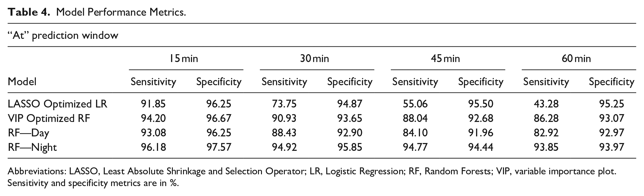
Abbreviations: LASSO, Least Absolute Shrinkage and Selection Operator; LR, Logistic Regression; RF, Random Forests; VIP, variable importance plot.

Sensitivity and specificity metrics are in %.

Feature Selection and Classifier Evaluation

Feature selection for LR was performed by adding a Least Absolute Shrinkage and Selection Operator (LASSO) penalty. Compared to the conventional LR problem, which minimizes the loss function, LASSO adds an extra tuning parameter to the LR equation which puts a penalty for each variable included in the model. Thus, a variable is only incorporated in the model if the value of the modified loss function decreases. The coefficient for an unimportant variable is shrunk toward 0, minimizing its impact on the model. The optimal value of the tuning parameter is determined by iteratively considering different penalty values and selecting the value that minimizes misclassification.

RF is an ensemble classifier consisting of multiple randomized decision trees. Feature selection was performed using the variable importance plot (VIP), which captures average improvement in class purity for splits involving a feature across all the ensemble trees.⁵¹ VIP is used to order features based on their misclassification impact, and features with marginal impact can be excluded. Figure 3 illustrates this for our dataset. In order to evaluate hypoglycemic risk based on time, different models for daytime and nighttime risk were developed. CGM observations between 11:00 PM and 6:00 AM were considered as nighttime. Lastly, effects of insulin and carbohydrate intake were measured by including them as additional variables.

Figure 3.

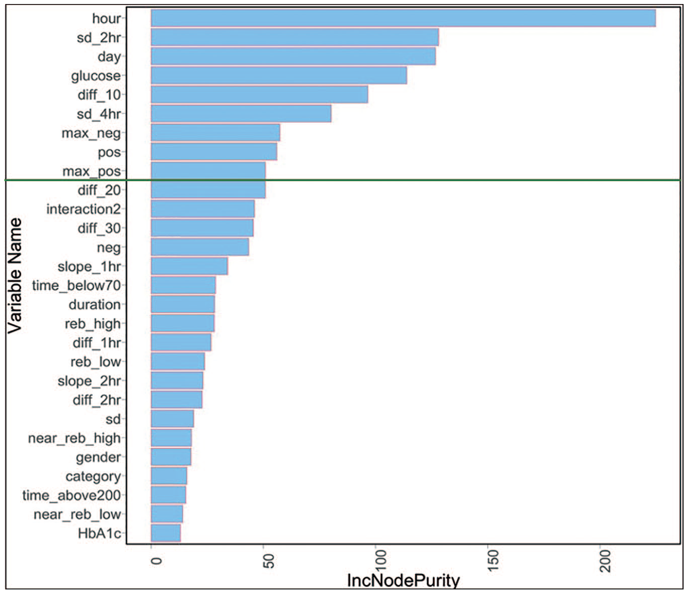
Variable importance plot for random forests.

Seventy percent training and 30% testing partition were randomly repeated 10 times and performance results averaged across these 10 replications to generate robust estimates for sensitivity and specificity. VIP optimized model was used for developing different models for daytime and nighttime risk as well as for evaluating effects of insulin and carbohydrate.

Results

Feature Selection

Figure 4 provides misclassification error curve for the number of variables used in the LR model. The two vertical dashed lines represent λ_min (that corresponds to minimal cross-validation misclassification rate) and λ_1se (that corresponds to model with error falling within one standard deviation of the minimum). The upper x-axis represents the number of features in model for the corresponding λ, with λ_1se being used to select 21 significant features for the final LR model.

Figure 4.

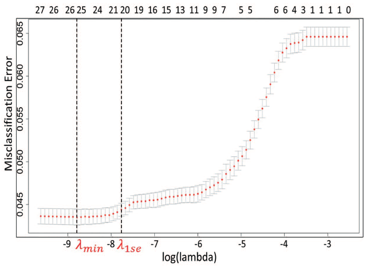
Cross-validation error rate in LASSO.

For RF, as shown in Fig. 5, the misclassification rate increases significantly when the number of variables is less than nine important features. Thus, the top nine significant variables from the VIP are selected for the final RF model (Fig. 3). Table 5 provides a summary of features selected for LR and RF models.

Figure 5.

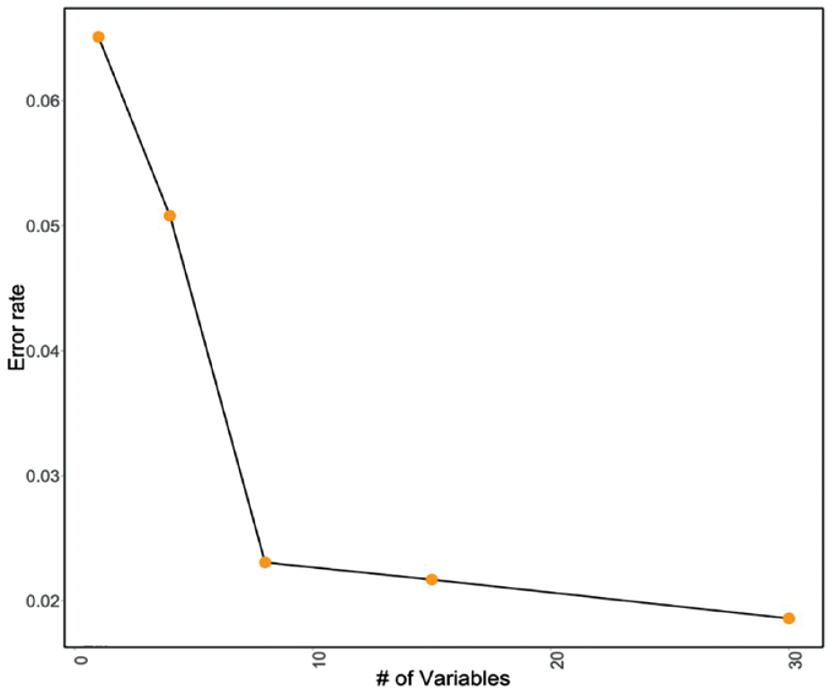
RF out-of-bag misclassification rates.

Table 5.

Model Configurations.

Method	Features
LR with all features	All features in Table 1
RF with all features	All features in Table 2
LR with LASSO selected features	glucose, hour, day, slope_2hr, diff_1hr, diff_10, sd, sd_2hr, category, duration, gender, HbA1c, near_reb_high, time_below70, time_above200, glucose_sq, sd_4hr, pos, neg, max_pos, max_neg
RF with VIP selected features	hour, sd_2hr, day, glucose, diff_10, sd_4hr, max_neg, pos, max_pos
RF with insulin and carb data	RF with VIF selected features, and insulin and carb on board

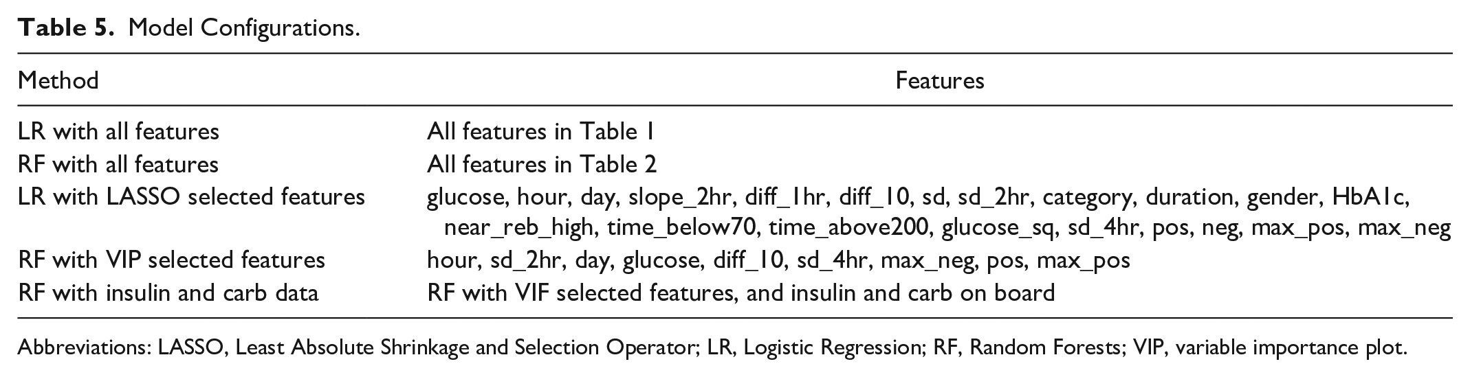
Abbreviations: LASSO, Least Absolute Shrinkage and Selection Operator; LR, Logistic Regression; RF, Random Forests; VIP, variable importance plot.

Classification Performance

Table 3 summarizes model performance. Sensitivity dropped only about 1% point for both the LASSO and VIP selected features when compared with the full model. This is even more significant for RF models as only 9 out of the total 26 features are used in the final model. Our predictions uniformly remained above the 90% mark in identifying hypoglycemic events while only reporting 8%-10% false positives, be it for 0-15-minute or 45-60-minute prediction intervals. The sensitivity drops from 91% for RF to 58% for LR in 45-60-minute window, giving RF models a significant advantage for longer prediction horizons. RF models seem to capture the complex nonlinear relationships influencing hypoglycemia risk much better for different prediction horizons. Figure 6 gives summary of the confusion matrices of VIP Optimized RF for all the prediction horizons. Since this is a rare event classification problem, we set an appropriate threshold level for optimizing the trade-off between sensitivity and specificity through the Receiver Operating Characteristic curves (Fig. 7).

Figure 6.

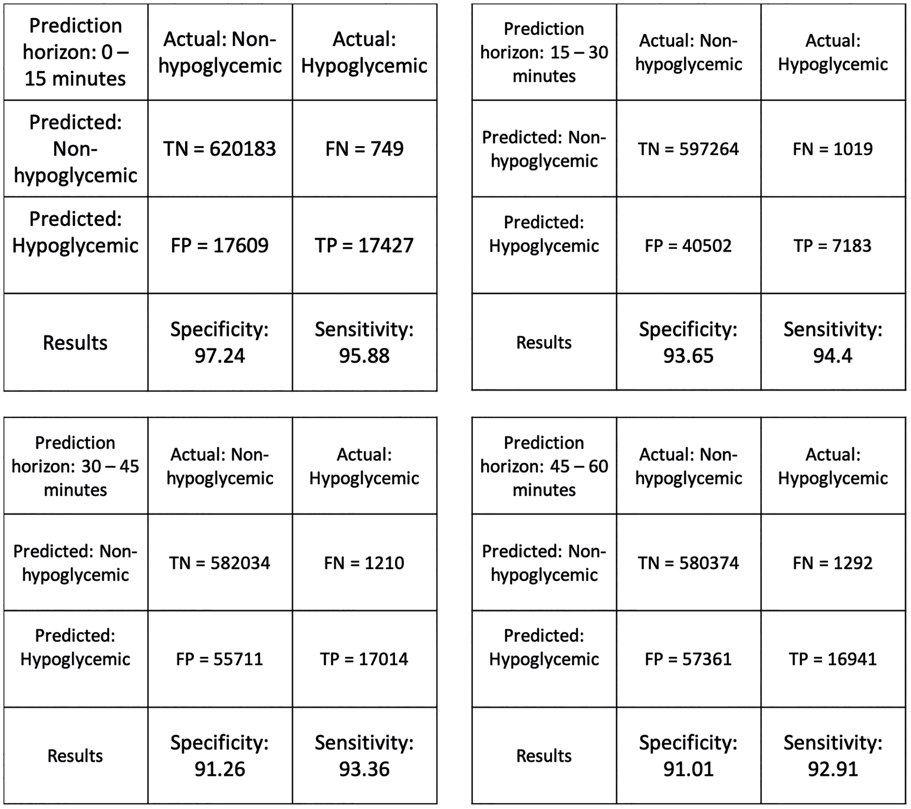
Confusion matrices for prediction horizons: (a) 0-15 minutes, (b) 15-30 minutes, (c) 30-45 minutes, and (d) 45-60 minutes.

Figure 7.

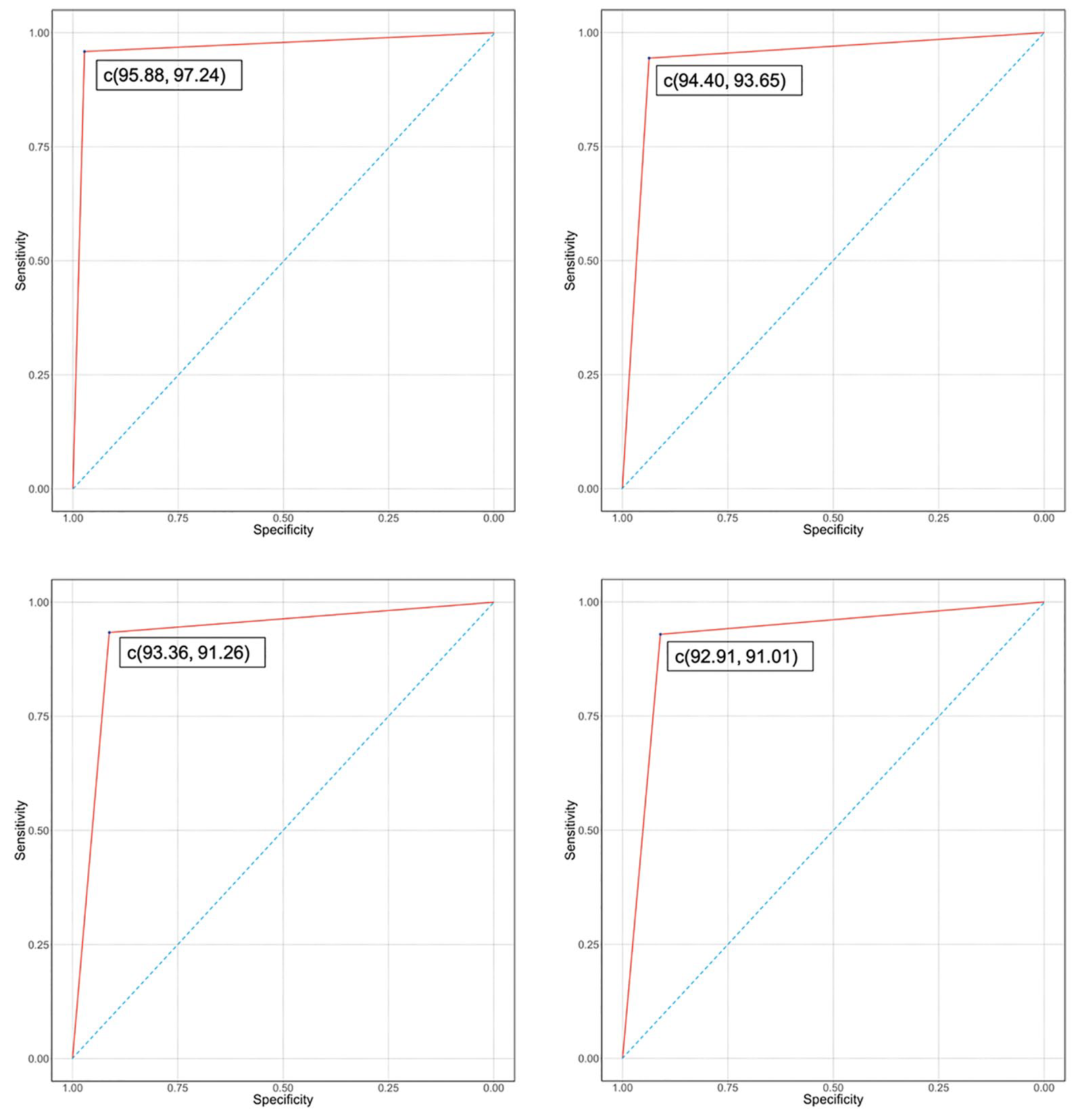
ROC curves for prediction horizons: (Upper left) 0-15 minutes, (Upper right) 15-30 minutes, (Lower left) 30-45 minutes, and (Lower right) 45-60 minutes.

Table 3 also includes performance metrics when separate models were considered for day and night hypoglycemia risk (RF-Day and RF-Night). Night models had a consistent 5% advantage over to daytime predictions, or when considering single model for day or night. We also present a visual comparison of performance of different classifiers (Fig. 8A, B).

Figure 8.

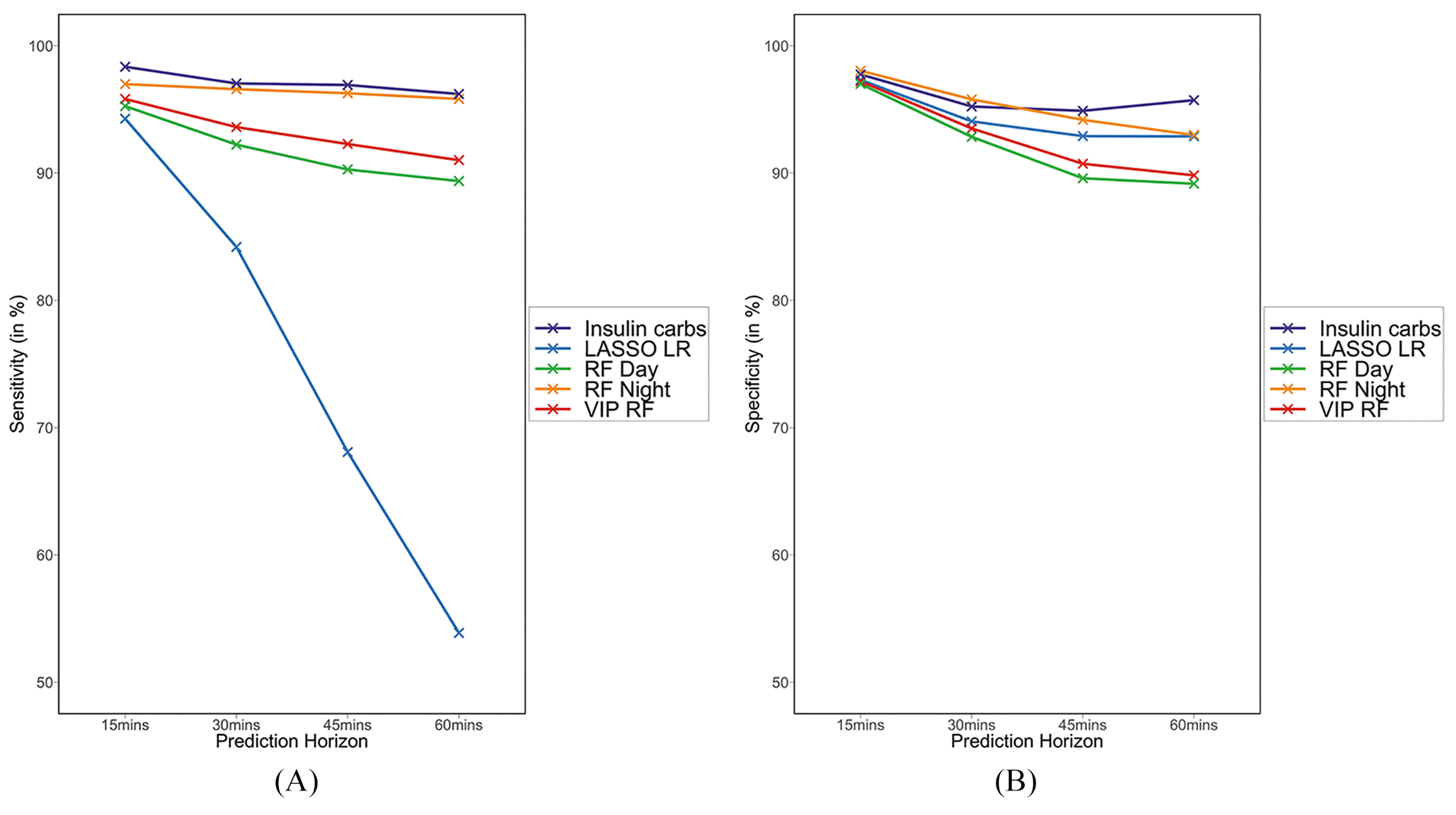
(A) Comparison of sensitivity for various models at different prediction horizons. (B) Comparison of specificity for various models at different prediction horizons.

Discussion

The main contributions of our work to address the challenge of hypoglycemic risk prediction are:

(1) A comprehensive feature-engineering process to identify the features influencing future hypoglycemia risk. We extracted short-term (less than one hour), medium-term (one to four hours), and long-term (more than four hours) patterns from the CGM signal, as well as demographic, contextual, interaction, and nonlinear features and use these features to improve the performance of prediction model.

(2) Ideal set of features for prediction performance and ease of deployment were identified.

(3) Hypoglycemic risk prediction within an interval (0-15, 15-30, 30-45, and 45-60 minutes). In contrast, existing approaches focus on prediction at a discrete point in time (30 and 60 minutes).

(4) Significant improvement in sensitivity and specificity of predictions (Table 6).

Table 6.

Literature Comparison.

Method references	Required input variables	Prediction horizon	Sensitivity (%)	Specificity (%)
Subject-specific recursive time-series models²³	CGM, physical activity, IOB	27.7 ± 5.32	89	78
Extreme Learning Machines (ELM) and Regularized ELM (RELM)⁵²	CGM	30	95.4	-
AR models with exogenous variables⁴⁴	CGM, IOB, CHO intake	30	75	98
Multiple ML algorithms¹⁰	CGM	30	95	-
Recurrent neural networks⁵³	CGM	30	90.87	-
Optimal estimation—Kalman filter^34,54	CGM	1-30	91	79
Our research “Within Time t”	CGM	30/60	93.61/91.01	93.50/89.82
Our research “Within Time t”	CGM, IOB, COB	30/60	97.04/96.21	95.23/95.73
Our research “at Time t”	CGM	30/60	90.93/86.28	93.65/93.07

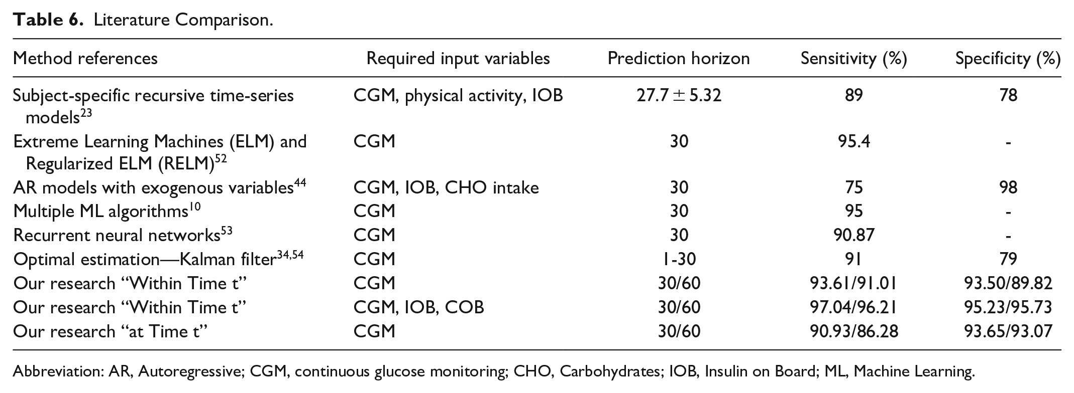
Abbreviation: AR, Autoregressive; CGM, continuous glucose monitoring; CHO, Carbohydrates; IOB, Insulin on Board; ML, Machine Learning.

Insights and Observations

RF seem to be able to capture the complex, nonlinear patterns affecting hypoglycemia better than LR. As evident from the results, we were able to accurately predict true hypoglycemic instances not only for shorter durations but also for longer prediction horizons up to 60 minutes with more than 90% accuracy. This has clinical significance because the additional time may provide more flexibility for the patient to respond. The VIP optimized RF model was able to achieve high performance with only 9 features compared to 21 needed for LR (Table 5). A majority (seven out of nine) of the features used in the VIP optimized RF model are short (less than one hour) and medium (one to four hours) time range, while the other two were contextual features representing day of the week and hour of the day. This is important since it implies that the prediction model can be implemented for new patients without having to collect large amount of data. Based on this insight, the RF-based prediction model will be deployed in the pilot.

We extended the VIP optimized RF model to develop separate models for daytime and nighttime risk with the selected set of nine features. The VIP optimized RF is trained independently on daytime and nighttime data. Developing a separate prediction model for night resulted in significant performance improvement in detecting nocturnal hypoglycemia. While this may not be surprising, due to reduced influences of physical activity and food intake at night, the result is clinically relevant to address the serious consequences of nocturnal hypoglycemia.¹⁴ While the relative ranking of the important features are changed, the list of the important features for the nighttime prediction model are mostly same as whole day model, except that diff-20, time-below-70, and diff-30 replaced sd-4hr, pos, max-pos in the shortlist.

Finally, insulin and carbohydrate data resulted in performance improvement for 30- to 60-minute predictions. Currently, insulin and carbohydrate data are not available in real time from insulin pumps. This study highlights the need to have these data available in real time for facilitating longer horizon hypoglycemic predictions.

Performance Comparison

Most approaches in the literature use raw CGM and supplemental data streams and rely on the algorithm for achieving good model performance. Classical time-series-based approaches as well as optimal estimation theory models like Kalman filter offer the advantages of having a simplistic structure and are more interpretable. However, these methods have significant prediction errors and a very limited forecasting window.⁵⁵ On the other hand, sequence-based neural networks dynamically capture complex patterns from the signal and provide more predictive power, but it comes at the cost of model complexity and require large amounts of processed data. In contrast, our approach relies on a rich set of features that capture the patterns and events influencing the hypoglycemia risk. We were able to achieve exceptional predictive performance using only nine features for RF. These nine features are derived from CGM observations in a four-hour window and are computationally simple. Therefore, our approach provides a simplistic structure of classical parameter-based models while deriving the predictive strength of dynamic models by capturing complex patterns through easy-to-calculate features. In this way, we derive the advantages of both the approaches while implementing the trained model in a device. The implemented model continuously monitors for hypoglycemia risk by just updating the latest CGM value.

We compare our performance results with literature in Table 6, which summarizes our results for both “at time t” as well as “within time t” approaches for t = 30 and 60 minutes in the last two rows. It can be observed that “at time t” predictions accuracies, especially specificity, are a little lower than “within time t” predictions, but are still good performance results. Comparison of performance results across different studies is complicated due to the differences in the definition of hypoglycemic event.^18,56
-58 We use a threshold of 70 mg/dL to define a hypoglycemic event. Most studies report predictions at a specific time in the future. Predictions within an interval is a contribution of this study. We report results for both interval and specific time-based predictions.

Some studies^12,59
-63 have relied on simulated data or data that have been collected through a controlled study. Such data might not truly capture the variations in glucose levels that a person might experience in normal living conditions. Some studies are based on very limited sample size.^13,64 Use of a large sample size under normal living conditions will ensure generalizability of the results. To our knowledge, the sample size used in this study is one of the most comprehensive datasets used in hypoglycemia prediction studies.

On the statistical aspect, in rare event classification problems, such as hypoglycemia prediction, it is important to evaluate model performance on specificity as well as sensitivity, since false alarms can be a major drawback. Some studies do not report specificity or report performance metrics using statements that are difficult to compare across studies such as “low false alarm rates of only 1 or 2 per week.”⁶⁰ These metrics are highly dependent on the frequency of hypoglycemic events in the study dataset and make it difficult to compare performance across different datasets.

Differential Effect of Inclusion of Insulin and Carb on Board

The inclusion of insulin and carbohydrate data resulted in incremental performance improvement especially for 30-60-minute predictions, which is consistent with the findings of Zecchin et al.⁴¹

Limitations and Future Work

The insulin and carbohydrate analysis was based on only 19 patients, compared to CGM data on 112 patients. Although the insulin data coverage was stratified by gender and age group to be representative of the overall study population, a larger sample size would have facilitated more generalizable results. The carbohydrates on board in this study is based on patient-estimated carbohydrate intake which can be an unreliable estimate. We only consider insulin data related to food bolus and ignored basal insulin in this study. In the future, we plan to explore analysis of basal insulin as well as timing of bolus insulin relative to carbohydrate intake and exercise. Finally, we plan to build more individualized prediction model where a personalized model complements a generalized prediction algorithm. This will help leverage glucose patterns unique to a specific individual.

Comparison to Currently Available Systems

Basal IQ is a predictive low glucose suspend system that uses a simple algebraic approach to predict glucose levels 30 minutes ahead and suspend basal insulin in the t-slim:X2 pump if glucose values are expected to drop below 80 mg/dL.⁶⁵ The more recently Food and Drug Administration approved Control IQ automated insulin delivery system uses a complex algorithm to project 30-minute glucose values based on the last four readings to modulate insulin pump basal rates.^66,67

The current Dexcom G6 CGM device provides alerts based on user-specified threshold settings. In examining the accuracy of the Dexcom G6 system at a hypoglycemia threshold of 70 mg/dL, the sensitivity and specificity were found to be ~84% and ~85%, respectively, in the 30-minute prediction horizon.⁶⁸ In contrast, our approach is able to achieve much higher sensitivities (~95% and 94%) and specificities (~97% and 95%) for prediction horizons of 0-15 and 15-30 minutes.

Our machine learning-based hypoglycemia prediction model is novel as it relies on a comprehensive feature extraction process to infer glucose patterns and achieve exceptional performance results, which are superior to existing data published in the literature. Also, our model preserves a simplistic structure with an ideal set of features for ease of deployment in a patient-facing mobile application regardless of insulin modality (ie, injections, insulin pump, or even oral agents in the case of type 2 diabetes).

Conclusion

We present an optimized RF model for probabilistic prediction of hypoglycemic risk in type 1 diabetes patients. The final model was derived after careful consideration of linear and nonlinear models using a rich combination of extracted features. An important contribution of this study is the identification of short (less than one hour) and medium (one to four hours) time range features that are ideal for hypoglycemic risk predictions. The VIP optimized model had sensitivity of 94% and 91% for 30 and 60 minutes, respectively. Specificity was 93% for 30 minutes and 90% for 60 minutes prediction horizons. Incremental benefits of including insulin and carbohydrates data were analyzed and found to be useful for 60-minute predictions as a 4%-point increase in prediction performance was observed. Isolating model for nighttime predictions was found to be beneficial to address nocturnal hypoglycemia. The analytical models presented in this article will be implemented in a smartphone application in an upcoming pilot study.

Footnotes

Acknowledgements

This study involves the use of secondary analysis of de-identified data that was not collected specifically for this project and is not human subject research (Texas A&M IRB number 2019-0710).

Declaration of Conflicting Interests

The author(s) declared no potential conflicts of interest with respect to the research, authorship, and/or publication of this article. TAMU and BCM have applied for provisional patent of this technology.

Funding

The author(s) disclosed receipt of the following financial support for the research, authorship, and/or publication of this article: This work was supported by the Real-World Evidence project of FDA grant P50FD006428.

ORCID iD

Madhav Erraguntla

References

Cox

Irvine

Gonder-Frederick

Nowacek

Butterfield

Fear of hypoglycemia: quantification, validation, and utilization. Diabetes Care. 1987;10(5):617-621.

Patton

Dolan

Henry

Powers

SW.

Fear of hypoglycemia in parents of young children with type 1 diabetes mellitus. J Clin Psychol Med Settings. 2008;15(3):252-259.

Van Name

Hilliard

Boyle

, et al. Nighttime is the worst time: parental fear of hypoglycemia in young children with type 1 diabetes. Pediatr Diabetes. 2018;19(1):114-120.

Clarke

Gonder-Frederick

Snyder

Cox

DJ.

Maternal fear of hypoglycemia in their children with insulin dependent diabetes mellitus. J Pediatr Endocrinol Metab. 1998;11(suppl):189-194.

Freckleton

Sharpe

Mullan

The relationship between maternal fear of hypoglycaemia and adherence in children with type-1 diabetes. Int J Behav Med. 2014;21(5):804-810.

Haugstvedt

Wentzel-Larsen

Graue

Søvik

Rokne

Fear of hypoglycaemia in mothers and fathers of children with Type 1 diabetes is associated with poor glycaemic control and parental emotional distress: a population-based study. Diabet Med. 2010;27(1):72-78.

Rodbard

Continuous glucose monitoring: a review of recent studies demonstrating improved glycemic outcomes. Diabetes Technol Ther. 2017;19(S3):S-25-S-37.

Pettus

Edelman

SV.

Recommendations for using real-time continuous glucose monitoring (rtCGM) data for insulin adjustments in type 1 diabetes. J Diabetes Sci Technol. 2017;11(1):138-147.

Bremer

Gough

DA.

Is blood glucose predictable from previous values? A solicitation for data. Diabetes. 1999;48(3):445-451.

10.

Gadaleta

Facchinetti

Grisan

Rossi

Prediction of adverse glycemic events from continuous glucose monitoring signal. IEEE J Biomed Health. 2018;23(2):650-659.

11.

Howsmon

Bequette

BW.

Hypo-and hyperglycemic alarms: devices and algorithms. J Diabetes Sci Technol. 2015;9(5):1126-1137.

12.

Zecchin

Facchinetti

Sparacino

De Nicolao

Cobelli

Neural network incorporating meal information improves accuracy of short-time prediction of glucose concentration. IEEE Trans Biomed Eng. 2012;59(6):1550-1560.

13.

Cichosz

Frystyk

Hejlesen

Tarnow

Fleischer

A novel algorithm for prediction and detection of hypoglycemia based on continuous glucose monitoring and heart rate variability in patients with type 1 diabetes. J Diabetes Sci Technol. 2014;8(4):731-737.

14.

Jensen

Dethlefsen

Vestergaard

Hejlesen

Prediction of nocturnal hypoglycemia from continuous glucose monitoring data in people with type 1 diabetes: a proof-of-concept study. J Diabetes Sci Technol. 2020;11(4):250-256.

15.

Wilson

Tyler

Jacobs

, et al. Patient input for design of a decision support smartphone application for type 1 diabetes [published online ahead of print August 23, 2019]. J Diabetes Sci Technol. 2019. https://doi.org/10.1177/1932296819870231

16.

Jin

Yue

(eds). The prediction model of blood glucose concentration for smart health. 2019 IEEE International Conference on Multimedia & Expo Workshops (ICMEW). Shanghai, China, IEEE; 2019.

17.

Georga

Protopappas

Ardigò

, et al. Multivariate prediction of subcutaneous glucose concentration in type 1 diabetes patients based on support vector regression. IEEE J Biomed Health. 2012;17(1):71-81.

18.

Georga

Protopappas

Ardigò

Polyzos

Fotiadis

DI.

A glucose model based on support vector regression for the prediction of hypoglycemic events under free-living conditions. Diabetes Technol Ther. 2013;15(8):634-643.

19.

Pérez-Gandía

Facchinetti

Sparacino

, et al. Artificial neural network algorithm for online glucose prediction from continuous glucose monitoring. Diabetes Technol Ther. 2010;12(1):81-88.

20.

Zecchin

Facchinetti

Sparacino

Cobelli

Jump neural network for online short-time prediction of blood glucose from continuous monitoring sensors and meal information. Comput Methods Programs Biomed. 2014;113(1):144-152.

21.

Kovatchev

Clarke

Peculiarities of the continuous glucose monitoring data stream and their impact on developing closed-loop control technology. J Diabetes Sci Technol. 2008;2(1):158-163.

22.

ElMoaqet

Tilbury

Ramachandran

SK.

Multi-step ahead predictions for critical levels in physiological time series. IEEE Trans Cybern. 2016;46(7):1704-1714.

23.

Eren-Oruklu

Cinar

Quinn

Hypoglycemia prediction with subject-specific recursive time-series models. J Diabetes Sci Technol. 2010;4(1):25-33.

24.

Eren-Oruklu

Cinar

Quinn

Smith

Estimation of future glucose concentrations with subject-specific recursive linear models. Diabetes Technol Ther. 2009;11(4):243-253.

25.

Gani

Gribok

Ward

Vigersky

Reifman

Universal glucose models for predicting subcutaneous glucose concentration in humans. IEEE Trans Inf Technol Biomed. 2009;14(1):157-165.

26.

Sparacino

Zanderigo

Corazza

Maran

Facchinetti

Cobelli

Glucose concentration can be predicted ahead in time from continuous glucose monitoring sensor time-series. IEEE Trans Biomed Eng. 2007;54(5):931-937.

27.

Wang

A novel adaptive-weighted-average framework for blood glucose prediction. Diabetes Technol Ther. 2013;15(10):792-801.

28.

Bequette

BW.

Continuous glucose monitoring: real-time algorithms for calibration, filtering, and alarms. J Diabetes Sci Technol. 2010;4(2):404-418.

29.

Bequette

Cameron

Buckingham

Maahs

Lum

Overnight hypoglycemia and hyperglycemia mitigation for individuals with type 1 diabetes: how risks can be reduced. IEEE Control Systems Magazine. 2018;38(1):125-134.

30.

Cameron

Wilson

Buckingham

, et al. Inpatient studies of a Kalman-filter-based predictive pump shutoff algorithm. J Diabetes Sci Technol. 2012;6(5):1142-1147.

31.

Hughes

Patek

Breton

Kovatchev

BP.

Hypoglycemia prevention via pump attenuation and red-yellow-green “traffic” lights using continuous glucose monitoring and insulin pump data. J Diabetes Sci Technol. 2010;4(5):1146-1155.

32.

Messer

Calhoun

Buckingham

, et al. In-home nighttime predictive low glucose suspend experience in children and adults with type 1 diabetes. Pediatr Diabetes. 2017;18(5):332-339.

33.

Palerm

Bequette

BW.

Hypoglycemia detection and prediction using continuous glucose monitoring—a study on hypoglycemic clamp data. J Diabetes Sci Technol. 2007;1(5):624-629.

34.

Palerm

Willis

Desemone

Bequette

BW.

Hypoglycemia prediction and detection using optimal estimation. Diabetes Technol Ther. 2005;7(1):3-14.

35.

Sankaranarayanan

Kumar

Cameron

Bequette

Fainekos

Maahs

DM.

Model-based falsification of an artificial pancreas control system. ACM SIGBED Rev. 2017;14(2):24-33.

36.

Turksoy

Bayrak

Quinn

Littlejohn

Rollins

Cinar

Hypoglycemia early alarm systems based on multivariable models. Ind Eng Chem Res. 2013;52(35):12329-12336.

37.

Contreras

Oviedo

Vettoretti

Visentin

Vehí

Personalized blood glucose prediction: a hybrid approach using grammatical evolution and physiological models. PLoS One. 2017;12(11):e0187754.

38.

Herrero

Bondia

Giménez

Oliver

Georgiou

Automatic adaptation of basal insulin using sensor-augmented pump therapy. J Diabetes Sci Technol. 2018;12(2):282-294.

39.

Hovorka

Canonico

Chassin

, et al. Nonlinear model predictive control of glucose concentration in subjects with type 1 diabetes. Physiol Meas. 2004;25(4):905.

40.

Walsh

Roberts

Bailey

Heinemann

Bolus advisors: sources of error, targets for improvement. J Diabetes Sci Technol. 2018;12(1):190-198.

41.

Zecchin

Facchinetti

Sparacino

Cobelli

How much is short-term glucose prediction in type 1 diabetes improved by adding insulin delivery and meal content information to CGM data? A proof-of-concept study. J Diabetes Sci Technol. 2016;10(5):1149-1160.

42.

Oviedo

Vehí

Calm

Armengol

A review of personalized blood glucose prediction strategies for T1DM patients. Int J Numer Method Biomed Eng. 2017;33(6):e2833.

43.

Yang

Shi

Xie

An ARIMA model with adaptive orders for predicting blood glucose concentrations and hypoglycemia. IEEE J Biomed Health. 2018;23(3):1251-1260.

44.

Zisser

Robinson

Bevier

, et al. Bolus calculator: a review of four “smart” insulin pumps. Diabetes Technol Ther. 2008;10(6):441-444.

45.

Yeager

. What to eat and drink during rides of every length. Bicycling. Hearst Magazine Media, Inc; February 12, 2019 [Online]. https://www.bicycling.com/training/a20011394/how-to-fuel-on-rides-of-every-length/. Accessed February 30, 2019.

46.

Leiter

Yoon

K-H

Arias

, et al. Canagliflozin provides durable glycemic improvements and body weight reduction over 104 weeks versus glimepiride in patients with type 2 diabetes on metformin: a randomized, double-blind, phase 3 study. Diabetes Care. 2015;38(3):355-364.

47.

Ratner

RE.

Hypoglycemia: new definitions and regulatory implications. Diabetes Technol Ther. 2018;20(S2):S2-50-S2-3.

48.

Erraguntla

Zapletal

Lawley

Framework for infectious disease analysis: a comprehensive and integrative multi-modeling approach to disease prediction and management. Health Informatics J. 2019;25(4):1170-1187.

49.

Sultana

Erraguntla

Kum

H-C

Lawley

Post-acute care referral in United States of America: a multiregional study of factors associated with referral destination in a cohort of patients with coronary artery bypass graft or valve replacement. BMC Med Inform Decis Mak. 2019;19(1):223.

50.

Abbas

Alic

Erraguntla

, et al. Predicting long-term type 2 diabetes with support vector machine using oral glucose tolerance test. PLoS One. 2019;14(12):1-12.

51.

Breiman

Random forests. Machine Learn. 2001;45(1):5-32.

52.

Wang

(eds). Hypoglycemia prediction using extreme learning machine (ELM) and regularized ELM. 2013 25th Chinese Control and Decision Conference (CCDC). Guiyang, China, IEE; 2013.

53.

Mosquera-Lopez

Dodier

Tyler

Resalat

Jacobs

Leveraging a big dataset to develop a recurrent neural network to predict adverse glycemic events in type 1 diabetes [published online ahead of print April 17, 2019]. IEEE J Biomed Health. 2019. doi: 10.1109/JBHI.2019.2911701.

54.

Hamdi

Ali

Di Costanzo

Fnaiech

Moreau

Ginoux

J-M.

Accurate prediction of continuous blood glucose based on support vector regression and differential evolution algorithm. Biocybern Biomed Eng. 2018;38(2):362-372.

55.

Aliberti

Pupillo

Terna

, et al. A multi-patient data-driven approach to blood glucose prediction. IEEE Access. 2019;7:69311-69325.

56.

Cameron

Niemeyer

Gundy-Burlet

Buckingham

Statistical hypoglycemia prediction. J Diabetes Sci Technol. 2008;2(4):612-621.

57.

Jensen

Christensen

Tarnow

Seto

Dencker Johansen

Hejlesen

OK.

Real-time hypoglycemia detection from continuous glucose monitoring data of subjects with type 1 diabetes. Diabetes Technol Ther. 2013;15(7):538-543.

58.

Jensen

Mahmoudi

Christensen

, et al. Evaluation of an algorithm for retrospective hypoglycemia detection using professional continuous glucose monitoring data. J Diabetes Sci Technol. 2014;8(1):117-122.

59.

Cappon

Vettoretti

Marturano

Facchinetti

Sparacino

A neural-network-based approach to personalize insulin bolus calculation using continuous glucose monitoring. J Diabetes Sci Technol. 2018;12(2):265-272.

60.

Dassau

Cameron

Lee

, et al. Real-time hypoglycemia prediction suite using continuous glucose monitoring: a safety net for the artificial pancreas. Diabetes Care. 2010;33(6):1249-1254.

61.

Liu

Zhu

Herrero

Georgiou

GluNet: a deep learning framework for accurate glucose forecasting. IEEE J Biomed Health. 2020;24(2):414-423.

62.

Mahmoudi

Jensen

Dencker Johansen

, et al. Accuracy evaluation of a new real-time continuous glucose monitoring algorithm in hypoglycemia. Diabetes Technol Ther. 2014;16(10):667-678.

63.

Reddy

Resalat

Wilson

Castle

El Youssef

Jacobs

PG.

Prediction of hypoglycemia during aerobic exercise in adults with type 1 diabetes. J Diabetes Sci Technol. 2019;13(5):919-927.

64.

Montaser

Diez

Rossetti

Rashid

Cinar

Bondia

Seasonal local models for glucose prediction in type 1 diabetes [published online ahead of print November 29, 2019]. IEEE J Biomed Health. 2019. doi: 10.1109/JBHI.2019.2956704.

65.

Forlenza

Buckingham

, et al. Predictive low-glucose suspend reduces hypoglycemia in adults, adolescents, and children with type 1 diabetes in an at-home randomized crossover study: results of the PROLOG trial. Diabetes Care. 2018;41(10):2155-2161.

66.

Brown

Kovatchev

Raghinaru

, et al. Six-month randomized, multicenter trial of closed-loop control in type 1 diabetes. N Engl J Med. 2019;381(18):1707-1717.

67.

Diabetes

. Tandem’s Control IQ Explained. Tandem Diabetes Care Inc. https://www.tandemdiabetes.com/providers/products/basal-iq. Accessed February 20, 2020.

68.

Wadwa

Laffel

Shah

Garg

SK.

Accuracy of a factory-calibrated, real-time continuous glucose monitoring system during 10 days of use in youth and adults with diabetes. Diabetes Technol Ther. 2018;20(6):395-402.

Feature-Based Machine Learning Model for Real-Time Hypoglycemia Prediction

Abstract

Background:

Methods:

Results:

Conclusions:

Keywords

Introduction

Methods

Materials

Feature Extraction

Machine Learning Algorithms/Methodologies

Hypoglycemic Prediction Window

Feature Selection and Classifier Evaluation

Results

Feature Selection

Classification Performance

Discussion

Insights and Observations

Performance Comparison

Differential Effect of Inclusion of Insulin and Carb on Board

Limitations and Future Work

Comparison to Currently Available Systems

Conclusion

Footnotes

Acknowledgements

Declaration of Conflicting Interests

Funding

ORCID iD

References