Sage Journals: Discover world-class research

Abstract

Background:

This study investigates blood glucose (BG) measurement interpolation techniques to represent intermediate BG dynamics, and the effect resampling of retrospective BG data has on key glycemic control (GC) performance results. GC protocols in the ICU have varying BG measurement intervals ranging from 0.5 to 4 hours. Sparse data pose problems, particularly in comparing GC performance or model fitting, and thus interpolation is required.

Methods:

Retrospective data from SPRINT in Christchurch Hospital Intensive Care Unit (ICU) (2005-2007) were used to analyze several interpolation techniques. Piecewise linear, spline, and cubic interpolation functions, which force interpolation through measured data, as well as 1st and 2nd Order B-spline basis functions, are used to identify the interpolated trace. Dense data were thinned to increase sparsity and obtain measurements (Hidden Measurements) for comparison after interpolation. Performance is assessed based on error in capturing hidden measurements. Finally, the effect of minutely versus hourly sampling of the interpolated trace on key GC performance statistics was investigated using retrospective data received from STAR GC in Christchurch Hospital ICU, New Zealand (2011-2015).

Results:

All of the piecewise functions performed considerably better than the fitted interpolation functions. Linear piecewise interpolation performed the best having a mean RMSE 0.39 mmol/L, within 2 standard deviations of the BG sensor error. Minutely sampled BG resulted in significantly different key GC performance values when compared to raw sparse BG measurements.

Conclusion:

Linear piecewise interpolation provides the best estimate of intermediate BG dynamics and all analyses comparing GC protocol performance should use minutely linearly interpolated BG data.

Keywords

glycemic control retrospective BG interpretation point-of-care blood glucose intensive care

Providing glycemic control (GC) in any situation, whether it be in individuals with diabetes or stress heighted intensive care unit (ICU) patients, is commonly done via point-of-care blood glucose (BG) meter measurements. In addition, to lower workload and disturbance the frequency of these measures is often kept to a minimum.^1-3 Approximately every 4 to 8 hours is recommended in individuals with diabetes³ and 1 to 4 hours in stress heighted ICU patients.^4,5 As a result, the data collected are sparse and the intermediate BG dynamics unknown. Therefore, interpolation is required to approximate the intermediate dynamics for GC protocols/models and, retrospectively, to fairly assess GC performance.

In particular, many insulin-glucose models and/or model-based GC protocols use parameter identification techniques that require an approximation of the continuous BG dynamics.^6-12 The choice of approximation can significantly skew model fit and “accuracy.” Many models and identification methods use linear interpolation between BG measurements as a first approach.^9,13 However, the accuracy of linear interpolation in comparison to other interpolation techniques has not been assessed.

Similarly, GC protocols in the ICU and many other aspects of diabetes use a range of different BG measurement intervals (eg, 0.5-4 hours in the ICU). These intervals can vary during treatment depending on a patient’s condition,^14-19 compliance,²⁰ or other human factors.²¹ In particular, most ICU GC protocols measure more frequently when patients are out of their targeted band, and less frequently when patients are “stable” and in the targeted band,^14-19 directly skewing raw data performance metrics.

Therefore, the BG information recorded by each GC protocol has varying degrees of sparsity, with raw BG measurements commonly being denser in areas of poor control. This variability and skewness of the raw BG measurements make fair assessment and comparison of GC protocol performance difficult, particularly when one key ICU GC performance criteria is percentage of time within, above, and below a targeted BG range.²² Thus, metrics calculated from raw data cannot provide a fair comparison nor a fair assessment of performance.

A common method to improve assessment fairness is to interpolate between BG measurements and sample the interpolated trace.^14,17-19 However, the best interpolation technique and sample rate is still unknown. This study seeks to answer both of these questions.

Methods

Patient Data

Patient data from patients treated with Specialized Relative Insulin-Nutrition Tables (SPRINT) and Stochastic TARgeted (STAR) in Christchurch Hospital ICU, New Zealand (NZ) between 2005-2016 are used.^14,19,23 SPRINT is a paper-based ICU GC protocol that used 1- to 2-hour measurement intervals and allows the time of BG measurements to be recorded to an hourly resolution.¹⁴ In contrast, STAR is a tablet-based ICU GC protocol using 1- to 3-hour measurement intervals and allows the time of BG measurements to be recorded to a resolution in minutes.^19,23 The Upper South Regional Ethics Committee, NZ granted approval for the retrospective audit, analysis and publication of the Christchurch Hospital patient data.

To answer the first question and assess which interpolation technique best captures the intermediate BG dynamics, a representative sample of the densely measured SPRINT cohort data is used.¹⁴

To answer the second question, the effect of sampling rate (minutely vs hourly and raw) on GC performance statistics is assessed using the more sparsely measured STAR cohort data.

Question 1: Interpolation Techniques

Five interpolation techniques are investigated, separated into 2 types of interpolation:

Piecewise interpolation: The interpolated trace goes through all of the measurement points.

Fitted interpolation: The interpolated trace is a combination of basis function (BF), best fit to the measured data points, as a whole, but can miss any individual point.

Piecewise Interpolation

Three piecewise interpolation techniques are investigated: linear, spline, and cubic. Examples are shown in Figure 1, and they are defined as follows:

Linear interpolation: Data between BG measurements are assumed to be a linear line. Thus, continuous BG data are represented by a piecewise 1st order polynomial.

Spline interpolation: Data between BG measurements are assumed to follow a spline using not-a-knot end conditions, continuous in both 1st and 2nd derivatives. Thus, continuous BG data are represented by cubic interpolation of the spline.

Cubic interpolation: Data between BG measurements are assumed to be a cubic relationship, continuous in only the 1st derivative. Thus, continuous BG data are represented by a piecewise cubic polynomial.

Figure 1.

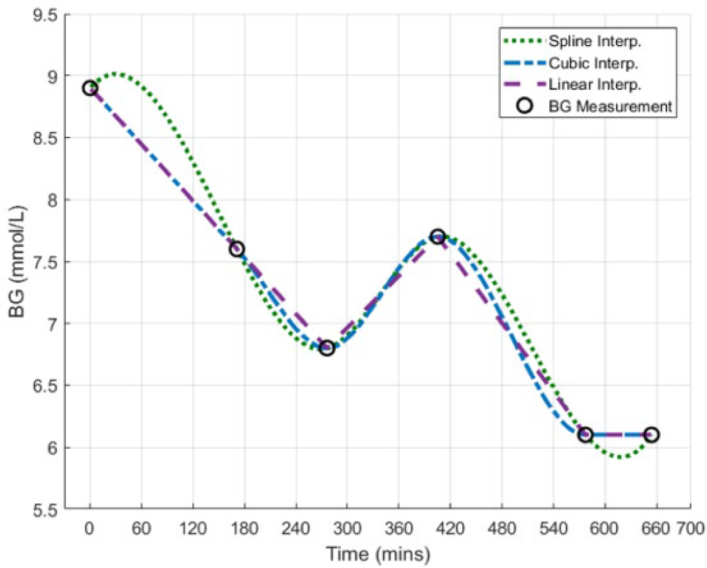
Example of the piecewise interpolation techniques being investigated.

Fitted Interpolation

Two fitted interpolation techniques are investigated, each using 1st and 2nd Order B-spline BF fitting. Note, zeroth Order B-spline BFs were not used as constant stepwise dynamics are not representative of physiologically observed BG dynamics, despite their ease of use mathematically. In addition, 3rd Order and higher B-spline BFs were not used as they add further complexity and heavily restrict BG dynamics. Fitted interpolation is used to incorporate an approximation of the measurement error, and restrict over fitting rapid changes in the interpolated BG trace due to measurement error and outliers. BF widths were varied to investigate the best fit with these criteria.

The interpolated BG trace, G(t), is identified as the linear combination of BFs, Φn(t), minimizing the error between the identified and clinically measured BG:

[\begin{matrix} \begin{matrix} Φ_{1} (t_{1}) & Φ_{2} (t_{1}) \\ Φ_{1} (t_{2}) & Φ_{2} (t_{2}) \end{matrix} & \begin{matrix} \dots & Φ_{n} (t_{1}) \\ \dots & Φ_{n} (t_{2}) \end{matrix} \\ \begin{matrix} ⋮ & ⋮ \\ Φ_{1} (t_{m}) & Φ_{2} (t_{m}) \end{matrix} & \begin{matrix} ⋱ & ⋮ \\ \dots & Φ_{n} (t_{m}) \end{matrix} \end{matrix}] [\begin{matrix} \begin{matrix} γ_{1} \\ γ_{2} \end{matrix} \\ \begin{matrix} ⋮ \\ γ_{n} \end{matrix} \end{matrix}] = [\begin{matrix} \begin{matrix} B G_{m e a s} (t_{1}) \\ B G_{m e a s} (t_{2}) \end{matrix} \\ \begin{matrix} ⋮ \\ B G_{m e a s} (t_{m}) \end{matrix} \end{matrix}]

[\begin{matrix} \begin{matrix} Φ_{1} (t) & Φ_{2} (t) \end{matrix} & \begin{matrix} \dots & Φ_{n} (t) \end{matrix} \end{matrix}] [\begin{matrix} \begin{matrix} γ_{1} \\ γ_{2} \end{matrix} \\ \begin{matrix} ⋮ \\ γ_{n} \end{matrix} \end{matrix}] = G_{i n t e r p} (t)

$\begin{array}{l} W h e r e : Φ_{n} = b a s i s f u n c t i o n n, γ_{n} = f i t t e d b a s i s f u n c t i o n \\ c o e f f i e c e n t n, \\ B G_{m e a s} (t_{m}) = B G m e a s u r e m e n t a t t i m e t_{m}, \\ n = n u m b e r o f b a s i s f u n c t i o n s, \\ m = n u m b e r o f B G m e a s u r e m e n t s, \\ G_{i n t e r p} (t) = i n t e r p o l a t e d B G t r a c e \end{array}$

1st Order B-spline BFs: The BG interpolation trace is made from a linear combination of 1st Order B-spline BFs. 1st Order B-spline BFs are based on the piecewise function defined in De Boor.²⁴ When k = 1 (1st Order BF) the equation simplifies to:

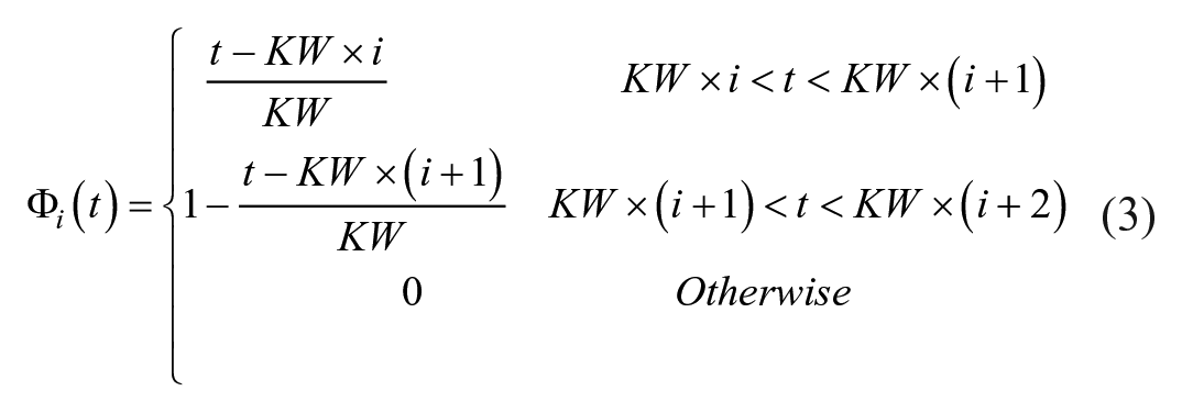
Φ_{i} (t) = {\begin{matrix} \begin{matrix} \frac{t - K W \times i}{K W} & K W \times i < t < K W \times (i + 1) \end{matrix} \\ \begin{matrix} 1 - \frac{t - K W \times (i + 1)}{K W} & K W \times (i + 1) < t < K W \times (i + 2) \end{matrix} \\ \begin{matrix} 0 & O t h e r w i s e \end{matrix} \end{matrix}

$\begin{array}{l} W h e r e : Φ_{i} = b a s i s f u n c t i o n i, K W = k n o t w i d t h, \\ i = b a s i s f u n c t i o n n u m b e r \end{array}$

2nd Order B-spline BFs: The BG interpolation trace is made from a linear combination of 2nd Order B-spline BFs, again using the piecewise function defined in De Boor.²⁴ When k = 2 (2nd Order BF) the equation simplifies to:

Φ_{i} (t) = {\begin{matrix} \frac{{(t - K W \times i)}^{2}}{2 \times K W^{2}} K W \times i < t < K W \times (i + 1) \\ \begin{array}{l} \frac{- 1}{K W^{2}} {(K W \times (i + \frac{3}{2}) - t)}^{2} + \frac{3}{4} K W \times (i + 1) < t < K W \times (i + 2) \\ \begin{array}{l} \frac{{(K W \times (i + 3) - t)}^{2}}{2 \times K W^{2}} K W \times (i + 2) < t < K W \times (i + 3) \\ 0 O t h e r w i s e \end{array} \end{array} \end{matrix}

\sum_{i = 1}^{n} Φ_{i} (t) = 1 \forall t

\begin{array}{l} W h e r e : Φ_{i} = b a s i s f u n c t i o n i, K W = k n o t w i d t h, \\ i = b a s i s f u n c t i o n n u m b e r, n = n u m b e r \\ o f b a s i s f u n c t i o n s . \end{array}

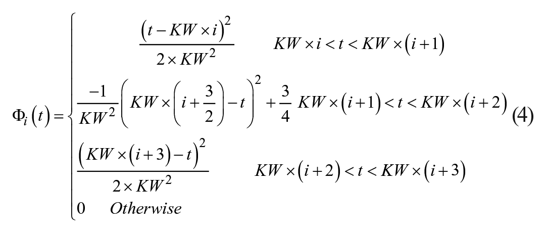
The B-spline BFs are in fixed locations, occurring every instance of the chosen knot width (KW), and overlap each other. The inherent property of the B-spline BFs in equation (5) ensures no underlying waveform can be induced into the fitted data and a constant value can also be represented. An illustrative example of the fitted interpolation techniques can be seen in Figure 2. Note, regularization was not used as it results in the solutions of ill posed problems tending toward the regularization order. For example, 1st Order regularization results in ill posed problems tending toward the linear piecewise interpolation solution.

Figure 2.

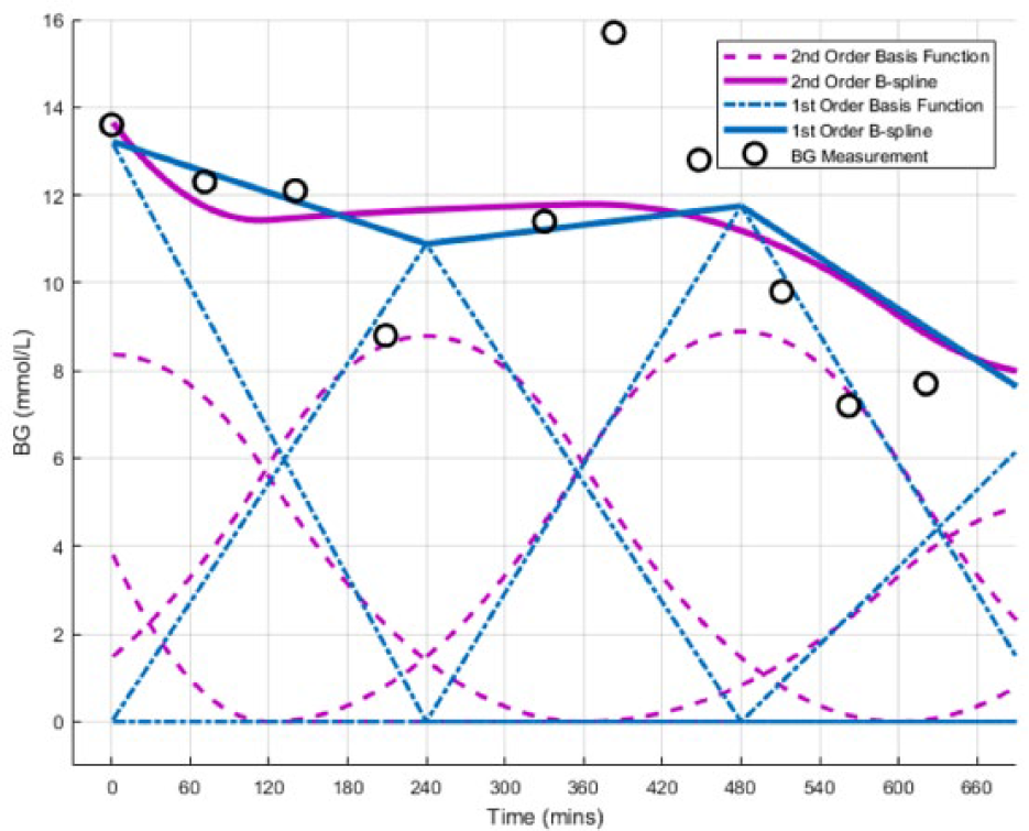
Example of the fitted interpolation techniques (1st and 2nd Order B-spline BFs) being investigated. In this figure the BF KW = 240 minutes.

Interpolation Analysis

To assess which interpolation technique best represents the overall BG dynamics, both the fit to the measured and intermediate BG dynamics needs to be considered. To achieve this goal, a proportion of BG measurements are removed from the dense SPRINT BG measurement sets before interpolation. The removed BG measurements are then compared to the postinterpolation BG estimate for independent validation. Clinical patient BG data were thinned to create 2-, 3-, and 4-hour periods between measurements, similar to what would be expected clinically from STAR¹⁹ and many other protocols.^14-18

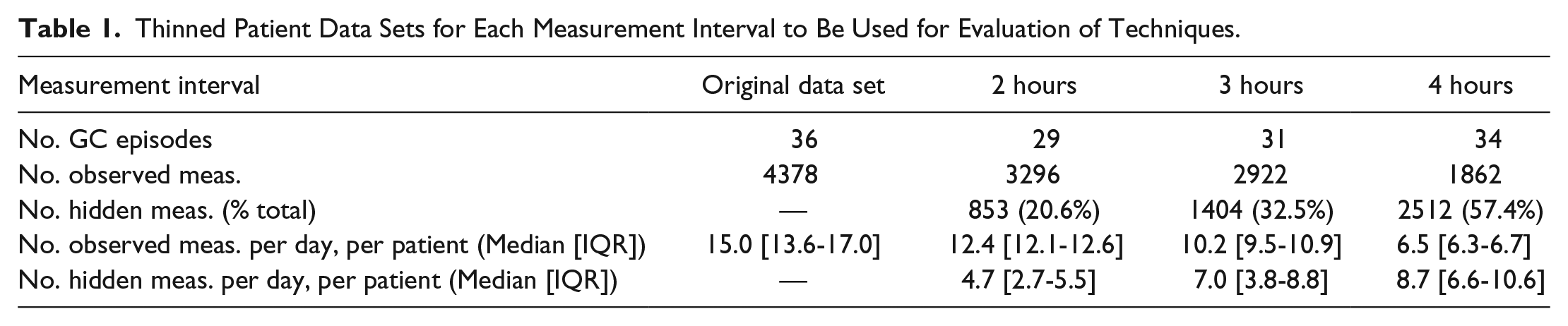
Removed BG measurements are referred to as “hidden” measurements, and the remaining measurements as “observed” measurements. For a BG measurement to be removed it must be able to be removed without causing a gap between the neighboring measurements greater than the measurement period being investigated (2, 3, and 4 hours). Patients who were unable to provide any measurements that met this criterion were excluded from the corresponding thinned data set. An example of this removal process is shown in Figure 3, and Table 1 summarizes the resulting sparse SPRINT BG data.

Figure 3.

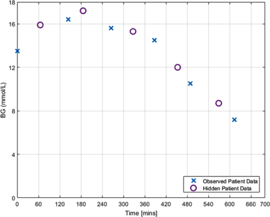
Example of BG measurement removal from patient data to maximize 2-hour BG measurement intervals.

Table 1.

Thinned Patient Data Sets for Each Measurement Interval to Be Used for Evaluation of Techniques.

Measurement interval	Original data set	2 hours	3 hours	4 hours
No. GC episodes	36	29	31	34
No. observed meas.	4378	3296	2922	1862
No. hidden meas. (% total)	—	853 (20.6%)	1404 (32.5%)	2512 (57.4%)
No. observed meas. per day, per patient (Median [IQR])	15.0 [13.6-17.0]	12.4 [12.1-12.6]	10.2 [9.5-10.9]	6.5 [6.3-6.7]
No. hidden meas. per day, per patient (Median [IQR])	—	4.7 [2.7-5.5]	7.0 [3.8-8.8]	8.7 [6.6-10.6]

All interpolation techniques are investigated in regard to goodness of fit of both the observed and hidden data. A range of BF KWs are used for the fitted interpolation techniques, based on equations (3) and (4). Goodness of fit is assessed by using root mean square error (RMSE) between the interpolated trace and the observed and/or hidden measurements. The RMSE for each patient was calculated and the average RMSE from all patients, in the given thinned data set, presented. There is no observed measurement error for the piecewise interpolation techniques as the piecewise functions start and end at the observed measurements, so the hidden measurements are the sole form of validation.

For fitted interpolation, hidden measurement RMSE is expected to be larger than the observed measurement RMSE as observed measurements are used in the identification process. The error for hidden measurements validates the ability of the interpolation technique to capture the intermediate BG dynamics over time intervals relevant to GC protocols. The RMSE for both the observed and hidden measurements are then compared to the error expected from the point-of-care measurement device used in the SPRINT study, Arkray Super-Glucocard™ II glucometer (Arkray, Minneapolis, MN, USA), which has a measurement error standard deviation (SD) ranging from 0.15 to 0.56 mmol/L depending on the BG value.²⁵

Question 2: Sampling Analysis

To assess which sampling rate of the predetermined interpolated BG trace best captures GC performance, key GC performance statistics are compared with various sampling intervals (1 and 60 minute, and original clinical measurement intervals). The commonly used statistics compared are:

BG mean, median, and SD

Percentage of time in the targeted range (4.4-8.0 mmol/L)

Percentage of time BG < 2.2 mmol/L, BG < 4.4 mmol/L, and BG > 10 mmol/L

The percentage of time above, below, or in band statistics can be approximated only with the provided data as the percentage of raw or resampled measurements within a certain range. All sampling of the interpolated BG trace starts from the first BG measurement, thus making it heavily dependent on the interpolation technique used. Nonparametric statistics are used exclusively due to the typically skewed distributions of BG data. P values were computed using the Mann-Whitney rank sum test for all continuous data. P values < .025 are considered statistically significant after Bonferroni correction²⁶ for multiple comparisons.

Results

Question 1: Piecewise Interpolation

Figure 4 shows the cohort RMSE for the hidden measurements for the 3 piecewise interpolation techniques (linear, spline, and cubic), noting observed measurement error is zero as piecewise interpolation forces the trace through the observed measurement data points used. Linear interpolation gave the best estimate of the hidden measurements, having a mean RMSE of 0.39 mmol/L across the 3 intervals investigated. As expected, the longer the measurement interval interpolated, the further the interpolated trace deviated from the hidden BG measurements.

Figure 4.

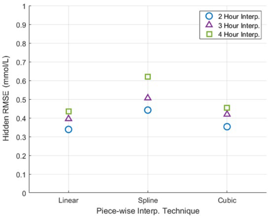
Piecewise interpolation hidden measurement RMSE.

Question 1: Fitted Interpolation

Figures 5 and 6 presents the cohort RMSE, for both hidden and observed measurements of the 1st and 2nd order B-spline BFs, respectively. In both figures, as the KW is increased the observed measurement RMSE is shown to increase, while the hidden measurement RMSE decreases. As expected, the longer the measurement interval interpolated, the further the interpolated trace deviated from the hidden BG measurements and the easier it is for the fitted interpolation technique to capture the slower changing observed BG dynamics.

Figure 5.

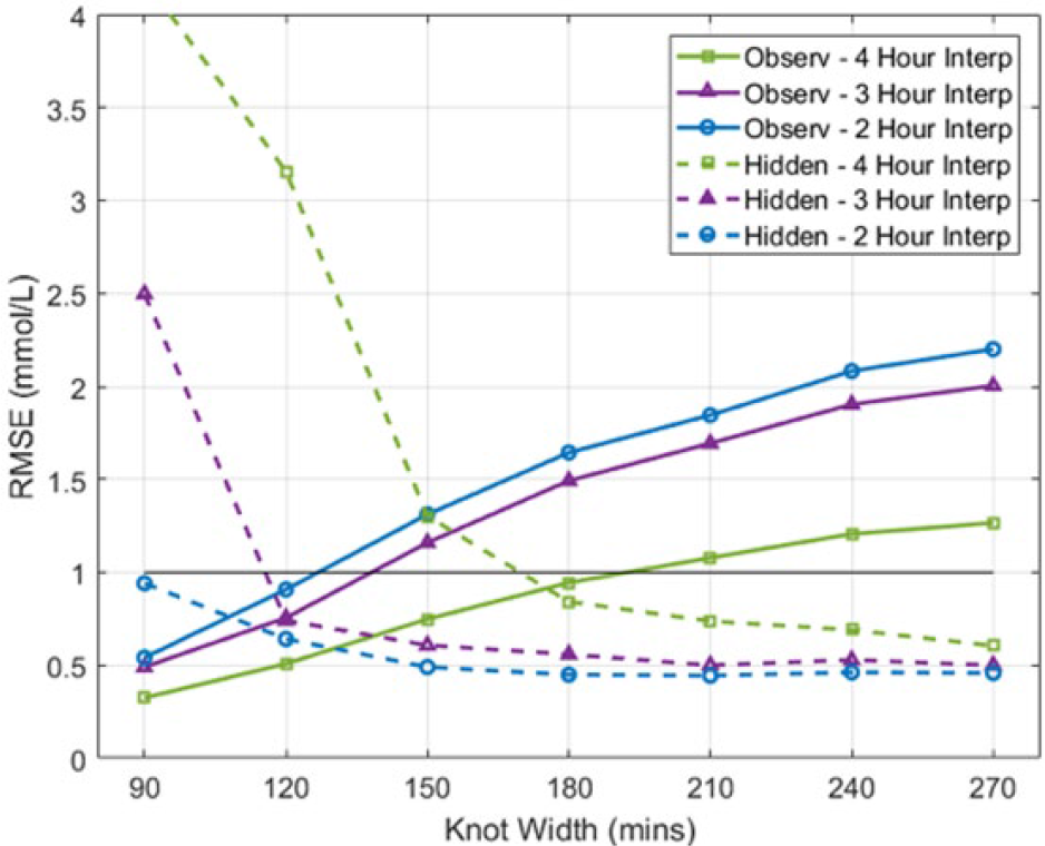
1st Order B-spline BFs fitted interpolation RMSE of observed and hidden measurements. The black line provides reference to the upper limit of Figure 4.

Figure 6.

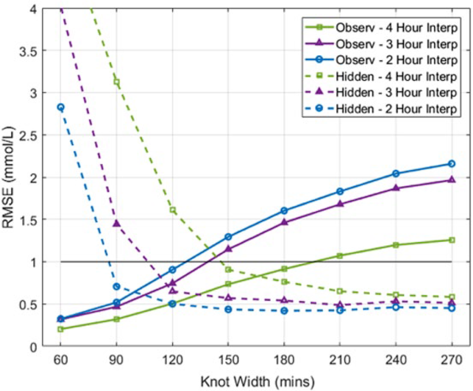
2nd Order B-spline BFs fitted interpolation RMSE of observed and hidden measurements. The black line provides reference to the upper limit of Figure 4.

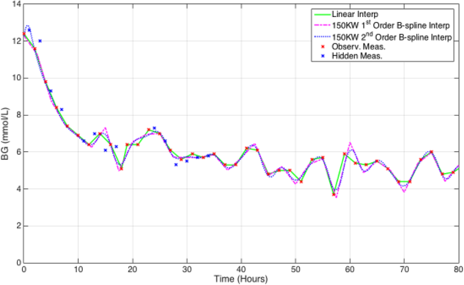
Figure 7 presents a comparison of the fitted interpolation techniques and linear piecewise interpolation. The fitted interpolation can be clearly seen to approximate the BG dynamics as a less erratic, gradually changing mean of the measured BG. Figure 8 shows the influence of increasing the KW used by the B-spline BF, with lower KW providing ill posed, erratic solutions and higher KW providing more of a moving average solution to the BG measures.

Figure 7.

Example of the two fitted interpolation techniques fitted to 2-hour thinned patient data. The linear piecewise interpolation technique is also provided for comparison.

Figure 8.

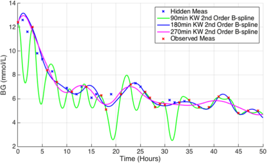
Example of the influence of KW on the fitted interpolation fit.

Question 2: Sampling Interval

The prior analysis shows linear piecewise interpolation provided the best estimate of the intermediate BG dynamics post measurement. Using linear interpolation, the effect of sampling rate on the STAR cohort ICU GC statistics was investigated. Table 2 shows the results are significantly skewed if resampling is not used. This issue is likely a result of the raw measurements having different measurement intervals in and out of the targeted 4.4-8.0 mmol/L, as per the STAR protocol and many others.^14-19 In addition, a slight variation in some statistics is observed if the interpolated BG trace is sampled more frequently (minutely compared to hourly).

Table 2.

GC Performance Statistics of the STAR GC Protocol Using Different Sampling Intervals on a Linearly Interpolated BG Trace.

Sampling interval	Raw measurements	Hourly	Minutely	P values
Sampling interval	Raw measurements	Hourly	Minutely	Raw vs hourly	Hourly vs minutely
Number episodes	286	286	286	—	—
Cohort statistics
Mean BG	6.92	6.73	6.71	—	—
Median BG	6.80 [5.90-7.90]	6.61 [5.96-7.40]	6.60 [5.95-7.38]	—	—
SD BG	1.29	1.23	1.23	—	—
% time <2.2 mmol/L	0.04328	0.00456	0.00941	—	—
% time <4.4 mmol/L	2.62	1.35	1.32	—	—
% time 4.4-8.0 mmol/L	74.32	83.30	83.78	—	—
% time >10 mmol/L	7.13	4.10	3.88	—	—
Per-patient statistics
Mean BG [IQR]	6.84 [6.50-7.42]	6.66 [6.36-7.21]	6.64 [6.31-7.14]	<.01	.38
Median BG [IQR]	6.70 [6.30-7.20]	6.50 [6.14-6.90]	6.49 [6.14-6.87]	<.01	.80
SD BG [IQR]	1.43 [1.08-1.98]	1.17 [0.85-1.65]	1.07 [0.79-1.51]	<.01	.08
% time <2.2 mmol/L	0.00 [0.00-0.00]	0.00 [0.00-0.00]	0.00 [0.00-0.00]	.18	.18
% time <4.4 mmol/L	0.00 [0.00-5.34]	0.00 [0.00-1.79]	0.00 [0.00-1.49]	<.01	.09
% time 4.4-8.0 mmol/L	81.50 [66.67-90.00]	88.42 [77.42-94.44]	88.80 [77.89-95.52]	<.01	.37
% time >10 mmol/L	2.78 [0.00-8.70]	1.22 [0.00-5.56]	0.78 [0.00-4.48]	<.05	.56

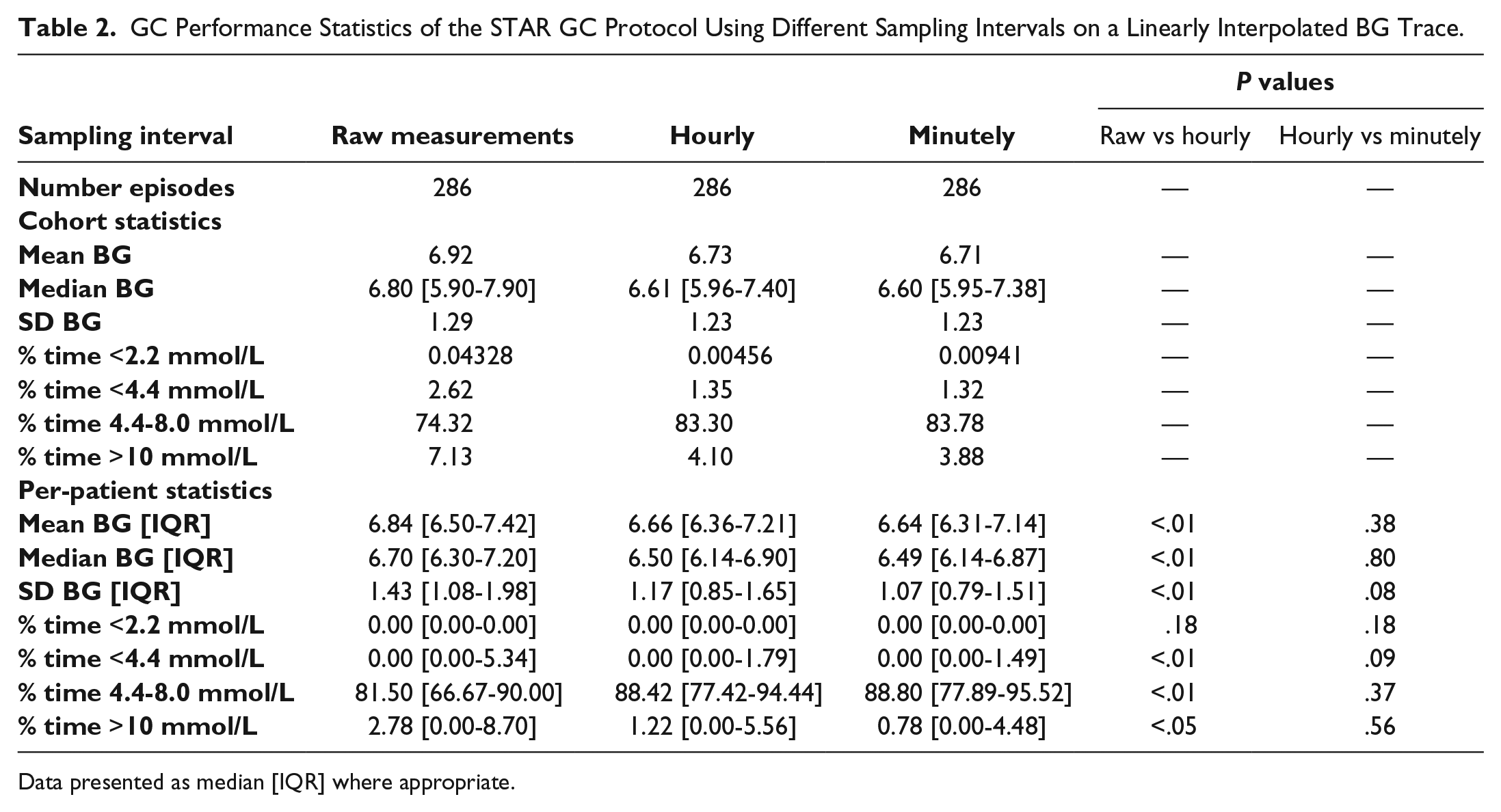
Data presented as median [IQR] where appropriate.

Figure 9 shows an example of how the various resampling techniques influence the interpretation of results. The raw measurements (x) can be seen to be dense at the beginning when the patient is out of the target band and slightly sparser within the target band. Hourly resampling (o) can be seen to more fairly capture the underlying BG trace. However, as seen at hour 29, hourly resampling can still miss key peaks in BG, dynamics that could be captured only with minutely resampling.

Figure 9.

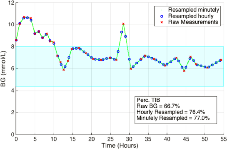
Example of the influence of resampling on time in band statistics.

Discussion

Question 1: Interpolation Techniques

Piecewise Interpolation Performance

Figure 4 shows all the piecewise interpolation techniques performed extremely well in capturing intermediate BG dynamics. Linear interpolation performed the best with an average RMSE of 0.39 mmol/L, over all the measurement intervals assessed. As the measurement interval assessed increased, so did the hidden RMSE. This result is likely due to the greater time for the intermediate BG dynamics to deviate from the interpolated trace.

Fitted Interpolation Performance

Figures 5 and 6 show a trade-off of error to the hidden and observed measurements for the fitted interpolated trace. As the KW is increased, the RMSE of the observed measurements is increased, while the RMSE of the hidden measurements is decreased. This result is due to fitted interpolation techniques becoming less erratic as the BG KW increases, as shown in Figure 8. The KW BF providing the most similar magnitude hidden and observed RMSE was chosen as the optimal, equally representing both hidden and observed measurements. The 150 minute KW 1st order B-spline BF provided the best compromise of fit to the observed (mean RMSE 1.07 mmol/L) and hidden (mean RMSE 0.80 mmol/L) measurements. Similarly, the 150 minute KW 2nd order B-spline BF also provided the best compromise of fit to the observed (mean RMSE 1.06 mmol/L) and hidden (mean RMSE 0.64 mmol/L) measurements. Note, as the variability BG levels increased the fitted interpolation techniques struggled to capture the erratic dynamics as seen in Figure 7. The restrictive nature of fitting wide knot-width BFs is shown by the increase in observed measurement error. Overall, the 2nd order B-spline BF interpolation provided the best fit to both the observed and hidden measurements of the fitted interpolation techniques investigated.

Optimal Interpolation

Although the piecewise interpolation techniques are very prone to erroneous measurements compared to the fitted interpolation techniques, which are designed to incorporate measurement error, they still provided a better estimation of the hidden measurements. The trade-off of fit between observed and hidden measurements resulted in a much larger RMSE overall for the fitted interpolation techniques compared to the piecewise interpolation techniques. In addition, the SPRINT BG values were measured using a Super-Glucocard II, which has a measurement error SD ranging from 0.15 to 0.56 mmol/L depending on the BG value.²⁵ Only the linear and cubic piecewise interpolation techniques provided a RMSE within this measurement error, providing a further independent validation that the piecewise interpolation techniques provided the best estimation of the intermediate BG dynamics.

Question 2: Sampling Analysis

Table 2 clearly shows significant differences in key GC statistics when using raw measurements compared to a sampled interpolated BG trace, for both cohort and per-patient statistics. The largest impact was seen in the median per-patient percentage of time statistics; 81.5% vs 88% BG within 4.4-8.0 mmol/L, P < .001; 2.78% vs approximately 1.0% BG > 10.0 mmol/L, P = .04. A significant difference can also be seen in the per-patient BG mean and median (mean BG of 6.84 vs 6.65 mmol/L, P = .001, and median BG of 6.7 vs 6.49 mmol/L, P = .001). This discrepancy is most likely due to the varying measurement frequency in and out of band for the STAR GC protocol, inherently causing higher numbers of raw measurements to occur outside of the targeted band than within, as seen in Figure 9. This behavior is common in GC protocols^14-19 and would result in poor measurements being overrepresented, skewing statistics.

Only a small benefit is observed from sampling the interpolated BG trace minutely compared to hourly. The largest difference occurring in the per-patient median percentage of time BG > 10 mmol/L measurements (0.78% vs 1.22%, P = .56, Table 2). This result is most likely due to the hourly sampling of the interpolated BG trace not capturing the peaks in BG seen with minutely sampling, as shown in Figure 9. This outcome is especially important when considering the number of patients within the hyper- and hypo- glycemic regions (BG > 10.0 mmol/L and BG < 4.4 mmol/L). In regard to the other statistics, a negligible difference in BG mean, and median was seen, Table 2. However, a slight difference could be seen in the per-patient SD of BG between sampling rates (1.17 vs 1.07, P = .08). Again, this result is likely due to the hourly sampling rate not capturing the full spread of the BG trace. Overall, minutely sampling had limited effect on central tendency statistics, and a greater impact on outlying events or surges, as expected.

Limitations

The SPRINT protocol has measurement intervals of 1-2 hours.¹⁴ Thus, as per protocol, the SPRINT BG data are denser in regions where a patient is variable and/or out of the targeted band. Therefore, the measurements removed (hidden measurements) to make the data sparse are more likely to be removed from the more variable and out of band BG regions (BG < 4.4 mmol/L and BG > 6.1 mmol/L). Hence, the hidden measurement error is a stronger validation test, but will likely have higher associated BG measurement error than if more stable periods were included. The results are thus a conservative estimate.

The number of observed and hidden BG measurement varies as the measurement interval assessed is increased due to the SPRINT data needing to be denser to assess smaller measurement intervals. Therefore, patients which are metabolically unstable, and thus requiring hourly BG measurements frequently, are more prone to measurement thinning compared to stable patients whom have consistently 2-hour measurement intervals. As a result, hidden measurements in this analysis may be more likely to come from unstable regions of patient data, as seen in Figure 7. However, still a significant amount data is removed from each patient per day (> 4.7/17.1 median hidden measurements per day, per patient, >27%, Table 1) providing a fair assessment of the BG interpolation techniques.

Overall, the results of this article could be applied to a variety of BG-related fields, where collected data are sparse, as it is likely that the intermediate BG dynamics will be similar between cohorts. Thus, linear interpolation and minutely or hourly resampling could also prove to be a valuable tool in diabetes modelling and assessment of GC performance. Note, the methodology presented in this article could also be used to assess the current methods used for GC performance assessment and modelling, provided a dense enough data set was available.

Conclusion

This study investigated two main questions in analyzing BG data. First, BG measurement interpolation techniques to represent intermediate BG dynamics and the observed measured BG. Second, the effect of resampling rate on the interpolated BG trace GC performance metrics. Answering these two questions will enable fair, accurate GC performance assessment and comparison, avoiding significant potential bias.

Overall, the linear piecewise interpolation performed the best of all interpolation techniques investigated (mean RMSE 0.39 mmol/L), providing the best estimate of the intermediate, hidden BG dynamics. The fitted interpolation techniques failed to capture the hidden BG measurements without providing a poor fit to the observed measurements. Thus, linear piecewise interpolation provides the best estimate of intermediate BG dynamics and should be used.

The effect of resampling interpolated retrospective BG data on key GC performance metrics found a significant difference when comparing raw to resampled interpolated BG measurements. The difference is especially important when the GC protocols being investigated have varying measurement intervals depending on the BG value. Therefore, for fair, unbiased comparison of a GC protocol’s performance, minutely resampled linear piecewise interpolation of BG results is the best option.

The techniques presented in this article provide a general solution to approximate the intermediate BG dynamics of commonly seen in sparse ICU BG data and may prove useful in other clinical areas, including diabetes.

Footnotes

Abbreviations

BF, basis function; BG, blood glucose; GC, glycaemic control; ICU, intensive care unit; IQR, interquartile range; KW, knot width; RMSE, root mean square error; SD, standard deviation; SPRINT, Specialized Relative Insulin-Nutrition Tables; STAR, Stochastic TARgeted.

Authors’ Note

The Upper South Regional Ethics Committee, New Zealand granted approval for the audit, analysis, and publication of these data. The datasets used and/or analyzed during the current study are available from the corresponding author on reasonable request.

Declaration of Conflicting Interests

The author(s) declared no potential conflicts of interest with respect to the research, authorship, and/or publication of this article.

Funding

The author(s) disclosed receipt of the following financial support for the research, authorship, and/or publication of this article: We acknowledge the support of UC Doctoral Scholarships for Kent Stewart, as well as funding from EU FP7, RSNZ IRSES mobility grants, the HRC of NZ, and the NSC 2010.

ORCID iD

Kent W. Stewart

References

Gartemann

Caffrey

Hadker

Crean

Creed

Rausch

. Nurse workload in implementing a tight glycaemic control protocol in a UK hospital: a pilot time-in-motion study. Nurse Crit Care. 2012;17(6):279-284.

Carayon

Gürses

. A human factors engineering conceptual framework of nursing workload and patient safety in intensive care units. Intensive Crit Care Nurs. 2005;21(5):284-301.

Bellazzi

Nucci

Cobelli

. The subcutaneous route to insulin dependent diabetes therapy. IEEE Eng Med Biol Mag. 2001;20(1):54-64.

Malesker

Foral

McPhillips

Christensen

Chang

Hilleman

. An efficiency evaluation of protocols for tight glycemic control in intensive care units. Am J Crit Care. 2007;16(6):589-598.

Evans

Le Compte

Tan

et al . Stochastic targeted (STAR) glycemic control: design, safety, and performance. J Diabetes Sci Technol. 2012; 6(1):102-115.

Bergman

Phillips

Cobelli

. Physiologic evaluation of factors controlling glucose tolerance in man: measurement of insulin sensitivity and beta-cell glucose sensitivity from the response to intravenous glucose. J Clin Invest. 1981;68(6):1456-1467.

Mari

Valerio

. A circulatory model for the estimation of insulin sensitivity. Control Eng Pract. 1997;5(12):1747-1752.

Parker

Doyle

III . Control-relevant modeling in drug delivery. Adv Drug Deliv Rev. 2001;48(2-3):211-228.

Lotz

Chase

McAuley

et al . Integral-based identification of a physiological insulin and glucose model on euglycaemic clamp and IVGTT trials. IFAC Proc Vol. 2006;39(1):463-468.

10.

Wong

Chase

Shaw

et al . Model predictive glycaemic regulation in critical illness using insulin and nutrition input: a pilot study. Med Eng Phys. 2006;28(7):665-681.

11.

Chase

Wong

Singh-Levett

et al . Simulation and initial proof-of-concept validation of a glycaemic regulation algorithm in critical care. Control Eng Pract. 2008;16(3):271-285.

12.

Hovorka

Chassin

Ellmerer

Plank

Wilinska

. A simulation model of glucose regulation in the critically ill. Physiol Meas. 2008;29(8):959.

13.

Lin

Razak

Pretty

et al . A physiological Intensive Control Insulin-Nutrition-Glucose (ICING) model validated in critically ill patients. Comput Methods Programs Biomed. 2011;102(2):192-205.

14.

Chase

Shaw

Le Compte

et al . Implementation and evaluation of the SPRINT protocol for tight glycaemic control in critically ill patients: a clinical practice change. Crit Care. 2008;12(2):R49.

15.

NICE-SUGAR Study Investigators. Intensive versus conventional glucose control in critically ill patients. N Engl J Med. 2009;360(13):1283-1297.

16.

Preiser

Devos

Ruiz-Santana

et al . A prospective randomised multi-centre controlled trial on tight glucose control by intensive insulin therapy in adult intensive care units: the Glucontrol study. Intensive Care Med. 2009;35(10):1738.

17.

Amrein

Ellmerer

Hovorka

et al . Efficacy and safety of glucose control with Space Glucose Control in the medical intensive care unit—an open clinical investigation. Diabetes Technol Ther. 2012;14(8):690-695.

18.

Van Herpe

Mesotten

Wouters

et al . LOGIC-insulin algorithm–guided versus nurse-directed blood glucose control during critical illness: the LOGIC-1 single-center, randomized, controlled clinical trial. Diabetes Care. 2013;36(2):188-194.

19.

Stewart

Pretty

Tomlinson

et al . Safety, efficacy and clinical generalization of the STAR protocol: a retrospective analysis. Ann Intensive Care. 2016;6(1):24.

20.

Pretty

Le Compte

Shaw

Chase

. Impact of sensor and measurement timing errors on model-based insulin sensitivity. IFAC Proc Vol. 2012;45(18):224-229.

21.

Chase

Andreassen

Jensen

Shaw

. Impact of human factors on clinical protocol performance: a proposed assessment framework and case examples. J Diabetes Sci Technol. 2008;2:409-416.

22.

Finfer

Wernerman

Preiser

et al . Clinical review: consensus recommendations on measurement of blood glucose and reporting glycemic control in critically ill adults. Crit Care. 2013;17(3):229.

23.

Evans

Le Compte

Tan

et al . Stochastic targeted (STAR) glycemic control: design, safety, and performance. J Diabetes Sci Technol. 2012;6(1):102-115.

24.

De Boor

. On calculating with B-splines. J Approx Theory. 1972;6:50-62.

25.

Arkray. Glucocard™ Test Strip 2 Data Sheet. Japan: Arkray Inc; 2007.

26.

Bonferroni

. Teoria statistica delle classi e calcolo delle probabilita. Florence, Italy: Libreria internazionale Seeber; 1936.

Interpretation of Retrospective BG Measurements

Abstract

Background:

Methods:

Results:

Conclusion:

Keywords

Methods

Patient Data

Question 1: Interpolation Techniques

Piecewise Interpolation

Fitted Interpolation

Interpolation Analysis

Question 2: Sampling Analysis

Results

Question 1: Piecewise Interpolation

Question 1: Fitted Interpolation

Question 2: Sampling Interval

Discussion

Question 1: Interpolation Techniques

Piecewise Interpolation Performance

Fitted Interpolation Performance

Optimal Interpolation

Question 2: Sampling Analysis

Limitations

Conclusion

Footnotes

Abbreviations

Authors’ Note

Declaration of Conflicting Interests

Funding

ORCID iD

References