
Abstract
Background:
Linear empirical dynamic models have been widely used for glucose prediction. The extension of the concept of seasonality, characteristic of other domains, is explored here for the improvement of prediction accuracy.
Methods:
Twenty time series of 8-hour postprandial periods (PP) for a same 60g-carbohydrate meal were collected from a closed-loop controller validation study. A single concatenated time series was produced representing a collection of data from similar scenarios, resulting in seasonality. Variability in the resulting time series was representative of worst-case intrasubject variability. Following a leave-one-out cross-validation, seasonal and nonseasonal autoregressive integrated moving average models (SARIMA and ARIMA) were built to analyze the effect of seasonality in the model prediction accuracy. Further improvement achieved from the inclusion of insulin infusion rate as exogenous variable was also analyzed. Prediction horizons (PHs) from 30 to 300 min were considered.
Results:
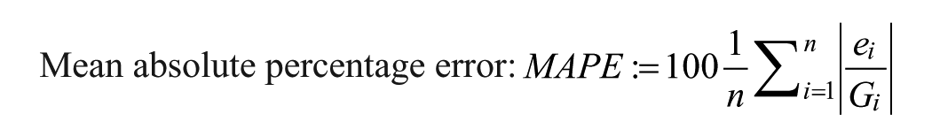
SARIMA outperformed ARIMA revealing a significant role of seasonality. For a 5-h PH, average MAPE was reduced in 26.62%. Considering individual runs, the improvement ranged from 6.3% to 54.52%. In the best-performing case this reduction amounted to 29.45%. The benefit of seasonality was consistent among different PHs, although lower PHs benefited more, with MAPE reduction over 50% for PHs of 60 and 120 minutes, and over 40% for 180 min. Consideration of insulin infusion rate into the seasonal model further improved performance, with a 61.89% reduction in MAPE for 30-min PH and reductions over 20% for PHs over 180 min.
Conclusions:
Seasonality improved model accuracy allowing for the extension of the PH significantly.
An important feature of any artificial pancreas1,2 is its ability to predict glucose along a given prediction horizon (PH), either as part of the control algorithm itself, such as in systems based on model predictive control (MPC) techniques,3-5 or as part of a monitoring subsystem to predict, for instance, hypoglycemic episodes.6-8 Model requirements and input information will depend on the specific purpose. For instance, future values of insulin infusion are available during the MPC optimization process where predictions are needed. However, this is not the case in the context of risk prediction in patient monitoring during closed-loop operation.
Linear empirical dynamic models rely on time series as an observation on a dynamic system. 9 These include autoregressive (AR), autoregressive moving average (ARMA), and autoregressive models with exogenous inputs (ARX), among others. These models have been widely used in the context of glucose prediction. Gani et al 10 identified 30th-order AR models from continuous glucose monitoring (CGM) data with 1-min sampling time from nine T1D subjects. An average root mean square error (RMSE) of 12.6 mg/dL was reported for a 60-min PH, after data smoothing and parameter regularization. Sparacino and colleagues 11 identified a 1st-order time-varying AR model based on data from 28 T1D subjects wearing a microdialysis system with a 3-min sampling time. They demonstrated the feasibility of predicting hypoglycemic events 20-25 min ahead in time, considering a 30-min PH. A median RMSE ranging from 18.33 to 20.32 mg/dL, depending on the selection of a forgetting factor, was reported for that PH. Low-order AR and ARMA models were considered by Eren-Oruklu and associates 12 considering PHs up to 30 minutes in healthy and type 2 diabetes subjects. A sum of squares of glucose prediction error ranging between 10.32 and 12.55 mg/dL was reported, depending on the study, for a 30-min PH. Finan and colleagues13-15 evaluated ARX models from simulated and clinical ambulatory data with 5-min sampling time. The authors concluded that 60 minutes was a maximum achievable PH in terms of model prediction accuracy. An average RMSE of 26, 34 and 40 mg/dL was reported for 30-, 45-, and 60-min PH, respectively. 15 This corresponds to an improvement of 9% compared to a zero-order-hold predictor. A variety of linear and nonlinear time-series models were evaluated by Ståhl and Johansson 16 from clinical data from one subject, with nonuniform and sparse sampling (fingerstick measurements) with spline interpolation, in order to produce a short-term blood glucose predictors for up to two-hour-ahead blood glucose prediction. However, many difficulties were met not achieving the required accuracy.
Empirical dynamic models are also widely used in other domains such as business and economic time series. A particular characteristic in these domains is seasonality, that is, the existence of regular patterns of changes and fluctuations that repeat periodically. 17 This article explores the extension of the concept of seasonality for glucose prediction with a proof-of-concept study. The main rationale is that preprocessing of CGM time series (and available additional information) may translate daily events into seasonal phenomena. For instance, glucose concentration tends to peak and then decline in a characteristic way after a meal intake in a particular scenario. In this case, a new preprocessed family of time series can be built from the original CGM data by concatenating postprandial periods (PPs) of fixed length where similarity of behaviors is expected, according to some metrics, which would theoretically produce seasonal time series. This allows for the application of seasonal models that exploit this similarity for more accurate predictions and longer PHs. Seasonal autoregressive integrated moving average (SARIMA) models are considered in this work and compared to its nonseasonal counterpart in order to investigate the benefit of seasonality into glucose prediction. The use of insulin infusion rate as an exogenous variable is also explored.
Methods
Data Overview
CGM time series covering 8-hour PPs for a same meal were collected from the Clinic University Hospital of Valencia, Spain. Data belonged to a closed-loop controller validation study where 10 T1D subjects underwent an in-hospital 8-hour standardized mixed meal test (60g carbohydrate) on two occasions with a hybrid artificial pancreas with 15-min sampling period. Patients wore two pumps with CGM devices (Paradigm Veo® insulin pump with Enlite-2 sensors®, Medtronic MiniMed, Northridge, CA, USA), which were calibrated 15 minutes before the meal test was administered (lunch at noon). CGM glucose data were available for eight hours after the meal, from 12:00
Despite meal size was controlled in this in-patient study, this didn’t prevent the presence of high intra- and interindividual variability. These were measured by the coefficient of variance of the area under the curve for the 8-hour duration of the study (CV-AUC8h), which was computed with the trapezoidal rule. Euclidean distance among paired PPs was also computed to determine time series shape similarity. A sampling period of 15 minutes was considered to match glucose reference measurements and our controller configuration.
SARIMA Model
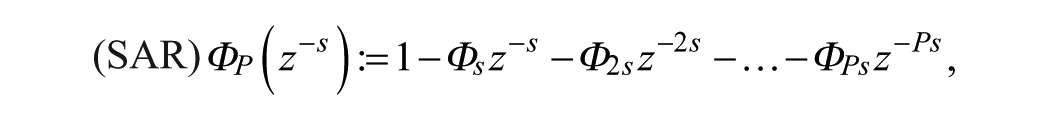
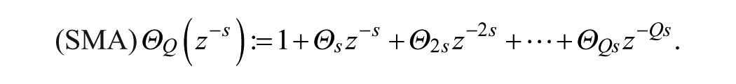
A SARIMA model is an expanded form of its nonseasonal counterpart ARIMA model that includes as new model components seasonal autoregressive (SAR) and seasonal moving-average (SMA) terms. In an empirical dynamic model, an observation at time
Given a CGM time series

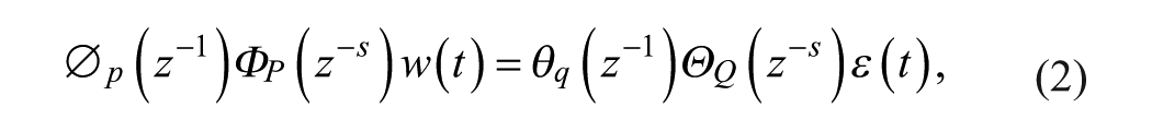
where


Model (1)-(2) can be expressed in short form as SARIMA
Exogenous Variables
Exogenous variables in model (1)-(2) were also considered. There exist different approaches for incorporating exogenous variables into a model. Denoting as


when current and past values of the exogenous variable
Identification Procedure
Box-Jenkins methodology9,19 was used for model building and evaluation (see Figure 1). A leave-one-out cross-validation procedure was considered dividing data into training and validation sets. In order to avoid data from a same patient to appear both in training and validation, data from the validation patient was excluded from the training set. This resulted in 18 PPs for training and 1 for validation, since two CL studies per patient were available. PPs in the training set were randomly ordered at each run according to a random sequence generator (www.random.org). A stationarity analysis was first carried out with the unit-root test (Augmented Dickey-Fuller test).
20
The backward-difference operator ∇ was applied to the time series as many times as necessary (integration order


where
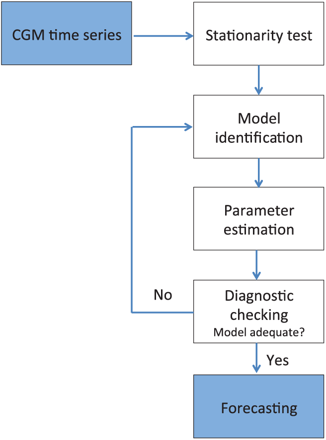
Steps for building a good model through Box-Jenkins methodology.
Results
Figure 2 shows the dataset resulting from the concatenation of the twenty 8-h PPs. The CGM time series had a mean of 136.1 mg/dL, with a standard deviation of 48.48 mg/dL. Despite the same meal was provided, data exhibited high variability with postprandial peaks ranging from 304 mg/dL (P91) to 125 mg/dL (P42) and the incidence of hypoglycemia in some patients (P11, P51, P52, P71, P101), two of them severe (P11, P101), according to CGM values. They were nonnormally distributed. Interindividual variability measured by CV-AUC8h was 21.52%, whereas intraindividual variability was 9.17%. However, the latter spanned from 3.22% (patient 6) to 18.67% (patient 9). Since only two studies per patient were available, intrapatient variability might be underestimated. It is thus considered that worst-case intrapatient variability is represented by the generated time series. Euclidean distance between each pair of PPs was also computed to analyze similarity of time series (see Figure 3), providing similar conclusions. Patient 9 is the most dissimilar among studies (green box in P91-P92), only exceeded by comparatively few yellow-red boxes outside the diagonal (between-patient comparisons). P81, P82, and P91 were the most dissimilar with the rest of periods (higher incidence of yellow-red boxes). Total basal insulin infusion in the 8-h period ranged from 5.21U (P31) to 16.40U (P71). An extended bolus computed from the patient’s insulin-to-carbohydrate ratio and open-loop basal infusion rate was also administered at meal time.
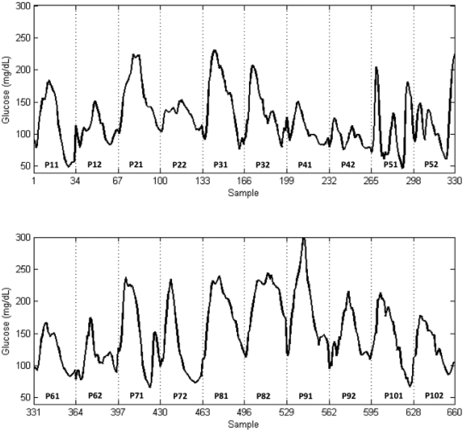
CGM time series resulting from the concatenation of twenty 8-h PPs for a same 60g carbohydrate meal. The notation Pij is used to name the different periods, where i is the number of the patient,
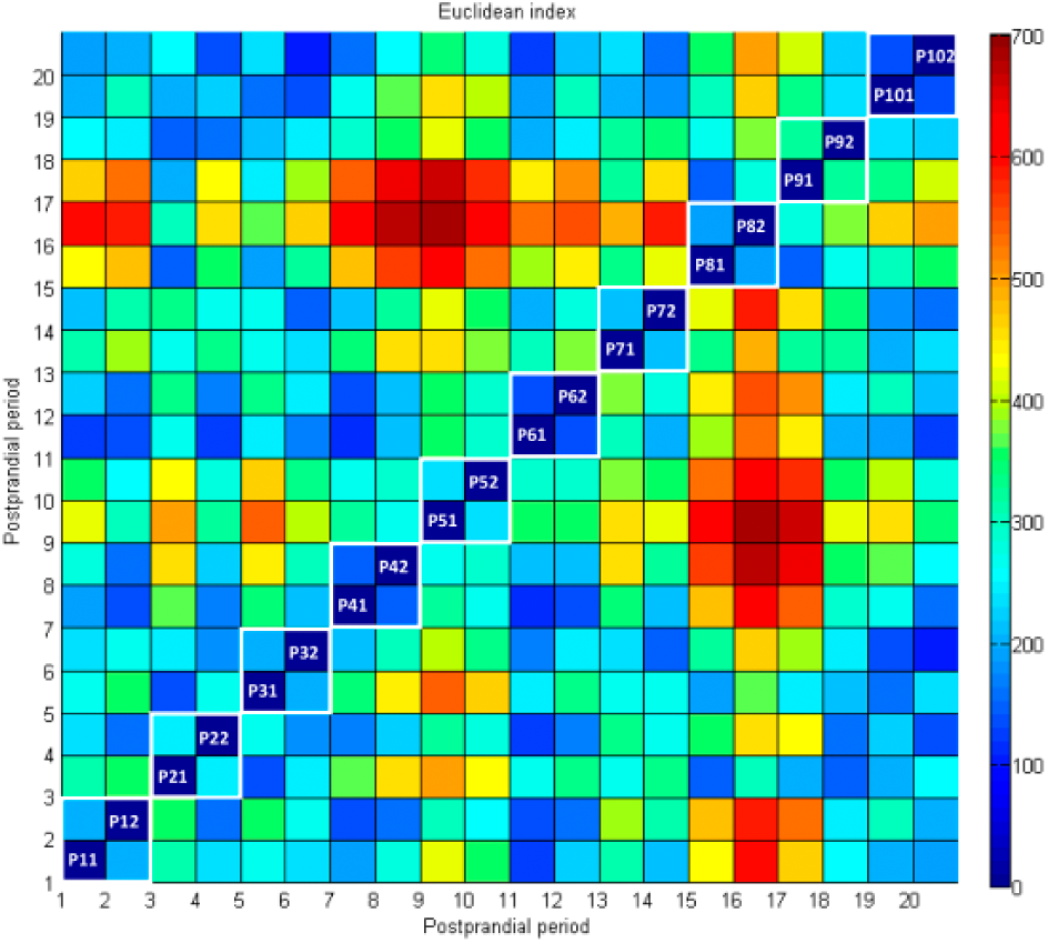
Similarity among PPs in the CGM time series as measured by the Euclidean distance between paired periods. Data is shown according to the color scale in the right. White boxes in the diagonal indicate periods corresponding to a same patient.
Both SARIMA and ARIMA models were identified for each run in the cross-validation. Figure 4(a) shows the forecasting accuracy metrics for a 5-h PH for both cases. A high PH was initially chosen to challenge the model. SARIMA outperform ARIMA in all metrics (mean(SD): MAE(mg/dL) 34.56(19.35) vs 47.72(24.43); RMSE(mg/dL) 40.02(21.62) vs 55.02(26.93); MAPE(%) 22.02(9.41) vs 30.01(13.05); P < .05 in all cases). In the following, the analysis will be restricted to MAPE since the three measures provided the same information. Figure 4(b) shows the obtained MAPE as the PH increases from 30 min to 5 hours, consistently outperforming SARIMA. The identified model structure differed slightly between runs, with AR and MA orders up to 4. No time series differentiation was needed for both ARIMA and SARIMA models. Seasonality with lag 33 (the size of the PP) was obtained in all cases, as expected. SAR and SMA orders were up to 2.
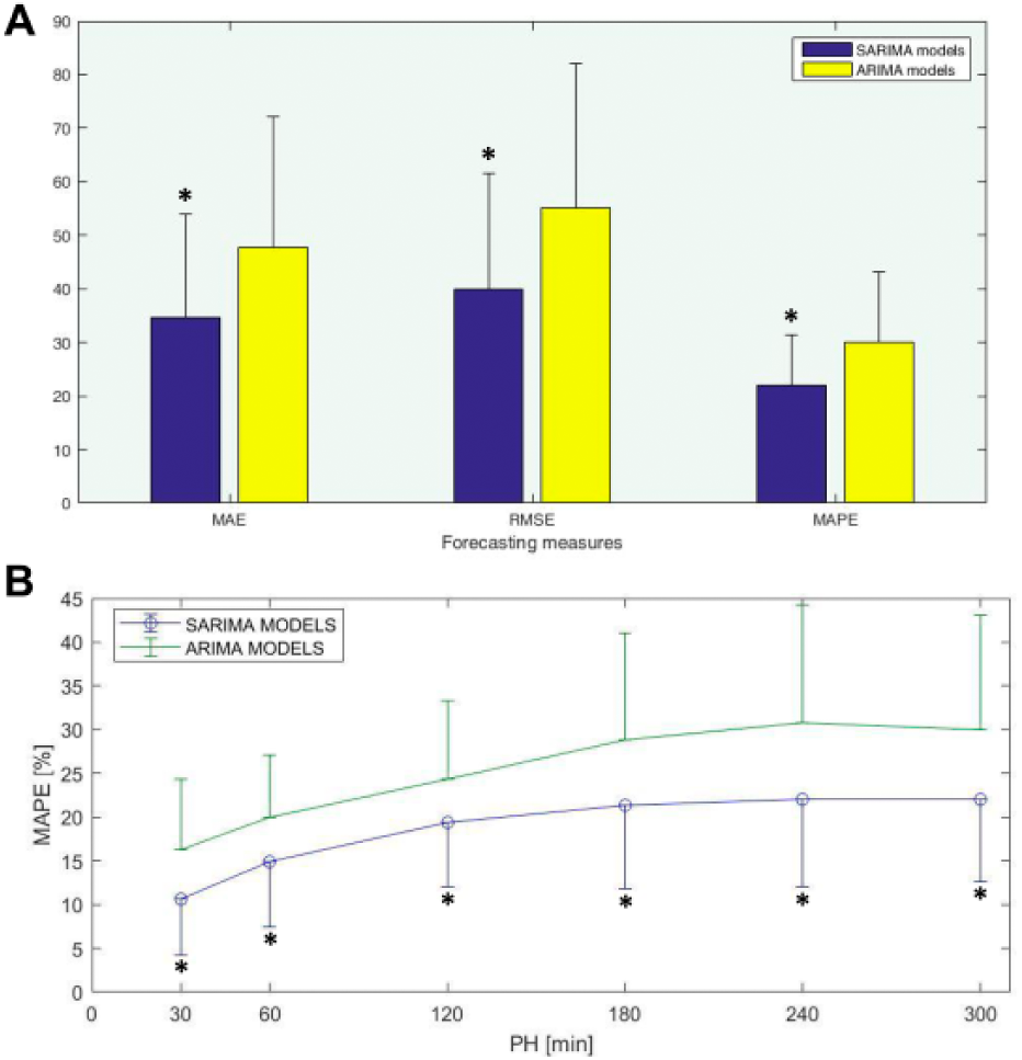
Forecasting performance: (a) Mean and standard deviation of forecasting measures for the 20-fold cross-validation and a 5-h PH: MAE(mg/dL) is Mean Absolute Error; RMSE(md/dL) is Root Mean Square Error; MAPE(%) is Mean Absolute Percentage Error; (b) Mean and standard deviation of MAPE(%) for increasing values of the prediction horizon. *P < .05.
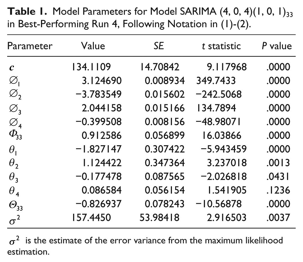
The best performing run was Run 4, with validation data P22. In this case, inspection of the ACF revealed data were stationary (the trend had a nonsignificant P value of .0877) and seasonal at lag 33 with a significant P value of .0000. Seasonally differenced data were stationary with significant P value of .0001, so it was not necessary to take any difference. Model SARIMA
Model Parameters for Model SARIMA (4, 0, 4)(1, 0, 1)33 in Best-Performing Run 4, Following Notation in (1)-(2).
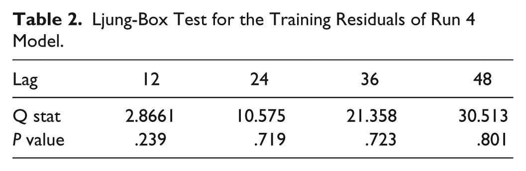
Ljung-Box Test for the Training Residuals of Run 4 Model.
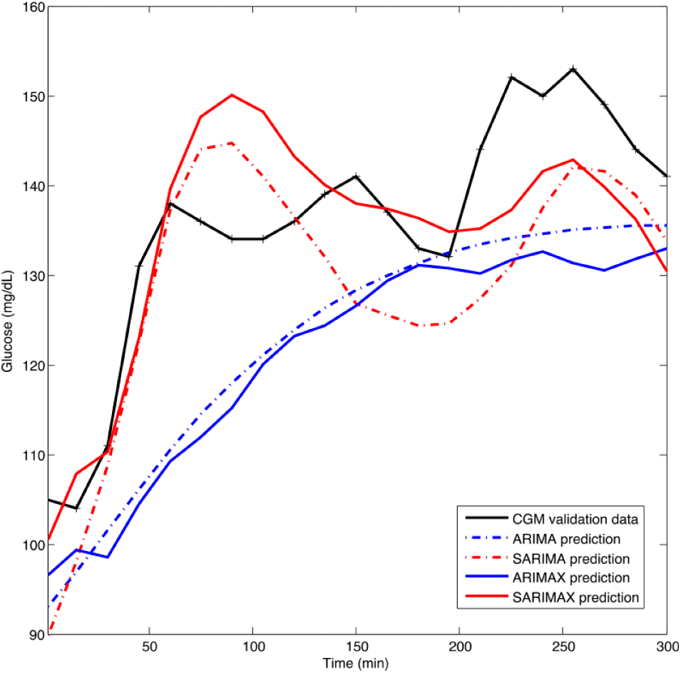
Forecasting of models ARIMA(4, 0, 4), SARIMA(4, 0, 4)(1, 0, 1)33, ARIMAX(4, 0, 4, 2) and SARIMAX(4, 0, 4, 2)(1, 0, 1)33 for Run 4 considering a 5-h prediction horizon.
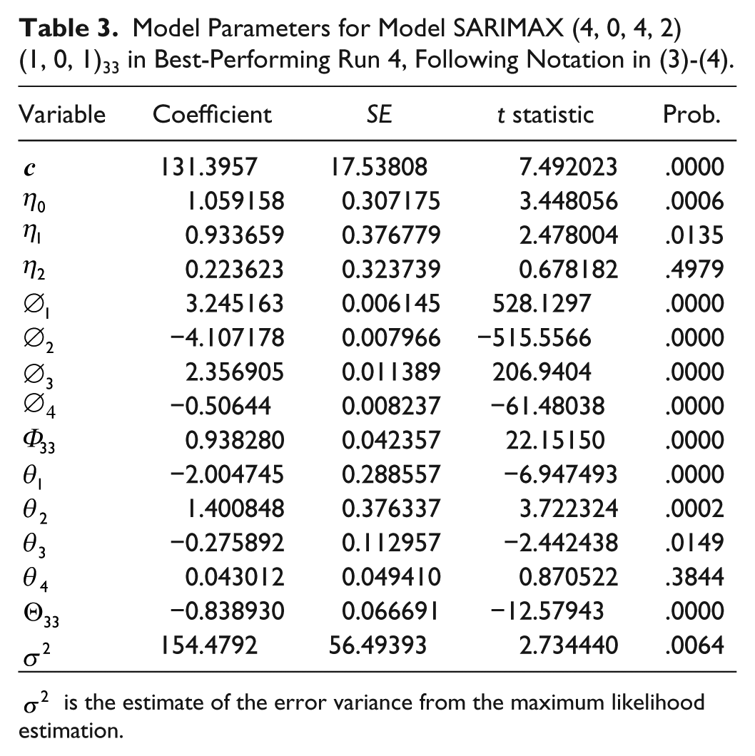
The effect of considering insulin infusion as exogenous variable for performance improvement was investigated. Besides, insulin infusion information is needed in applications such as MPC. This analysis was carried out only for Run 4 as the best performing case, challenging further improvement. Insulin infusion signal contained bolus and basal infusion and was expressed in U per sampling period. Granger causality test was applied to test the null hypothesis that CGM does not “Granger cause” insulin infusion and vice versa. The null hypothesis was rejected with a significant P value of .0146. Therefore, inclusion of insulin infusion into the model might improve performance. The order of the exogenous polynomial was computed from the cross-correlation plot and AIC, resulting in the model SARIMAX
Model Parameters for Model SARIMAX (4, 0, 4, 2)(1, 0, 1)33 in Best-Performing Run 4, Following Notation in (3)-(4).
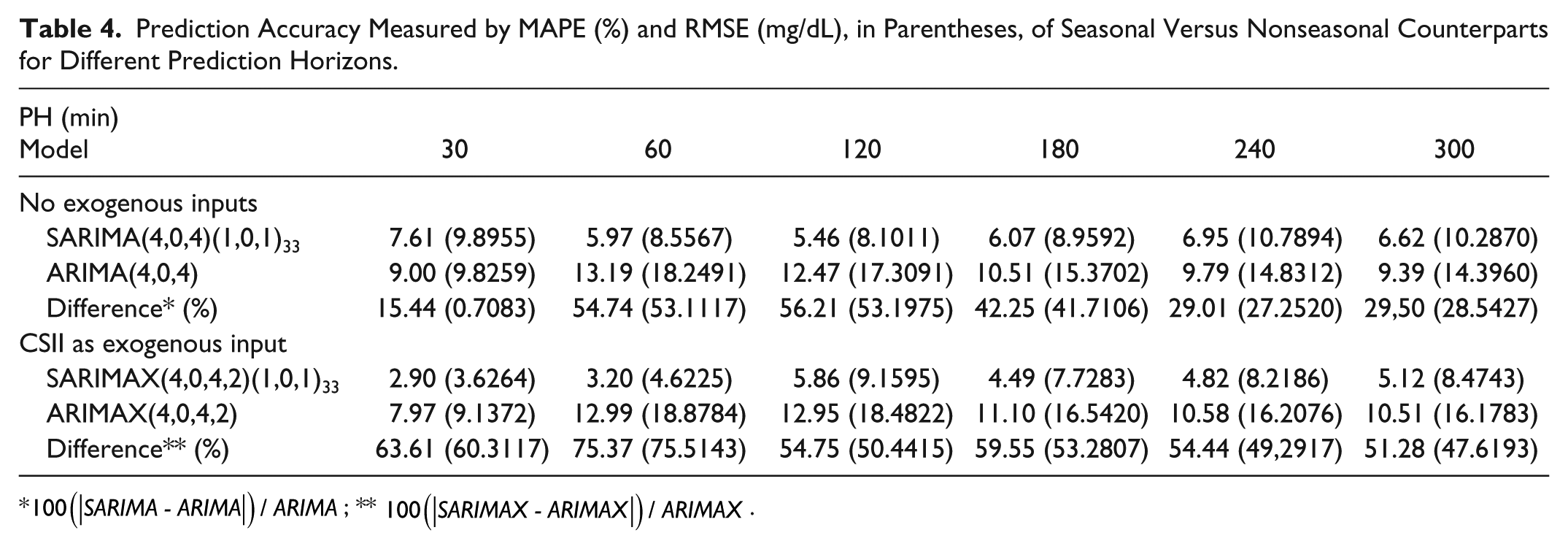
Finally, forecasting performance as measured by MAPE and RMSE at different PHs is presented in Table 4. PHs of 30, 60, 120, 180, 240, and 300 minutes were considered.
Prediction Accuracy Measured by MAPE (%) and RMSE (mg/dL), in Parentheses, of Seasonal Versus Nonseasonal Counterparts for Different Prediction Horizons.
Discussion
Training data consisted in a collection of PPs from different patients covering both early and late postprandial phases (8 hours). Time between meals during the day is generally shorter. Nocturnal period was not represented by our data. However, PP has shown to be much more challenging than nocturnal period for an artificial pancreas. 23 Both CV-AUC8h and Euclidean distance (Figure 3) showed large interindividual variability and a large range in intraindividual variability, with its worst-case represented by interindividual variability. Thus, the concatenated time series defines a challenging scenario with a worst-case highly variable patient. Data variability might be attenuated with the use of classification techniques, collecting similar enough postprandial responses into different datasets, with their corresponding prediction model.
A first-order seasonal AR and MA component was identified with seasonality lag 33 in all SARIMA runs due to the concatenated nature of the time series. In all runs, SARIMA outperformed ARIMA revealing a significant role of seasonality. 5-h PH average MAPE was reduced in 26.62%. Considering individual runs, the improvement ranged from 6.3% (Run 7; validation data P41) to 54.52% (Run 3; validation data P21). In the best performing case, according to MAPE (Run 4), this reduction amounted to 29.45%. Prediction improvement by introducing seasonality also becomes apparent from Figure 5. The benefit of seasonality was consistent among different PHs, as illustrated in Figure 4(b) and Table 4 for Run 4. Lower PHs benefited more, with a MAPE reduction over 50% for PHs of 60 and 120 minutes, and over 40% for 180 min. In these case, MAPE was close to 6% and RMSE below 10 mg/dL, doubling these values when seasonality was not considered. In greater PHs benefit of seasonality is still observed, although decreasing due to variability in the time series.
Consideration of insulin infusion rate into the seasonal model further improved performance for Run 4. Although analysis was limited to this case to reduce computational burden, remark it corresponds to the most challenging situation for model improvement since SARIMA model for Run 4 has the best prediction accuracy in the cross-validation study. SARIMAX improved performance as compared to SARIMA with a 61.89% reduction in MAPE (2.90% vs 7.61%) for 30-min PH to a 7.33% reduction at 2-h PH (5.86% vs 5.46%) and reductions over 20% for PHs over 180 min, as shown in Table 4. A RMSE below 10 mg/dL was obtained for all PHs. This means that SARIMAX models might allow the increment of PHs in MPC-based artificial pancreas systems. Table 4 also shows that SARIMAX outperformed in all cases its nonseasonal counterpart ARIMAX.
This is a proof-of-concept study and as such it has limitations. It is assumed that mealtime is known, allowing for the construction of concatenated time series with fixed-length PPs. However, to date, meal announcement is a common component of artificial pancreas systems and, otherwise, meal detection algorithms are incorporated.24-26 Remark that although focus was put on PPs, this approach can be applied to other fixed-length time series data subsets representing characteristic scenarios where similarity is expected or learned from classification techniques. Another limitation is the data used, which did not correspond to a single patient, although interpatient variability in the data was representative of worst-case intrapatient variability defining a challenging scenario. A collection of 18 PPs were used for model training at each cross-validation run. Seasonal components of the identified models were first or second order, which means that current meal depends, at most, on the two previous similar meals. Thus, the length of the data used is considered appropriate for this proof-of-concept study. However, further investigation is needed with longer single-patient CGM data and the combination of seasonal modelling with classifiers.
Conclusion
Despite the limitations of this study, seasonality has shown to be an important factor to improve model predictive power allowing for the significant extension of PHs. Further work is now needed for the classification of periods under scenarios yielding “similar enough” glycemic responses to fully exploit the expected benefit of seasonal models.
Footnotes
Acknowledgements
The authors acknowledge the collaboration of Paolo Rossetti from Hospital Francesc de Borja de Gandia, F.J. Ampudia-Blasco from Hospital Clínico Universitario de Valencia, I. Conget, M. Giménez, and C. Quirós from Hospital Clinic de Barcelona, and J. Vehí from Universitat de Girona who participated in the implementation and/or design of the study from which data were obtained, as well as the altruist participation of all the patients involved in the study.
Abbreviations
ACF, autocorrelation function; AIC, Akaike information criterion; AP, artificial pancreas; AR, autoregressive; ARIMA, autoregressive integrated moving average; ARIMAX, autoregressive integrated moving average with exogenous variables; ARMA, autoregressive moving average; ARX, autoregressive with exogenous inputs; CGM, continuous glucose monitoring; CSII, continuous subcutaneous insulin infusion; MAE, mean absolute error; MAPE, mean absolute percentage error; MPC, model predictive control; PACF, partial autocorrelation function; PH, prediction horizon; PP, postprandial period; RMSE, root mean square error; SAR, seasonal autoregressive; SARIMA, seasonal autoregressive integrated moving average; SARIMAX, seasonal autoregressive integrated moving average with exogenous variables; SMA, seasonal moving average; T1D, type 1 diabetes.
Declaration of Conflicting Interests
The author(s) declared no potential conflicts of interest with respect to the research, authorship, and/or publication of this article.
Funding
The author(s) disclosed receipt of the following financial support for the research, authorship, and/or publication of this article: This work was funded by the Spanish Ministry of Economy and Competitiveness, grants DPI2013-46982-C2-1-R and DPI2016-78831-C2-1-R, and the European Union through FEDER funds.