Sage Journals: Discover world-class research

Abstract

Background:

A reliable model of the probability density function (PDF) of self-monitoring of blood glucose (SMBG) measurement error would be important for several applications in diabetes, like testing in silico insulin therapies. In the literature, the PDF of SMBG error is usually described by a Gaussian function, whose symmetry and simplicity are unable to properly describe the variability of experimental data. Here, we propose a new methodology to derive more realistic models of SMBG error PDF.

Methods:

The blood glucose range is divided into zones where error (absolute or relative) presents a constant standard deviation (SD). In each zone, a suitable PDF model is fitted by maximum-likelihood to experimental data. Model validation is performed by goodness-of-fit tests. The method is tested on two databases collected by the One Touch Ultra 2 (OTU2; Lifescan Inc, Milpitas, CA) and the Bayer Contour Next USB (BCN; Bayer HealthCare LLC, Diabetes Care, Whippany, NJ). In both cases, skew-normal and exponential models are used to describe the distribution of errors and outliers, respectively.

Results:

Two zones were identified: zone 1 with constant SD absolute error; zone 2 with constant SD relative error. Goodness-of-fit tests confirmed that identified PDF models are valid and superior to Gaussian models used so far in the literature.

Conclusions:

The proposed methodology allows to derive realistic models of SMBG error PDF. These models can be used in several investigations of present interest in the scientific community, for example, to perform in silico clinical trials to compare SMBG-based with nonadjunctive CGM-based insulin treatments.

Keywords

measurement error modeling parameter estimation self-monitoring blood glucose statistical distribution

In the conventional type 1 diabetes (T1D) therapy, blood glucose (BG) concentration is maintained within its normal range by exogenous insulin administrations that are tuned by the patient himself/herself based on self-monitoring of blood glucose (SMBG) measurements, collected in a small drop of capillary blood by portable BG meters.¹ SMBG measurements are affected by measurement error which can negatively impact the effectiveness of the patient’s therapeutic decisions. For example, an underestimation of BG concentration can lead to a too small insulin dose which may result in hyperglycemia, that, when prolonged and frequently repeated in time, can lead to long-term complications like cardiovascular diseases, neuropathy, nephropathy and retinopathy; conversely, an overestimation of BG concentration can lead to a too large insulin dose which exposes the patient at risk of hypoglycemia, that can drive, in the short-term, to risky conditions like seizure and coma and even to death.

In the past 20 years, glucose monitoring has been revolutionized by the introduction of continuous glucose monitoring (CGM) devices,² minimally invasive sensors that measure glucose concentration in the subcutis every 1-5 min for up to 7-14 days. The use of CGM sensors can be very beneficial for the glycemic control and quality of life of T1D patients, but currently most CGM sensors are approved to be used only as adjunctive devices to support, but not to substitute, the use of SMBG for making treatment decisions (the only CGM devices currently approved for nonadjunctive use are the Dexcom G5 Mobile and, in Europe, the Abbott Freestyle Libre). Determining if CGM is safe and effective enough to substitute SMBG in diabetes management has therefore become a hot topic of investigation for the diabetes research community and regulatory agencies. Computer simulations can be very helpful in this because they allow to perform the so-called in silico clinical trials (see also the outcome of a recent FDA panel meeting).^3,4 Of course, to perform an in silico clinical trial comparing CGM-based to SMBG-based treatment, realizations of SMBG and CGM measurement error must be generated in silico, as well as the patient’s physiological response to these treatments. While robust models of CGM error and T1D patient physiology can be found in the literature,^5,6 a reliable model of the SMBG measurement error is still missing.

Of course, the simplest strategy that could be used to generate in silico realizations of SMBG measurement error is the bootstrap approach of sampling from a data set of SMBG error realizations derived from data. However, a limitation of this approach is that the number of different SMBG error realizations that can be simulated is finite (and, in particular, equal to the cardinality of the data set available). This is a problem for large-scale in silico applications, such as an in silico clinical trial with long study duration and/or a large number of virtual subjects involved. This limitation is of course overtaken by the availability of a mathematical model of SMBG error, which allows generating an unlimited number of SMBG error realizations.

In the literature, a very simple model of SMBG measurement error was proposed which assumes (1) uncorrelation between consecutive SMBG values (at variance with CGM, whose quasi-continuous nature allowed descriptions of the measurement error autocorrelation by using 1st or 2nd order autoregressive models)^5,7-10 and (2) the error to be proportional to the glucose concentration (ie, relative) all over the entire glucose range and described by a Gaussian function.^11-13 However, to the best of our knowledge, this simple model has never been validated and several evidences in the literature suggest that it is suboptimal. In particular, while the assumption of uncorrelation between samples is reasonable because of the sparseness of SMBG measurements (usually collected 4-5 times per day), a critical point concerns the use of a single canonical probability density function (PDF) valid over the entire BG range. As a matter of fact, the scatterplots reported in Freckmann et al^14-16 show that neither absolute nor relative error of SMBG data presents constant mean and standard deviation (SD) over the entire BG range, suggesting that a multizone model, that is, a function with different parameters in different BG ranges, is properly needed to describe SMBG error distribution. Attempts to deal with this issue include the work by Breton and Kovatchev,¹⁷ where a Gaussian model with zero mean and SD dependent on the BG value was adopted, and that by Karon et al,¹⁸ where SMBG measurements were simulated by two different strategies (the first exploiting the Gaussian distribution model with different values of mean and SD, the second based on a Gaussian distribution model whose mean is sampled from a pool of high-accuracy reference measurements) which were subsequently empirically validated.¹⁹ In Pretty et al²⁰ a bivariate kernel density model of SMBG measurements given reference values was derived for the Abbott Optium Xceed (Abbott Diabetes Care, Alameda, CA) device. Another critical point concerns the symmetry assumption of SMBG measurement error distribution made with the Gaussian model of the PDF. The histograms reported in Chan et al²¹ show that some SMBG devices present an asymmetric error distribution, calling for the use of models of the PDF allowing for nonzero skewness.

The aim of this contribution is to develop a new method to derive a model of the PDF of SMBG measurement error, which properly takes into account its asymmetric nature and the variability of its properties with glucose concentration. In particular, by extending a preliminary investigation made in Vettoretti et al,²² a method to derive a parametric model of the PDF of SMBG measurement error is developed and applied to two literature databases comprising One Touch Ultra 2 (OTU2; Lifescan Inc, Milpitas, CA) and Bayer Contour Next USB (BCN; Bayer HealthCare LLC, Diabetes Care, Whippany, NJ) data and reference BG samples measured by a laboratory equipment, the YSI (YSI Inc, Yellow Spring, OH). A two-zone SMBG error model employing skew-normal distributions is derived for each of the two databases considered. In both cases, goodness-of-fit tests (Kolmogorov-Smirnov and Cramér-von Mises) show superiority of the new PDF model compared to descriptions using the Gaussian PDF previously employed in the literature.

Database

OTU2 Database

The OTU2 database was obtained from a larger database collected in a multicenter study conducted in 2011 (with the original specific aim being to assess the accuracy of a CGM sensor).²³ For the purpose of the present paper it is relevant to report, in particular, that 72 subjects (60 with T1D, 12 with T2D) participated in three clinical sessions in which SMBG measurements were collected twice per hour for a 12-hour period by the OTU2. A total of 6906 SMBG samples were collected (on average 95 samples per subject). In parallel to SMBG, highly accurate reference BG measurements were obtained every 15 minutes by YSI. During the clinical sessions, carbohydrate and insulin administrations were managed to make patients’ BG concentration vary in a wide range. Figure 1A shows SMBG and YSI samples collected in a representative subject.

BCN Database

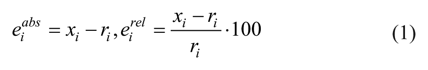
The BCN database we used was extracted from a larger database collected in a multicenter study conducted in 2014 (the original specific aim was to assess the accuracy of a CGM sensor).²⁴ For our purposes, the study involved 51 subjects (44 with T1D, 7 with T2D) who participated in a 12-hour clinical session in which BG concentration was monitored every 30 minutes by an SMBG device, the BCN, and every 15 minutes by YSI. A total of 1410 SMBG measurements were collected (on average 27 per subject). Similarly, to the OTU2 database, diet and insulin therapy were arranged to make BG vary in a wide range. Figure 1B shows a representative data set.

Methods

Preprocessing

Preprocessing of YSI and SMBG-YSI matching

To provide realizations of SMBG measurement error, required to develop a model of its PDF, each SMBG sample should be matched to a corresponding reference value, that is, ideally a YSI value collected at the same time. Unfortunately, both the databases we consider were originally collected to assess accuracy of CGM sensors, thus with a scope different from that of the present paper. For this reason, as visible in Figure 1, the SMBG data are in most cases not temporally aligned with the YSI samples. Consequently, the two measurements cannot be directly compared. To circumvent this problem, YSI sequences were preprocessed according to the following two-step procedure.

Figure 1.

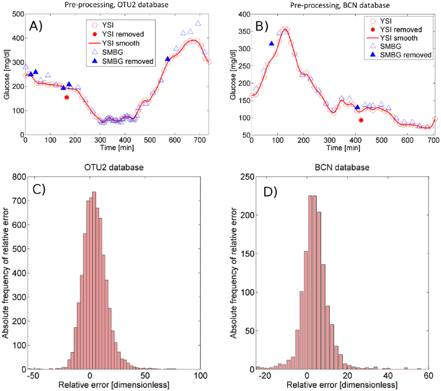
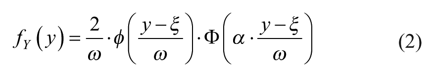
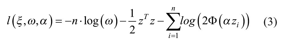
Panels A and B illustrate the preprocessing performed on a 12-hour YSI sequence of OTU2 and BCN database, respectively. The continuous line represents the quasi continuous-time smoothed profile obtained from YSI measurements (empty circles) after removing inaccurate samples (full circles). Triangles represent all available SMBG measurements. SMBG samples within YSI gaps are removed from the analysis (full triangles). Histograms (absolute frequencies) of the SMBG relative error in OTU2 and BCN database are reported in panels C and D, respectively.

First, YSI measurements considered not compatible with the BG pattern were removed from the analysis (see, eg, the full red circle in Figure 1, panels A and B). In particular, we adopted an empirical rule according to which an YSI sample is considered not compatible with the BG pattern if it deviates upward/downward more than a certain quantity θ from the previous and the following YSI samples, and the following YSI sample is in line with the previous YSI sample, that is, it does not deviate upward/downward more than ϵ from the previous YSI sample. More specifically, the jth YSI sample (empty red circles in Figure 1, panels A and B), YSI_j, is removed if YSI_j<YSI_j-1-θ(YSI_j-1), YSI_j<YSI_j+1-θ(YSI_j+1) and YSI_j+1>YSI_j-1-ϵ, or YSI_j>YSI_j-1+θ(YSI_j-1), YSI_j>YSI_j+1+θ(YSI_j+1) and YSI_j+1<YSI_j-1+ϵ. In particular, we set ϵ equal to 5 mg/dl and θ(x) equal to 15 mg/dl when x≤100 mg/dl, 15% x when x>100 mg/dl.

In the second step, from each 12-hour YSI sequence, an estimate of the BG profile was reconstructed on a quasi-continuous time grid by a nonparametric smoothing stochastic approach described in De Nicolao et al,²⁵ which allows to compensate the unavoidable presence of measurement error on YSI samples (zero-mean, uncorrelated and with constant coefficient of variation equal to 2%, according to the YSI 2300 STAT PLUS user’s manual).²⁶ Notably, as shown in De Nicolao et al,²⁵ the use of a maximum-likelihood smoothing criterion in this method limits the risk of introducing distortion/bias in the BG profile reconstructed from the YSI samples (as visible in the representative examples of Figure 1, panels A and B).

Samples (we chose a 1-min step) of the reconstructed BG profile (continuous line in Figure 1, panels A and B) were used as references for the calculation of SMBG measurement error. For such a scope, each SMBG sample (empty blue triangles in Figure 1, panels A and B) was matched to the nearest (in time) sample of the reconstructed BG profile (hence, the temporal distance between the SMBG sample and the reference sample is not greater than 30 sec).

Of note is that when one or more YSI samples are missing, and thus two consecutive YSI measurements are 30 min or more far from each other, the reconstruction of the BG profile over the gaps was considered not reliable and SMBG measurements falling inside these gaps were excluded from the analysis (full blue triangles in Figure 1, panels A and B). As a result, 4.37% and 3.05% of available SMBG measurements were excluded from the analysis, respectively for OTU2 and BCN database. Specifically, for OTU2 and BCN respectively, 20 and 4 SMBG samples were excluded in severe hypoglycemia (BG≤50 mg/dl), 13 and 4 in mid-hypoglycemia (50 mg/dl<BG≤70 mg/dl), 144 and 19 in euglycemia (70 mg/dl<BG<180 mg/dl), 66 and 8 in mid-hyperglycemia (180 mg/dl≤BG<250 mg/dl) and 59 and 8 in severe hyperglycemia (BG≥250 mg/dl).

Databases after preprocessing

After the preprocessing described in the previous subsection, the SMBG samples selected for the analysis resulted well distributed in the glycemic range, with a number of samples in hypoglycemia and hyperglycemia sufficiently high to allow an accurate description of SMBG measurement error also in these extreme conditions. In particular, the SMBG samples selected for the analysis were distributed in the glycemic range as follows: 356 (OTU2) and 123 (BCN) samples were in the severe hypoglycemia, 930 (OTU2) and 159 (BCN) in mid-hypoglycemia, 2958 (OTU2) and 463 (BCN) in euglycemia, 1479 (OTU2) and 399 (BCN) in mid-hyperglycemia, 881 (OTU2) and 222 (BCN) in severe hyperglycemia.

The obtained SMBG-BG matched pairs are used to calculate SMBG absolute and relative errors.

Absolute and relative error computation

For each SMBG sample in the training set ${x_{i}}$ , i = 1,…,n_tot (n_tot indicating the total number of SMBG measurements selected for the analysis in the preprocessing step) both absolute and relative (in percentage) errors are computed using the reference values ${r_{i}}$ , i = 1,…,n_tot:

e_{i}^{a b s} = x_{i} - r_{i}, e_{i}^{r e l} = \frac{x_{i} - r_{i}}{r_{i}} \cdot 100

Note that here we refer to absolute error and relative error as the signed difference and the signed percentage difference between the SMBG measurement and its reference sample.

In the bottom panels of Figure 1, the histogram of SMBG relative error is reported for OTU2 (panel C) and BCN database (panel D). Both meters present a unimodal, positively biased and skewed distribution. The BCN shows a significantly lower error variability than the OTU2. Note that the histogram of BCN error presents some outliers, that is, high values in the tails (eg, values lower than −10 and greater than 30 with significantly greater than zero absolute frequency). A possible way to describe the error PDF of data containing a significant number of outliers might be modeling the nonoutlier central part of the distribution separately from the outliers, as performed later in “Maximum-Likelihood Fitting.”

Model Development and Validation

To achieve the scope of delivering a model of the PDF of SMBG measurement error, two strategies are possible. The first is to resort to a parametric approach in which it is assumed that the PDF we want to describe presents a known shape characterized by a fixed, and usually small, number of parameters. The disadvantage is that it requires making some assumptions. The second possibility is to use nonparametric approaches, but coping with the risk of overfitting (ie, to include in the model phenomena related to the specific data set used only) can be difficult. Moreover, nonparametric methods do not allow to obtain any information on the PDF’s properties, in the specific they do not allow to establish if the distribution is unimodal, it presents a positive skewness, and so on.

Here, a parametric model of the SMBG error PDF is derived and validated in four steps: (1) creation of training and test set; (2) identification of BG zones of the training set in which the errors present a constant SD distribution; (3) maximum-likelihood (ML) fitting of a skew-normal PDF model to errors and an exponential PDF model to outliers in each identified zone of the training set; (4) model validation by assessing the mean absolute difference (MAD) between the empirical distribution function of random samples simulated by the model and the empirical distribution function of test set data and goodness-of-fit tests. Below these four steps are described in detail.

Creation of training and test set

Error data are divided into two parts. The first part, with cardinality n_training, is used as training set to derive the model of SMBG error PDF in the following steps B and C. The second part, with cardinality n_test, is used as test set to validate the model in step D. Absolute and relative errors of training set can be displayed in a scatterplot versus reference glucose to visually assess if the characteristics of error distribution (eg, mean and dispersion) significantly vary within the reference glucose range.

Constant SD zones identification

Changes in the dispersion of absolute and relative errors with reference glucose are quantified in the training set by analyzing the sample SD. In particular, first a uniform grid g_i i = 1,…,n_g, where n_g is the number of points in the grid, is defined in the glucose range with step S (eg, S = 5 mg/dl). Then, intervals centered at points g_i i = 1,…,n_g with half-width L (eg, L = 15 mg/dl) are defined. Finally, the sample SD of absolute and relative error samples in each interval g_i±L is calculated, which approximates the SD of error (absolute or relative) at the glucose point g_i. The plot of sample SD values versus glucose points g_i i = 1,…,n_g allows to analyze how the SD of error (absolute or relative) varies in the glucose range and identify zones of the glucose range in which either absolute or relative error presents approximately a constant SD distribution.

Maximum-likelihood fitting

In each constant SD zone, the distribution of the error (absolute or relative) in the training set, here represented by the continuous random variable Y, is fitted by ML using a certain PDF model. In particular, first, a Lilliefors test of normality is applied to error (absolute or relative) with significance level ρ. Then, if the Lilliefors test cannot reject the normality hypothesis, the Gaussian PDF model is used. Conversely, if the Lilliefors test rejects the normality hypothesis, the skew-normal PDF model is employed. The skew-normal PDF²⁷ is described by the following equation:

f_{Y} (y) = \frac{2}{ω} \cdot ϕ (\frac{y - ξ}{ω}) \cdot Φ (α \cdot \frac{y - ξ}{ω})

where $ϕ (\cdot)$ and $Φ (\cdot)$ are, respectively, the PDF and the cumulative distribution function of the standard Gaussian random variable, while the scalars ξ, ω, and α are, respectively, the location, scale, and skewness parameters of the skew-normal PDF. The skew-normal PDF model allows to describe both positively (α>0) or negatively (α<0) skewed PDF. When α is equal to zero, the skew-normal PDF becomes the Gaussian PDF.

Let us define $y = {[y_{1}, \dots, y_{n}]}^{T}$ as the vector of n samples of the error (absolute or relative), that is, n realizations of Y, falling within one of the identified constant SD glucose zones. Then, the parameters of the skew-normal PDF that best reproduces the distribution of data in y are estimated by maximizing the log-likelihood function:

l (ξ, ω, α) = - n \cdot \log (ω) - \frac{1}{2} z^{T} z - \sum_{i = 1}^{n} l o g (2 Φ (α z_{i}))

where $z_{i}$ , i = 1,…,n are the n components of $z = (y - ξ \cdot 1_{n}) / ω$ , with $1_{n}$ representing the nx1 unitary vector.

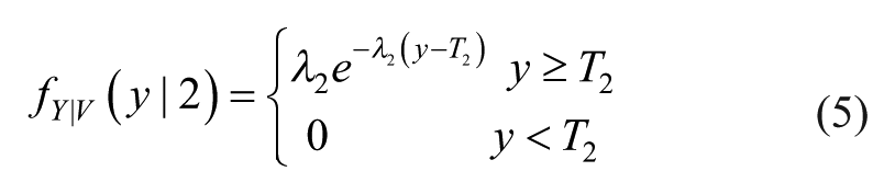
If the error (absolute or relative) distribution does not present a significant number of left or right outliers, that is, values in the left or right tails of the error histogram with significantly greater than zero frequency, the model of equation 2 should be sufficiently accurate to describe the error PDF. On the contrary, if the SMBG error presents nonnegligible left or right outliers, it should be more convenient to use a composite model in which the distributions of outliers and nonoutliers are described by different PDF models. Here, we propose a model obtained combining the skew-normal PDF and the exponential PDF. To derive such a model, two thresholds must be identified, T₁ and T₂, to separate the nonoutlier region, T₁≤y≤T₂, from the left outlier region, y<T₁, and the right outlier region, y>T₂. Let us define a discrete random variable V that can assume three values: 0, with probability p_V(0), when the SMBG error y is not an outlier; 1, with probability p_V(1), when y is a left outlier; 2, with probability p_V(2), when y is a right outlier. Then, the model defined for the PDF of Y, f_Y(y), is conditioned by the value of V. In particular, when V = 0 the conditional PDF of Y given V, f_Y|V(y|0), is the skew-normal PDF model of equation 2, whose parameters are identified by ML as described above. When V = 1, f_Y|V(y|1) is described by an exponential PDF model reversed with respect to the ordinate axis and shifted left of T₁:

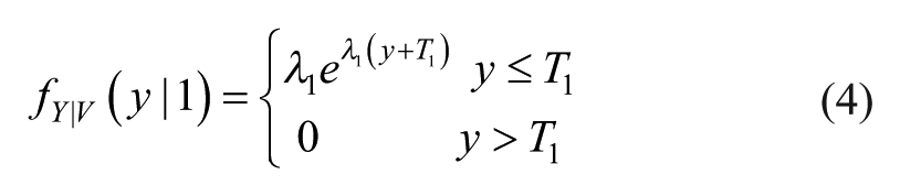
f_{Y | V} (y | 1) = {\begin{matrix} λ_{1} e^{λ_{1} (y + T_{1})} & y \leq T_{1} \\ 0 & y > T_{1} \end{matrix}

When V = 2, f_Y|V(y|2) is described by an exponential PDF model shifted right of T₂:

f_{Y | V} (y | 2) = {\begin{matrix} λ_{2} e^{- λ_{2} (y - T_{2})} & y \geq T_{2} \\ 0 & y < T_{2} \end{matrix}

Parameters λ₁ and λ₂ are estimated by ML by inverting the sample mean of left or right outliers properly shifted and reversed. Finally, the PDF of Y is obtained as:

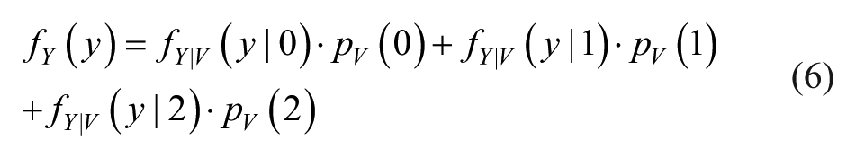
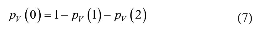
\begin{array}{l} f_{Y} (y) = f_{Y | V} (y | 0) \cdot p_{V} (0) + f_{Y | V} (y | 1) \cdot p_{V} (1) \\ + f_{Y | V} (y | 2) \cdot p_{V} (2) \end{array}

where the values p_V(1) and p_V(2) are estimated by dividing the number of observed left or right outliers for the total number of observed error values in the specific constant SD zone, while p_V(0) is found as:

p_{V} (0) = 1 - p_{V} (1) - p_{V} (2)

Remark. We propose for step C the use of canonical PDF models, like the skew-normal and the exponential, since they can be easily used to generate random samples in in silico applications. Conversely, the use of a noncanonical model, for example, a spline model, would require much more complex procedures to generate random samples from the model.

Validation

The model identified in each constant SD zone for absolute or relative error is validated by assessment of the MAD between the empirical distribution function of random samples simulated by the model and the empirical distribution function of test set data, and by application of two-sample Kolmogorov-Smirnov (KS) and Cramér-von Mises (CvM) goodness-of-fit tests. For such a purpose, M random samples are simulated by drawing n_test values from the model identified in each zone, being n_test the cardinality of the test set. In particular, SMBG error values are drawn from the exponential PDF of left outliers with probability p_V(1), from the exponential PDF of right outliers with probability p_V(2) and from the skew-normal PDF of nonoutliers with probability p_V(0). If the model does not include outliers’ description, then p_V(1) = p_V(2) = 0 and all the n_test SMBG error values are drawn from the skew-normal PDF. To sample a random number y from a skew-normal PDF, with generic parameters ξ, ω and α, a three step method is provided in Azzalini.²⁷ First, two values u₀ and u₁ having marginal PDF N(0,1) and correlation $δ = α / \sqrt{1 + α^{2}}$ are generated by sampling u₀ and r from independent N(0,1) random variables and defining $u_{1} = δ \cdot u_{0} + \sqrt{1 - δ^{2}} \cdot r$ . Then, in the second step, a random number z sampled from a skew-normal PDF with parameters ξ = 0, ω = 1 and α≠0 is obtained as:

z = {\begin{matrix} u_{1} & i f u_{0} \geq 0 \\ - u_{1} & o t h e r w i s e \end{matrix}

As third step, the realization sampled from the skew-normal PDF with parameters ξ, ω and α is finally obtained setting y = ξ+ωz.

For each of the M simulated samples, first the empirical distribution function (EDF) is calculated which represents an estimate of the cumulative distribution function. In particular, given a generic random sample, Y_j j = 1,…n, its EDF is defined as $\hat{F} (y) = \frac{1}{n} \sum_{j = 1}^{n} I_{[- \infty y]} (Y_{j}),$ where $I_{[- \infty y]}$ is 1 if Y_j≤0 and 0 otherwise. Then, the MAD between the EDF of each simulated sample and the EDF of the test set is calculated and its average value on the M simulated samples is obtained. Finally, each of the M simulated samples is compared to the test set error data by performing, with significance level β, the two-sample KS and CvM tests, that is, nonparametric tests for the null hypothesis H₀ = “the two samples are drawn from the same distribution” based on a measure of distance between the EDFs of the two samples. The percentage of simulated samples for which KS and CvM tests reject H₀ is calculated, that, if the identified model of SMBG error PDF is accurate, should be small.

This validation is performed N times (eg, N = 100), to avoid that the results of the validation can be dependent on the particular realization of random samples. Therefore, the average MAD and the percentage of samples for which KS and CvM tests reject H₀ are obtained for the N groups of M random samples and finally their mean, minimum and maximum values are calculated.

Results

For each SMBG sample, absolute and relative errors have been computed as described by equation 1. Then, the whole set of SMBG error data, with cardinality n_tot, was divided into a training set with cardinality n_training = 2/3·n_tot and a test set with cardinality n_test = 1/3·n_tot. The scatterplots of Figure 2 report, versus reference glucose values, absolute and relative errors in the training set, which result positively biased and with nonuniform dispersion over the entire reference glucose range for both OTU2 (panels A and B respectively) and BCN (panels C and D respectively).

Figure 2.

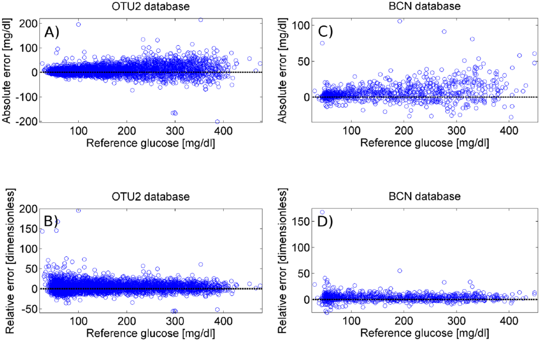
Scatterplots of absolute and relative error vs reference glucose for the training set of OTU2 (panels A and B, respectively) and BCN (panels C and D, respectively) database.

In Figure 3 the SD of absolute (top panels) and relative (bottom panels) error in the training set is displayed for increasing glucose values. In particular, the sample SD of absolute and relative error in the training set was computed on glucose intervals of half-width L = 15 mg/dl centered at the points of a glucose grid with uniform step S = 5 mg/dl. This representation allows to analyze how the SD of absolute and relative error varies in the glucose range. For the OTU2: the SD of absolute error (panel A) is approximately constant for glucose values lower than 75 mg/dl, while an increasing trend is observed for glucose values greater than 75 mg/dl; conversely, the SD of relative error (panel B) presents a decreasing trend for glucose values lower than 75 mg/dl, while appearing approximately constant for glucose values greater than 75 mg/dl. Therefore, two constant SD zones were identified: zone 1, that is, BG≤75 mg/dl, with constant SD absolute error; zone 2, that is, BG>75 mg/dl, with constant SD relative error. For BCN, the SD of absolute and relative error in the training set is reported respectively in panel C and D. Again, two zones are identified: zone 1, that is, BG≤115 mg/dl, with constant SD absolute error; zone 2, that is, BG >115 mg/dl, with constant SD relative error. Note that, for both the OTU2 and the BCN database, the absolute or relative error in zones 1 and 2 is not correlated with the reference BG, as visible in the scatterplots of Figure 2.

Figure 3.

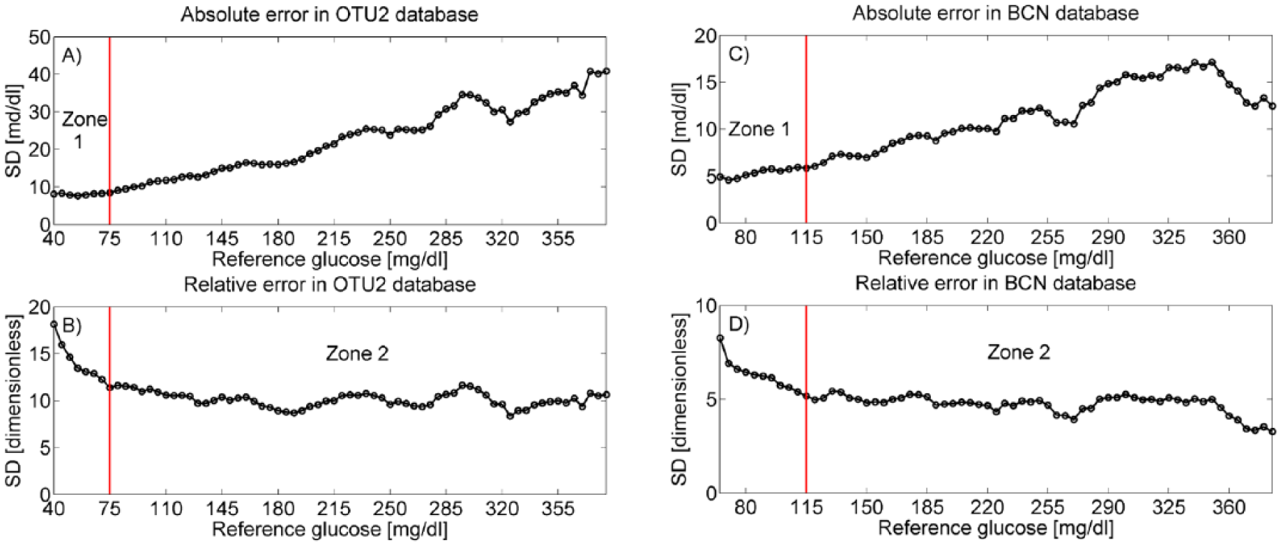
Absolute and relative error SD vs reference glucose for the training set of OTU2 (panels A and B, respectively) and BCN (panels C and D, respectively) database. The thresholds to separate zone 1 from zone 2 (75 mg/dl in OTU2 database, 115 mg/dl in BCN) are evidenced by vertical red lines.

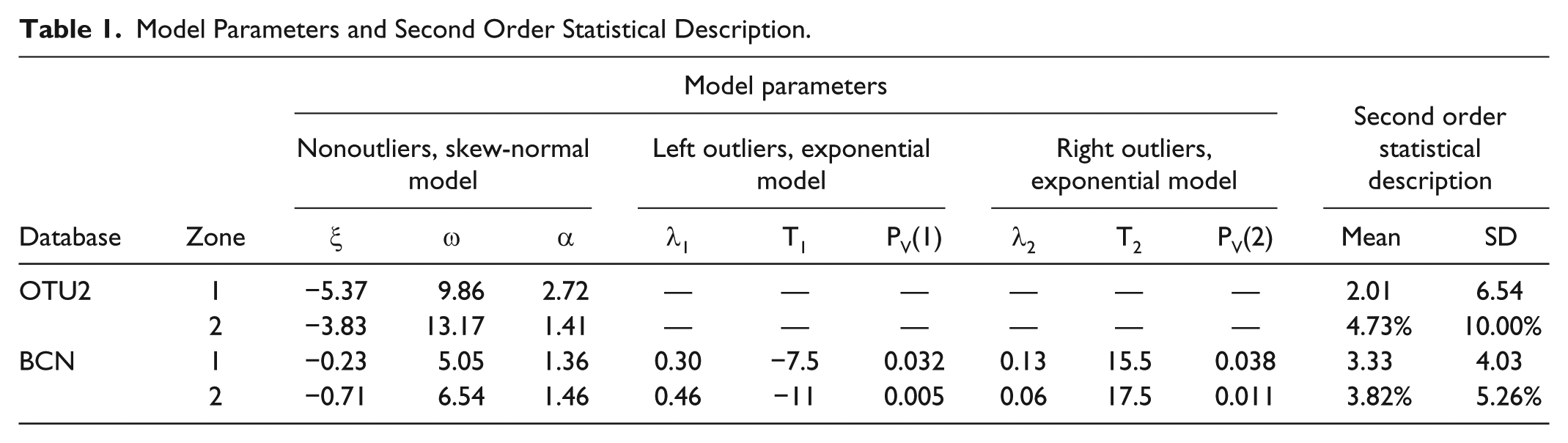
The histograms of Figure 4 represent the relative frequency of absolute (top panels) and relative (bottom panels) error, calculated in the training set, in zones 1 (left panels) and 2 (right panels). For both databases, the Lilliefors test rejected the normality hypothesis for the absolute error in zone 1 and the relative error in zone 2, using as significance level ρ = 5% (P = .001). This result suggests that a Gaussian PDF model would not be a proper model to accurately describe the observed SMBG error distribution. For OTU2, since the error distributions in zone 1 and 2 do not show a significant number of outliers, a simple skew-normal PDF model (black line) was fitted by ML both in zone 1 (panel A) and 2 (panel B). Indeed, in this database the skew-normal model alone is sufficient to well fit both the central part and the tails of the SMBG error distribution (as witnessed by Figure 4, panels A and B), while the use of exponential distributions did not improve the data fit (not shown). In Table 1, the values of location, scale and skewness parameters, mean and SD are reported for the identified models in zone 1 and 2. In particular, both error models present a significant positive mean (2.01 mg/dl in zone 1, 4.69% in zone 2) and positive skewness (α = 2.76 in zone 1 and α = 1.43 in zone 2). For BCN, some outliers are visible in the error distribution of training set data both in zone 1 (panel C) and 2 (panel D). In particular, in zone 1 values lower than -7.5 mg/dl were considered left outliers and values greater than 15.5 mg/dl were considered right outliers, while in zone 2 we considered left outliers values under -11%, right outliers values over 17.5%. The values for thresholds T₁ and T₂, which are also reported in Table 1, were determined by a commonly used definition of outliers: T₁ = Q₁-1.5·(Q₃-Q₁) and T₂ = Q₃+1.5·(Q₃-Q₁), where Q₁ and Q₃ represent the first and the third quartiles, respectively. Left and right outliers’ distributions were fitted by the exponential PDF models of equations 4 and 5, while nonoutliers’ distribution was fitted by the skew-normal PDF of equation 2. The parameters of the identified models are reported in Table 1 (last two rows). Panels C and D of Figure 4 show how the composite PDF obtained by equation 6 (black line) well approximates the error distribution of training set data respectively in zone 1 and 2.

Figure 4.

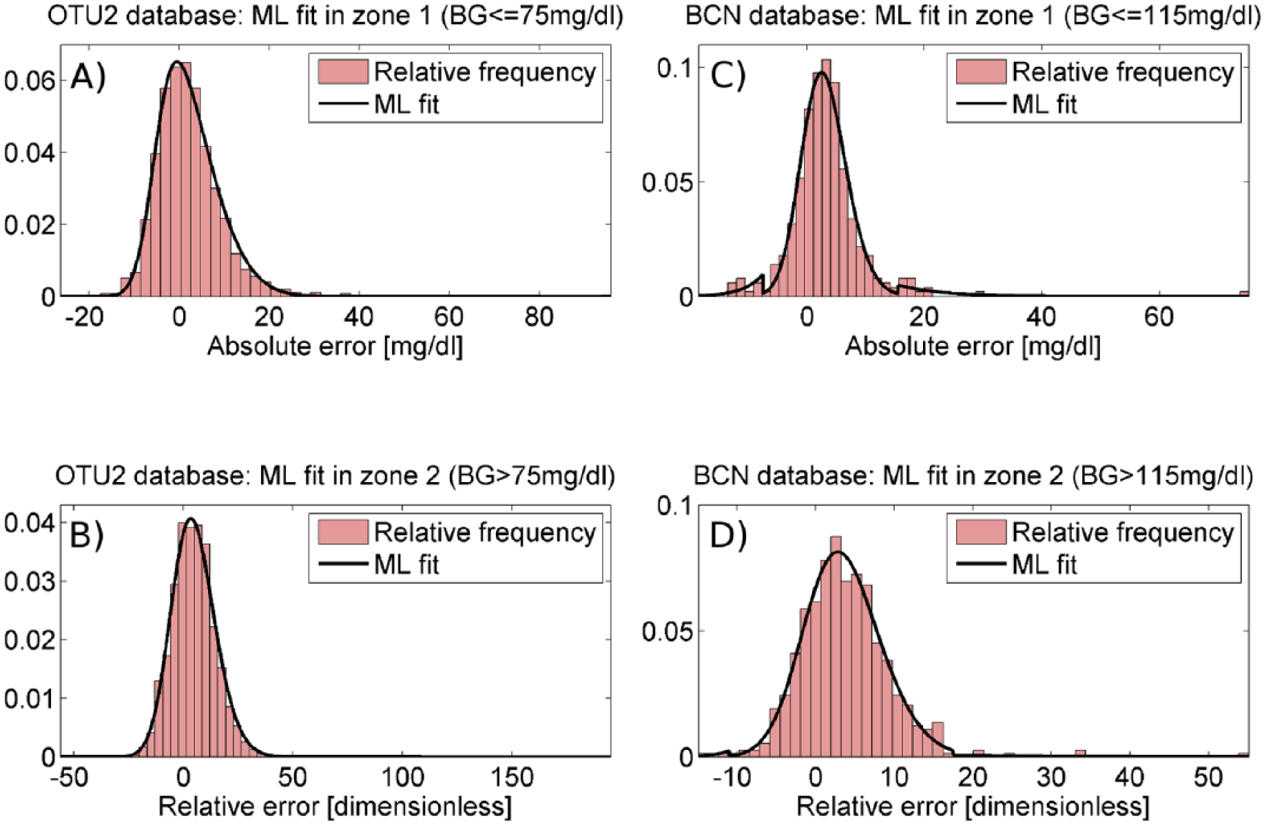
Panels A and B report the ML fit of the skew-normal PDF (black line) against histograms of, respectively, absolute and relative error (red bars) in zone 1 and 2 of the training set of OTU2 database. Panel C and D report the ML fit of the PDF model obtained as combination of the skew-normal and the exponential PDF (black line) against histograms of, respectively, absolute and relative error (red bars) in zone 1 and 2 of the training set of BCN database.

Table 1.

Model Parameters and Second Order Statistical Description.

Database	Zone	Model parameters									Second order statistical description
		Nonoutliers, skew-normal model			Left outliers, exponential model			Right outliers, exponential model			Second order statistical description
		ξ	ω	α	λ₁	T₁	P_V(1)	λ₂	T₂	P_V(2)	Mean	SD
OTU2	1	−5.37	9.86	2.72	—	—	—	—	—	—	2.01	6.54
OTU2	2	−3.83	13.17	1.41	—	—	—	—	—	—	4.73%	10.00%
BCN	1	−0.23	5.05	1.36	0.30	−7.5	0.032	0.13	15.5	0.038	3.33	4.03
BCN	2	−0.71	6.54	1.46	0.46	−11	0.005	0.06	17.5	0.011	3.82%	5.26%

For validation purposes, the identified PDF model was used to generate, for each zone, N = 100 groups of M = 500 random samples having cardinality equal to the number of error data available in the test set for the same glucose zone. As visible in Figure 5, the EDFs of random samples simulated by the identified PDF model (blue solid lines) are very similar to the EDF calculated for test set data (red solid line) both in zone 1 and 2 of OTU2 (panels A and B, respectively) and BCN database (panels C and D, respectively). In particular, the mean, minimum and maximum values of average MAD between the EDF of simulated data sets and the EDF of test set data, obtained in the 100 groups of 500 simulated random samples, are reported in Table 2 for the two databases (second and third column). Two-sample KS and CvM tests are performed with significance level β = 5% on the 100 groups each containing 500 simulated random samples. In OTU2 database, on average, the KS test rejects H₀ for the 0.53% (0.00%-1.40%) of zone 1 simulated samples and the 1.94% (0.40%-4.6%) of zone 2 simulated samples, while the CvM test rejects H₀ for the 0.94% (0.00%-2.20%) of zone 1 simulated samples and the 4.15% (1.40%-6.60%) of zone 2 simulated samples. In BCN database, on average, the KS test rejects H₀ for the 0.75% (0.00%-1.80%) and 1.43% (0.40%-2.60%) of zone 1 and 2 simulated samples, respectively, while the CvM test rejects H₀ for the 0.95% (0.20%-2.20%) and 2.56% (1.40%-4.00%) of zone 1 and 2 simulated samples, respectively. Since, for almost all the simulated random samples, H₀ cannot be rejected and the MAD between the EDF of simulated samples and test set data result small (Table 2), we can conclude that the two-zone skew-normal models derived for OTU2 and BCN well reproduce the SMBG error distribution observed in the test set.

Figure 5.

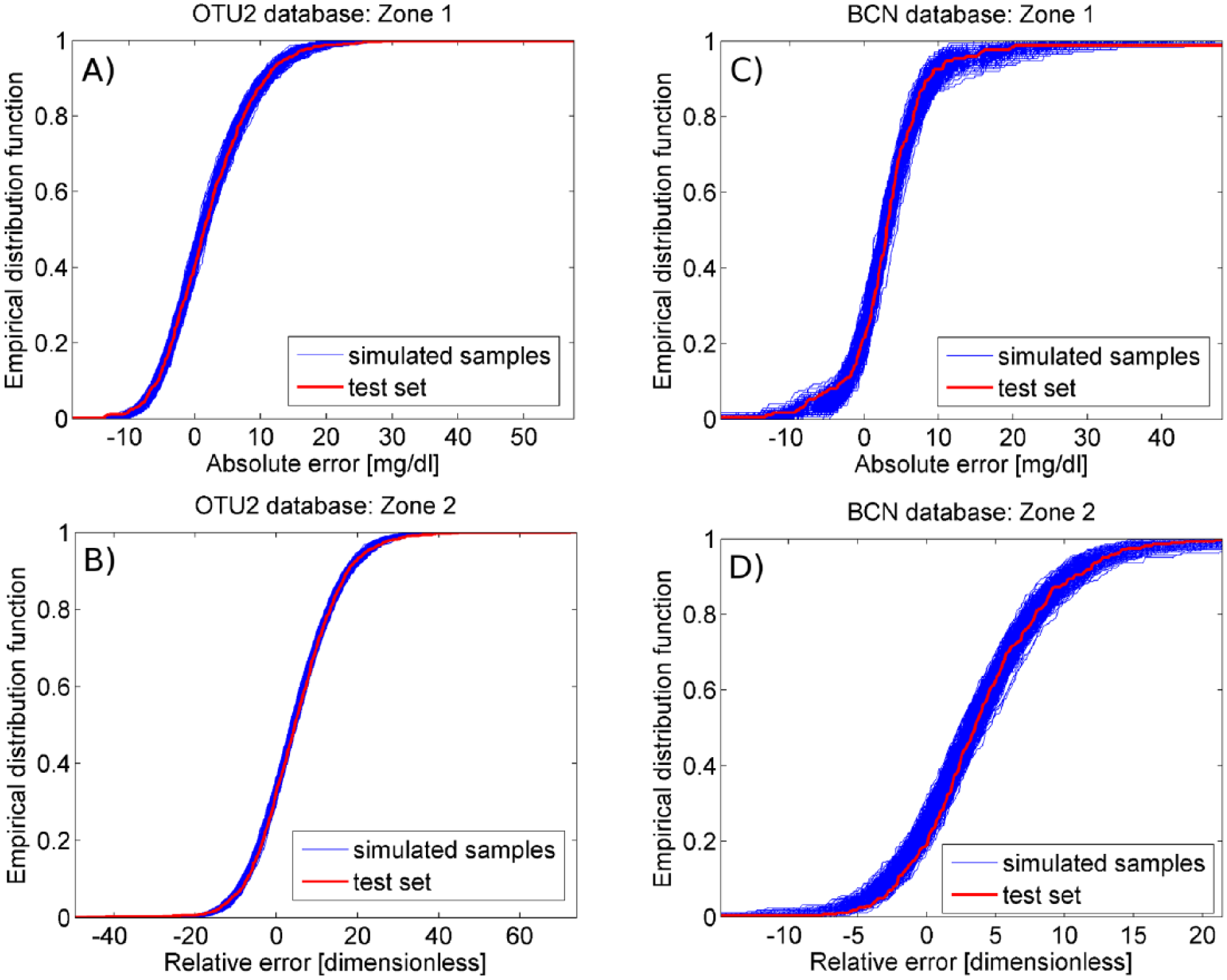
The empirical distribution function of simulated random samples (blue line) and test set data (red line) is reported for zone 1 and 2 of OTU2 database (panels A and B, respectively) and BCN database (panels C and D, respectively).

Table 2.

Mean (Minimum-Maximum) of the Average MAD Between 500 Simulated EDFs and Test Set EDF.

Database	Two-zone skew-normal model		Two-zone Gaussian model		Single-zone Gaussian model
Database	Zone 1	Zone 2	Zone 1	Zone 2	Single-zone Gaussian model
OTU2	0.0064 (0.0062-0.0065)	0.0049 (0.0048-0.0050)	0.0172 (0.0170-0.0175)	0.0079 (0.0077-0.0079)	0.0115 (0.0114-0.0116)
BCN	0.0131 (0.0128-0.0134)	0.0156 (0.0150-0.0161)	0.0296 (0.0292-0.0301)	0.0270 (0.0264-0.0275)	0.0393 (0.0391-0.0397)

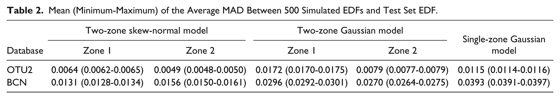
MAD and two-sample KS and CvM tests also demonstrate that the identified two-zone skew-normal models outperform simpler Gaussian models like the single-zone Gaussian model, previously used in the literature to describe SMBG relative error distribution,^11-13 and the two-zone Gaussian model in which a Gaussian (instead of skew-normal and exponential) PDF is used to describe absolute error in zone 1 and relative error in zone 2. Indeed, when the single-zone Gaussian model is used, the mean of average MAD (reported in the sixth column of Table 2) is about twice, in the OTU2 database, and three times, in the BCN database, the mean of average MAD obtained with the two-zone skew-normal model. In addition, the two goodness-of-fit tests reject H₀ for almost the 100% of simulated samples (on average, the KS test rejects H₀ for the 99.44% in OTU2 database and 100.00% in BCN database, while the CvM test rejects H₀ for the 99.85% in OTU2 database and 100.00% in BCN database). When the two-zone Gaussian model is used, the mean of average MAD is about double the value obtained by the two-zone skew-normal model both in OTU2 and BCN databases, and H₀ is rejected for about 50% of zone 1 simulated samples or more (on average: 49.80%, for KS, and 70.00%, CvM, in OTU2 database; 59.21%, for KS, and 81.63%, for CvM, in BCN database) and more than 10% of zone 2 simulated samples (on average: 27.06%, for KS, and 24.03%, CvM, in OTU2 database; 14.20%, for KS, and 20.67%, for CvM, in BCN database).

Remark 1

The sparseness of SMBG data (4-5 samples per day) suggests assuming that measurement errors can be considered uncorrelated. To support reliability of this hypothesis, we evaluated, a posteriori, the autocorrelation function for each SMBG error sequence (both absolute and relative) corresponding to a specific subject. Results show that, for both absolute and relative error, in both OUT2 and BCN databases, the coefficients of the mean normalized autocorrelation function never overtake 0.5, confirming that uncorrelation of errors seems a reasonable assumption. Of course, a more detailed and precise assessment of the autocorrelation of the SMBG measurement error would require a separate study, with scope different from that of the present paper and, remarkably, ad hoc data sets consisting of SMBG measurements frequently collected in parallel to high accuracy BG reference samples.

Remark 2

The threshold dividing the two constant SD zones was 75 mg/dl for OTU2 and 115 mg/dl for BCN. These results are, not surprisingly, coherent with the requirements (in terms of accuracy) imposed to SMBG devices by the standard ISO 15197. Indeed, the 2003 standard²⁸ requires that 95% of the SMBG values should have an absolute error lower than 15 mg/dl for glucose concentration lower than 75 mg/dl and a relative error lower than 20% in the rest of the range, while the 2013 standard²⁹ requires that 95% of the SMBG values should have an absolute error lower than 15 mg/dl for glucose concentration lower than 100 mg/dl and a relative error lower than 15% in the rest of the range. In particular, the 75 mg/dl threshold we found for OTU2, which was approved by FDA in 2006, reflects the same partition defined by standard ISO 15197:2003, while the 115 mg/dl threshold we found for BCN, which was approved by FDA in 2012, is similar to the one defined by the standard ISO 15197:2013.

Discussion

A methodology to derive a model of the PDF of the SMBG measurement error has been proposed and tested on two different databases. The main novelties are the multizone approach, which consists in dividing the glucose range into zones with constant SD absolute or relative error, and the skew-normal PDF model, fitted in each identified zone, which allows to describe both symmetric and asymmetric PDF. The distribution of outliers, possibly present in the data, is described by an exponential PDF identified separately. In identifying model parameters, the unavoidable measurement error affecting references (YSI samples) is mitigated by the use of a well-established stochastic smoothing technique.

In both the OTU2 and the BCN databases, two zones were identified: a low glucose range (zone 1) with constant SD absolute error and a high glucose range (zone 2) with constant SD relative error. With regard to the distribution of the error in the two zones, absolute and relative errors respectively in zone 1 and 2 show a significantly positive mean for both the SMBG meters, while a significantly lower SD was observed for BCN in both zone 1 and 2. For OTU2, a simple skew-normal PDF model was identified for absolute and relative errors respectively in zone 1 and 2. For BCN, because of the presence of outliers in the error distribution, we identified, in both zone 1 and 2, a composite PDF model combining a skew-normal PDF and exponential PDF to describe respectively nonoutliers and outliers distributions. Notably, in modeling the PDF of measurement error, the presence of outliers cannot be neglected and should be explicitly taken into account. Indeed, outliers represent the less accurate SMBG measurements which may drive to incorrect treatment decisions and, thus, dangerous clinical consequences. Modeling such outliers, as done in our work, could be particularly important for in silico studies assessing the safety of SMBG-based insulin therapies, to understand their clinical impact on glycemic control.

From a practical perspective, it is useful remarking that the SMBG error models identified for OTU2 and BCN are credible over all the glycemic range, because the used experimental data included a sufficiently high number of SMBG samples (and matched BG references) in all the regions of the glycemic range (including severe hyperglycemia and severe hypoglycemia).

Validation by MAD of EDF and KS and CvM goodness-of-fit tests showed that the two PDF models well reproduce the data in both the considered databases, performing significantly better than the single-zone Gaussian model, used previously in the literature, and the two-zone Gaussian model.

Conclusion

We proposed a methodology to derive models of the PDF of SMBG measurement error. Application of the methodology to two real databases evidences, in particular, that SMBG devices present constant-SD absolute error in the low glucose range and constant-SD relative error in the high glucose. It could be interesting noting that this behavior for experimental data can be observed not only in analytical chemistry,³⁰ but also in other fields like, for example, in the case of gene expression arrays measurement error,³¹ and it is commonly taken into account by the standards defining the maximum allowable error of a measurement. For example, in the case of SMBG, the ISO 15197:2013 standard requires that the 95% of the SMBG measurements have absolute error lower than 15 mg/dl, for glucose concentrations below 100 mg/dl, and relative error lower than 15% in the rest of the glucose range. Conversely, a recent FDA guidance³² does not take into account the fact SMBG measurements may present a constant-SD absolute error at low glucose values (which is the case of the two devices investigated in this paper), and requires SMBG measurements to deviate no more than 15% from the reference BG values. As a consequence, this guidance imposes a stricter criterion to determine if an SMBG device is sufficiently accurate and, thus, not all the SMBG devices currently in the market may be able to meet this criterion at low glucose concentrations (see for example the scatterplots in Figure 2, panels B and D).

To conclude, we would like to report some remarks. First, the performance of the models derived by the proposed methodology was compared to simpler models based on the Gaussian distribution, commonly used in the literature. Of course, as a further development of the work presented in this paper, it would be interesting to compare the performance of our model to other possible PDF models (both parametric and nonparametric). Second, the proposed methodology has been applied in this paper to OTU2 and BCN databases, but it is of general usability and can be easily implemented to analyze whatever databases containing SMBG samples and matched BG references (unfortunately, at present time no other SMBG databases are available to us to further apply the method). Third, the models of the PDF of SMBG measurement error developed by the present methodology are of straightforward application in several in silico studies of clinical interest. In particular, a model of the PDF of the SMBG measurement error is a key component of models of T1D patient decision-making,³³ that is, a simulation framework that allows to create reliable in silico clinical trials to test the safety and effectiveness of insulin treatment scenarios, like the nonadjunctive use of CGM that was evaluated in an Advisory Panel meeting recently conducted by FDA.^3,4 Finally, the SMBG measurement error models we derived can be employed for several other in silico studies, for example to assess the influence of SMBG accuracy on algorithms for SMBG-based insulin dosing,³⁴ CGM calibration and optimization of the frequency of BG monitoring.³⁵

Footnotes

Acknowledgements

Dexcom, Inc (San Diego, CA) is acknowledged for having generously provided the data already published in Christiansen et al²³ and Bailey et al.²⁴

Abbreviations

BCN, Bayer Contour Next USB; BG, blood glucose; CGM, continuous glucose monitoring; CvM, Cramér-von Mises; EDF, empirical distribution function; FDA, Food and Drug Administration; ISO, International Standard for Standardization; KS, Kolmogorov-Smirnov; MAD, mean absolute difference; ML, maximum likelihood; OTU2, One Touch Ultra 2; PDF, probability density function; SD, standard deviation; SMBG, self-monitoring of blood glucose; T1D, type 1 diabetes; YSI, Yellow Spring Instruments.

Declaration of Conflicting Interests

The author(s) declared no potential conflicts of interest with respect to the research, authorship, and/or publication of this article.

Funding

The author(s) received no financial support for the research, authorship, and/or publication of this article.

References

Benjamin

EM.

Self-monitoring of blood glucose: the basics. Clin Diabetes. 2002;20(1):45-47.

Juvenile Diabetes Research Foundation Continuous Glucose Monitoring Study Group. Continuous glucose monitoring and intensive treatment of type 1 diabetes. N Engl J Med. 2008;359(14):1464-1476.

FDA Advisory panel votes to recommend non-adjunctive use of Dexcom G5 Mobile CGM. Diabetes Technol Ther. 2016;18(8):512-516.

Edelman

SV.

Regulation catches up to reality: nonadjunctive use of continuous glucose monitoring data. J Diabetes Sci Technol. 2016;11(1):160-164.

Facchinetti

Del Favero

Sparacino

Cobelli

Model of glucose sensor error components: identification and assessment for new Dexcom G4 generation devices. Med Biol Eng Comput. 2015;53(12):1259-1269.

Dalla Man

Micheletto

Breton

Kovatchev

Cobelli

The UVA/PADOVA type 1 diabetes simulator: new features. J Diabetes Sci Technol. 2014;8(1):26-34.

Breton

Kovatchev

BP.

Analysis, modeling, and simulation of the accuracy of continuous glucose sensors. J Diabetes Sci Technol. 2008;2(5):853-862.

Lunn

Wei

Hovorka

Fitting dynamic models with forcing functions: application to continuous glucose monitoring in insulin therapy. Stat Med. 2011;30(18):2234-2250.

Facchinetti

Del Favero

Sparacino

Castle

Ward

Cobelli

Modeling the glucose sensor error. IEEE Trans Biomed Eng. 2014;61(3):620-629.

10.

Laguna

Rossetti

Ampudia-Blasco

Vehi

Bondia

Postprandial performance of Dexcom® SEVEN® PLUS and Medtronic® Paradigm® VeoTM: modeling and statistical analysis. Biomed Signal Process Control. 2014;10:322-331.

11.

Boyd

Bruns

DE.

Quality specifications for glucose meters: assessment by simulation modelling of errors in insulin dose. Clin Chem. 2001;47(2):209-214.

12.

Boyd

Bruns

DE.

Monte Carlo simulation in establishing analytical quality requirements for clinical laboratory tests: meeting clinical needs. Methods Enzymol. 2009;467:411-433.

13.

Virdi

Mahoney

JJ.

Importance of blood glucose meter and carbohydrate estimation accuracy. J Diabetes Sci Technol. 2012;4(4):921-926.

14.

Freckmann

Baumstark

Jendrike

. System accuracy evaluation of 27 blood glucose monitoring systems according to DIN EN ISO 15197. Diabetes Technol Ther. 2010;12(3):221-231.

15.

Freckmann

Schmid

Baumstark

Pleus

Link

Haug

System evaluation of 43 blood glucose monitoring systems for self-monitoring of blood glucose according to DIN EN ISO 15197. J Diabetes Sci Technol. 2012;6(5):1060-1075.

16.

Freckmann

Baumstark

Schmid

Pleus

Link

Haug

Evaluation of 12 glucose monitoring systems for self-testing: system accuracy and measurement reproducibility. Diabetes Technol Ther. 2014;16(2):113-122.

17.

Breton

Kovatchev

BP.

Impact of blood glucose self-monitoring errors on glucose variability, risk for hypoglycaemia, and average glucose control in type 1 diabetes: an in silico study. J Diabetes Sci Technol. 2010;4(3):562-570.

18.

Karon

Boyd

Klee

GG.

Glucose meter performance criteria for tight glycemic control estimated by simulation modelling. Clin Chem. 2010;56(7):1091-1097.

19.

Karon

Boyd

Klee

GG.

Empiric validation of simulation models for estimating glucose meter performance criteria for moderate levels of glycemic control. Diabetes Technol Ther. 2013;15(12):996-1003.

20.

Pretty

Signal

Fisk

. Impact of sensor and measurement timing errors on model-based insulin sensitivity. Comput Methods Programs Biomed. 2014;114(3):e79-e86.

21.

Chan

JCN

Wong

Cheung

. Accuracy, precision and user-acceptability of self blood glucose monitoring machines. Diabetes Res Clin Pract. 1997;36(2):91-104.

22.

Vettoretti

Facchinetti

Sparacino

Cobelli

Accuracy of devices for self-monitoring of blood glucose: a stochastic error model. Conf Proc IEEE Eng Med Biol Soc. 2015;2015:2359-2362.

23.

Christiansen

Bailey

Watkins

. A new-generation continuous glucose monitoring system: improved accuracy and reliability compared with a previous-generation system. Diabetes Technol Ther. 2013;15(10):1-8.

24.

Bailey

Chang

Christiansen

Clinical accuracy of a continuous glucose monitoring system with an advanced algorithm. J Diabetes Sci Technol. 2015;9(2):209-214.

25.

De Nicolao

Sparacino

Cobelli

. Nonparametric input estimation in physiological systems: problems, methods and case studies. Automatica. 1997;33(5):851-870.

26.

User’s manual YSI 2300 STAT PLUS. Available at: https://www.ysi.com/File%20Library/Documents/Manuals%20for%20Discontinued%20Products/YSI-2300-Stat-Plus-manual-j.pdf.

27.

Azzalini

The skew-normal distribution and related multivariate families. Scand J Statist. 2005;32(2):159-188.

28.

International Organization for Standardization. ISO 15197:2003: In vitro diagnostic test systems—requirements for blood-glucose monitoring systems for self-testing in managing diabetes mellitus. Geneva, Switzerland: International Organization for Standardization; 2003.

29.

International Organization for Standardization. ISO 15197:2013. In vitro diagnostic test systems—requirements for blood-glucose monitoring systems for self-testing in managing diabetes mellitus. Geneva, Switzerland: International Organization for Standardization; 2013.

30.

Rocke

Lorenzato

A two-component model for measurement error in analytical chemistry. Technometrics. 1995;37(2):176-184.

31.

Rocke

Durbin

A model for measurement error for gene expression arrays. J Comp Biol. 2001;8(6):557-569.

32.

US Food and Drug Administration. Self-monitoring blood glucose test systems for over-the-counter use. 2016. Available at: http://www.fda.gov/downloads/medicaldevices/deviceregulationandguidance/guidancedocuments/ucm380327.pdf.

33.

Vettoretti

Facchinetti

Sparacino

Cobelli

Patient decision-making of CGM sensor driven insulin therapies in type 1 diabetes: in silico assessment. Conf Proc IEEE Eng Med Biol Soc. 2015;2015:2363-2366.

34.

García-Jaramillo

Calm

Bondia

Tarín

Vehí

Insulin dosage optimization based on prediction of postprandial glucose excursions under uncertain parameters and food intake. Comput Methods Programs Biomed. 2012;105(1):61-69.

35.

Wang

Paranjape

A signal processing application for evaluating self-monitoring blood glucose strategies in a software agent model. Comput Methods Programs Biomed. 2015;120(2):77-87.

A Model of Self-Monitoring Blood Glucose Measurement Error

Abstract

Background:

Methods:

Results:

Conclusions:

Keywords

Database

OTU2 Database

BCN Database

Methods

Preprocessing

Preprocessing of YSI and SMBG-YSI matching

Databases after preprocessing

Absolute and relative error computation

Model Development and Validation

Creation of training and test set

Constant SD zones identification

Maximum-likelihood fitting

Validation

Results

Remark 1

Remark 2

Discussion

Conclusion

Footnotes

Acknowledgements

Abbreviations

Declaration of Conflicting Interests

Funding

References