A Computational Proof of Concept of a Machine-Intelligent Artificial Pancreas Using Lyapunov Stability and Differential Game Theory

Abstract

Background:

This study demonstrated the novel application of a “machine-intelligent” mathematical structure, combining differential game theory and Lyapunov-based control theory, to the artificial pancreas to handle dynamic uncertainties.

Methods:

Realistic type 1 diabetes (T1D) models from the literature were combined into a composite system. Using a mixture of “black box” simulations and actual data from diabetic medical histories, realistic sets of diabetic time series were constructed for blood glucose (BG), interstitial fluid glucose, infused insulin, meal estimates, and sometimes plasma insulin assays. The problem of underdetermined parameters was side stepped by applying a variant of a genetic algorithm to partial information, whereby multiple candidate-personalized models were constructed and then rigorously tested using further data. These formed a “dynamic envelope” of trajectories in state space, where each trajectory was generated by a hypothesis on the hidden T1D system dynamics. This dynamic envelope was then culled to a reduced form to cover observed dynamic behavior. A machine-intelligent autonomous algorithm then implemented game theory to construct real-time insulin infusion strategies, based on the flow of these trajectories through state space and their interactions with hypoglycemic or near-hyperglycemic states.

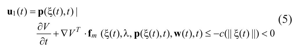
Results:

This technique was tested on 2 simulated participants over a total of fifty-five 24-hour days, with no hypoglycemic or hyperglycemic events, despite significant uncertainties from using actual diabetic meal histories with 10-minute warnings. In the main case studies, BG was steered within the desired target set for 99.8% of a 16-hour daily assessment period. Tests confirmed algorithm robustness for ±25% carbohydrate error. For over 99% of the overall 55-day simulation period, either formal controller stability was achieved to the desired target or else the trajectory was within the desired target.

Conclusions:

These results suggest that this is a stable, high-confidence way to generate closed-loop insulin infusion strategies.

In the treatment of type 1 diabetes (T1D), perhaps the most useful innovation short of a cure would be an effective “artificial pancreas” (AP), enabling stable, closed-loop infused insulin in response to both the ongoing dynamics of T1D glucose-insulin homeostasis and the ongoing external perturbations of meals, exercise, sleep, and menstruation, among others. In this article, it is argued that existing medical devices can provide a significantly better quality of blood glucose (BG) control through the exploitation of alternative mathematical methods coupled with the availability of computing resources in cloud and mobile platforms.

The mathematical approach demonstrated here, a combination of differential game theory and Lyapunov stability theory, obtained much of its background theory in robotics. Industrial robots typically have highly nonlinear, coupled dynamics of high dimension and significant dynamic uncertainties, while only a small number of variables are observable in (noise-polluted) time series. Furthermore, robotic systems typically degrade over time due to selective wear in mechanisms, generating idiosyncratic dynamic behavior. From the late 1970s to early 1990s, a group of researchers in robotic controls rejected “classic” identification and controller techniques (model linearization, dynamic optimization) partly because these were incompatible with robust handling of the nonlinear dynamic uncertainties for ongoing control of the system using noise-polluted partial information.

Instead, Lyapunov-based methods were developed for nonlinear identification, nonlinear controllers, and nonlinear Model Reference Adaptive Control (MRAC)—the implementation of which was described compendiously as the Product State Space Technique (PSST)^1-8—in a body of robotics research that has more recently enjoyed a revival.^{9 -13} This provided the genesis of a medical platform technology^14,15 demonstrated here in an AP context.

In 2002, Greenwood ¹⁴ outlined a “control-to-range” mathematical method for steering the solution trajectories of a biological dynamic system to a specified target range or more complicated set, using incomplete information, despite the existence of significant uncertainties or uncontrolled elements in the system dynamics. This was done using differential game theory, inspired by earlier nonbiological works.^16,17 One or more Lyapunov functions were to be used to describe controller objectives in terms of steering solution trajectories to a target set sandwiched between nested contours of a Lyapunov function. Uncertainties or uncontrolled elements were to be ascribed to a hostile player (“Nature”), who would endeavor to prevent those trajectories from colliding with or being captured by the target. A minimax method was described, applied to distinct variables controlled by these mutually hostile players, to generate a control program robust to real-world uncertain dynamic elements.

Important differences exist between this approach and other published applications of robust control methods to the AP problem, which also typically use a minimax approach to uncertainties. Two examples are those of Parker et al ¹⁸ and Kovács et al, ¹⁹ who have employed modified forms of Sorenson’s ²⁰ model (rather than the usual T1D benchmark model of Dalla Man et al ²¹ and Magni et al ²² ; Sorenson, ²⁰ Dalla Man et al, ²¹ and Magni et al ²² represent nonlinear models of T1D glucose-insulin homeostasis); Parker et al ¹⁸ applied an implementation of the H∞ control, while Kovács et al ¹⁹ applied a Linear Parameter Varying (LPV) model–based control algorithm, itself an extension of linear time-invariant systems.

An important criticism of both examples’ approaches is that they have necessarily involved significant linearization of the model: for instance, Parker et al ¹⁸ linearized the model and reduced it to a third-order linear form for controller synthesis, while the method of Kovács et al ¹⁹ involved the construction of a polytopic region with the model built up by a linear combination of the linearized models derived in each polytopic point.

A problem with significant linearization of nonlinear glucose-insulin dynamics is that it introduces two layers of potential instability in the control algorithm:

1. The first layer is due to the discrepancy between the nonlinearized and linearized models, which can be compensated within a specified domain using rigorous simulation testing.

2. The second layer is fundamental: all mathematical models of glucose-insulin homeostasis and the insulin-based control are themselves only approximations of biological reality. Even in sophisticated models such as that of Magni et al, ²² some processes typically assumed to have a fixed linear structure can be reasonably expected to be, in reality, significantly nonlinear and/or time varying. Examples include the individualized, time-dependent nature of insulin sensitivity in T1D ²³ and the nonlinearity of insulin infusion pharmacokinetics (PK) (see Kraegen and Chisholm, ²⁴ who attempted to fit linear parameters and found these values to be dependent on the infusion profile, suggesting “that the linear model is an oversimplification”). Given that specific forms of such unmodeled nonlinearities are typically unknown a priori, it is difficult to be confident in the stability of control laws reliant on linearized models.

This criticism, and associated problems with nonlinear identification and nonlinear state observers, was overcome in the present study through the use of Lyapunov functions and differential game theory, preventing any need for linearizing the original system dynamics. To avoid artificial assumptions, this study also used an actual medical history of a “brittle” volunteer with diabetes code-named WM3, awaiting pancreatic islet transplantation at Westmead Hospital in Sydney, when generating simulated histories for data mining.

Methods

An AP built on the principles of Greenwood ¹⁴ has key differences from the status quo.

1. Use of Information

Sophisticated models of T1D insulin-glucose dynamics^20,22,25-27 are typically of high dimension, are nonlinear, and have many parameters. In practical AP implementations, only two state variables and two control variables are typically available for time series measurements: BG levels via fingerstick (or similar) and interstitial fluid glucose (ISFG) levels via continuous glucose monitoring (CGM), and infused insulin doses and meal carbohydrate content. Under clinical conditions, additional variables may also be measured, including plasma insulin (PI), glucagon, and C-peptide levels.

Two modeling methods strongly represented in the AP literature are as follows:

1. Statistical analysis of large data sets to estimate “nominal” T1D parameter values, followed by further refinement (eg, neural networks, Bayesian analysis), and/or

2. Model reduction, simplifying (by linearizing and/or removing components of the dynamics) until the available information is sufficient to enable the identification and control of a unique estimate.

In contrast, this study used a different approach:

• The use of Lyapunov functions enabled solution trajectories of the nonlinear system to be manipulated without requiring an explicit closed form of these solutions to be computed, avoiding the need for simplification.

• Differential game theory enabled the system dynamics to be controlled without requiring uniqueness: the problem of controlling an underdetermined dynamic model was translated into the task of manipulating the behavior of a multitude of nonunique candidate solution trajectories. As demonstrated here, using Lyapunov functions, this process is viable and generates information that can be further exploited in decision making.

• Discarding the requirements for simplification and uniqueness meant that the information loss associated with model reduction could be avoided. Statistical analysis, followed by refinement, was similarly rejected in favor of the construction of partial dynamic models from available information, interrogating a hypercube constructed from intervals of possible values.

• Hence, the biological T1D system has its noiseless dynamics written as a generalized differential equation (the “contingent equation”):

  $$\frac{d\mathbf{x}}{dt}\in \left\{f(\mathbf{x}(t),\beta ,{\mathbf{u}}_1(t),t)|{\mathbf{u}}_1(t)\in P_1(\mathbf{x}(t),t)\right\},$$

  (1)

  where $\beta \in {ℝ}^m$ denotes the vector of (unknown) parameter values, ${\mathbf{u}}_1(t)$ denotes the vector of controller variables (infused insulin), and $t$ denotes time. $P_1(\mathbf{x}(t),t)$ denotes the set of all admissible control programs, that is, medication strategies ${\mathbf{u}}_1(t)={\mathbf{p}}_1(\mathbf{x}(t),t)\in P_1(\mathbf{x}(t),t)$ , such that equation 1 has solution trajectories.

Here, the actual biological state $\mathbf{x}(t)\in {ℝ}^n$ is assumed to be largely unknown; instead, all decisions have to be made based on an estimated state $\xi (t)={[{\xi }_1(t),\dots ,{\xi }_n(t)]}^T\in \Delta \subset {ℝ}^n$ that at least partially approximates $\mathbf{x}(t)$ , consistent with direct observations ${\{\mathbf{y}(t_k)\}}_{k=0}^Q$ . It is assumed that the physical structure of equation 1 is such that admissible medication strategies exist.

The estimated state $\xi (t)$ has its dynamics defined by the model equation ${\mathbf{f}}_m$ :

$$\frac{d\xi }{dt}\in \left\{{\mathbf{f}}_m(\xi (t),\lambda ,{\mathbf{u}}_1(t),\mathbf{w}(t),t)|{\mathbf{u}}_1(t)\in P_1(\xi (t),t)\right\}.$$

(2)

Here, $\lambda \in \Lambda$ denotes the vector of candidate parameter values within some compact hypercube (and hence, convex polytope),

$$\Lambda =[{\lambda }_1^{-},{\lambda }_1^{+}]\times \dots \times [{\lambda }_m^{-},{\lambda }_m^{+}]\subset {ℝ}^m,$$

(3)

the hypercube of plausible parametric vectors within the parameter space, where the interval $[{\lambda }_i^{-},{\lambda }_i^{+}]$ denotes the interval of plausible values for the ith parameter under model equation 2, specified in Table 1. The vector $\mathbf{w}(t)$ denotes dynamic uncertainty: $||\mathbf{w}(t)||\le w^{+}<\infty$ . The set of control programs $P_1(\xi (t),t)$ is again admissible, that is, defined such that solution trajectories exist for the model equations, where this can be explicitly confirmed.

Table 1.

Parametric Intervals for GA Search Hypercube ${\Lambda }^G$ for Generating Candidates λ to Achieve Model Tracking of Observed Data.

Parameter	Nominal T1D value	${\lambda }_i^{-}$	${\lambda }_i^{+}$	${\lambda }_i^{G+}$ (estimateda)
β1	0.0450	5.00e-05	0.0975	0.15463
β2	0.0710	0.0355	0.1185	0.2339
β3	1.0	0.5	1.5	2.0
β4	0.0005	2.5e-04	0.0010	0.00152
β5	339.0	134.5	508.5	645.5
β6	2.700	1.350	4.635	6.45
β7	0.0007	3.50e-04	0.0032	0.0052
β8	0.0050	0.0025	0.0135	0.0280
β9	0.04926	0.01480	0.1128	0.21949
β10	0.9960	0.4625	1.5390	2.0865
β11	2.50	1.25	6.975	11.40
β12	0.047	0.017	0.0705	0.1193
β13	1.880	0.745	2.820	4.125
β14	225.59	112.795	699.315	1047.80
β15	0.0331	0.0165	0.1260	0.2213
β16	0.0164	N/A	N/A
β17	0.0079	0.0033	0.0119	0.016
β18	0.0018	N/A	N/A
β19	0.0182	N/A	N/A
β20	0.05	0.02	0.075	0.134
β21	0.190	0.095	0.5685	1.118
β22	0.484	0.242	1.0095	1.183
β23	0.3484	0.1742	0.5226	1.1962
β24	0.194	0.097	0.4035	0.608
β25	2.954	1.477	4.4310	6.587
β31	0.2123	0.0000	0.3184	0.3200

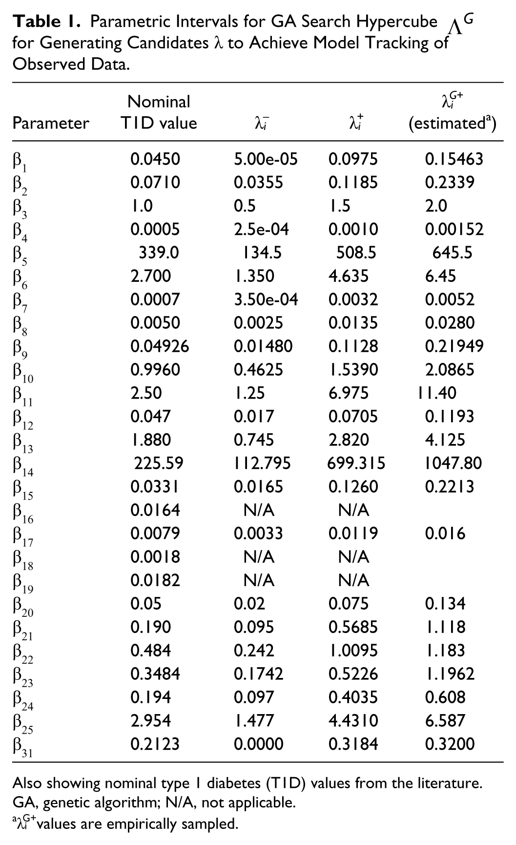
Also showing nominal type 1 diabetes (T1D) values from the literature. GA, genetic algorithm; N/A, not applicable.

a

${\lambda }_i^{G+}$ values are empirically sampled.

• Identification employed a technique outlined by Greenwood. ¹⁵ The PSST typically employs Lyapunov functions to achieve nonlinear MRAC, whereby the dynamics of a complex system (equation 1) are made to converge with the noiseless dynamics ( $\mathbf{w}(t)\equiv \mathbf{0}$ ) of a simpler model (equation 2); the parameters of this simpler model are changed adaptively using a descent condition of one Lyapunov function (typically denoted Vm), while an adaptive controller law is generated using another Lyapunov function (typically denoted $V_S$ ), forcing the system to track the model even under conditions of noise-polluted partial information. Greenwood ¹⁵ indicated that this process can be inverted to enable the identification of complex nonlinear biological systems; provided the model (equation 2) has comparable complexity to the system (equation 1), then the use of historical medication data instead of an adaptive control law forces the descent condition of Vm to reconstruct candidate sets of parameter values and model structures for the underlying system, as the model converges to the system instead of vice versa.

• The previous objections to linearization in the control law also posed an obstacle to formulating an appropriate state observer that would estimate values of unseen variables over time.

• Using the technique outlined above, derived from Greenwood, ¹⁵ enabled the direct construction of multiple underdetermined nonlinear candidate models using all available information. Each candidate generated an associated solution trajectory; the compact set comprising the volume enclosed by all such trajectories (the “dynamic envelope”) bounded the actual system trajectory by exploiting the convergent dynamics of the PSST. Combined with differential game theory, this dynamic envelope replaced the requirement for a single nonlinear observer.

• This alternative technique used a variant of a genetic algorithm (GA). This is a method^28-30 of achieving pattern recognition through simulating the processes of evolution at a chromosomal level. Parameter values from across a compact hypercube were inserted into one or more specified models and evolved across generations through a process of selective breeding and mutation until a pattern of observed data was heuristically matched.

• Candidate vectors $\lambda \in {\Lambda }^{\square }$ , such that the solution trajectories $\phi$ to equation 2 (defined such that $\xi (t)=\phi (\xi (t_0),\lambda ,\mathbf{w}(t),t)|t\in [t_0,t_f]$ ) successfully tracked observed medical data ${\{\mathbf{y}(t_k)\}}_{k=0}^Q$ , were rewarded with enhanced fitness in the selection process, encouraging the evolutionary emergence of parameter sets fitting the model (equation 2) to a known medical history.

This variant of a GA expressed chromosomes using the Gray code ³¹ instead of conventional binary encoding to avoid the formation of Hamming walls. ³⁰ Consequently, the operation of mutation and crossover on the genes of Gray-encoded chromosomes expanded the search domain from an initial compact hypercube $\Lambda$ of plausible values to some larger compact hypercube ${\Lambda }^G,\Lambda \subseteq {\Lambda }^G\subset {ℝ}^m$ , estimated in Table 1.

• In the AP context, this enabled the exploitation of existing T1D models and direct data mining of individual patients’ medical histories to generate multiple, personalized candidates for T1D dynamics consistent with known analytical models and observable data from that individual.

• In contrast with the application of LPV methods to the AP, ¹⁹ here, information about stability of the insulin-based control of the full nonlinear model can be obtained directly using the minimax of the Lyapunov derivatives, where the controller is playing against the known dynamic uncertainties remaining in all plausible candidates ( $\lambda \in {\Lambda }^{\square }$ ).

Information about the level of confidence in imposing stable control (in differential game theory, the “strong controllability”) of the underdetermined system is provided by this method by generating a dynamic envelope of possible solution trajectories and striving to pour this envelope down the slope of the Lyapunov function to the target set (here including a desired interval of BG levels), despite intelligent counterstrategies exploiting known residual uncertainties to attempt to prevent this. Perturbations or uncertainties in the dynamics, if contained within this envelope over time, are then also controlled to target.

This method encompasses not only control of the actual uncertainties across $\lambda \in {\Lambda }^G$ associated with an underdetermined system but also other dynamic uncertainties in the system, such that their effects could be enclosed within a dynamic envelope generated by the model equations using an appropriate choice of some set ${\left\{{\lambda }_j\right\}}_{j=1}^N\subset {\Lambda }^G$ . This was effectively demonstrated in this study by strongly controlling the uncertain effects of meals on the dynamic system.

2. Model Analysis and Manipulation

The key problem was extracting an insulin control law from multiple underdetermined T1D models built from a common high-dimensional set of nonlinear differential equations, which fulfilled desired control objectives using incomplete information.

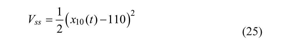
• The solution involved Lyapunov functions. These are typically defined to be positive-definite $C^1$ quadratic functions $V(\mathbf{x}):{ℝ}^n\to {ℝ}_{+}$ , where $V(\mathbf{x})\ge 0$ , $V(\mathbf{x})=0\leftrightarrow \mathbf{x}=\mathbf{0}$ , where $\mathbf{x}={[x_1,\dots ,x_n]}^T\in \Delta \subset {ℝ}^n$ denotes the state of the system being studied, and $\Delta$ is defined to be some biologically relevant subset of state space. $V(\mathbf{x})$ acts as a basin (Figure 1), with the target set $\mathcal{T}\subset \Delta$ of desired states lying at the bottom of the basin: $\mathcal{T}=\{\mathbf{x}\in \Delta |V(\mathbf{x})\le C\},\mathrm{some}C>0$ .

• Model equations (equation 2) operating under a control program or strategy ${\mathbf{u}}_1(t)=\mathbf{p}(\xi (t),t)$ generate solution trajectories $\phi$ , where $\xi (t)=\phi (\xi (t_0),\lambda ,\mathbf{w}(t),t)|t\in [t_0,t_f]$ . Lyapunov-based controls then operate by calculating the control program ${\mathbf{u}}_1(t)=\mathbf{p}(\xi (t),t)$ required to generate trajectories $\phi$ with the desired geometric relationship to the surface of $V(\xi )$ , such that the j descend to the desired target despite ongoing uncertainties, that is, given $\xi (t_0)\notin \mathcal{T}$ :

  $${\mathbf{u}}_1(t)=\mathbf{p}(\xi (t),t)|\frac{\partial V}{\partial t}+\nabla V^T\cdot {\mathbf{f}}_m(\xi (t),\lambda ,\mathbf{p}(\xi (t),t),\mathbf{w}(t),t)\le 0.$$

  (4)

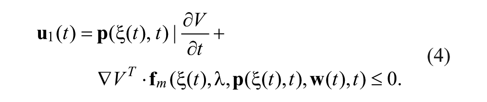
• Equation 4 represents a sufficient condition for stable control of the system. The preferred form of control corresponds with the strongest such form of stability, namely, asymptotic control to target $\mathcal{T}$ . By imposing strict inequality in equation 4, Skowronski ⁷ gives equation 4 as sufficient for asymptotic control if $\mathcal{T}$ is a neighborhood of natural equilibria of the system (equation 1) and further provides a sufficient condition for making a model strongly controllable for asymptotic stability, namely,

$${\mathbf{u}}_1(t)=\mathbf{p}(\xi (t),t)|\frac{\partial V}{\partial t}+\nabla V^T\cdot {\mathbf{f}}_m(\xi (t),\lambda ,\mathbf{p}(\xi (t),t),\mathbf{w}(t),t)\le -c(||\xi (t)||)<0,$$

(5)

where $c:ℝ\to {ℝ}_{+}$ is some continuous positive-definite function for all uncertainties $\mathbf{w}(t)$ , such that $||\mathbf{w}(t)||\le w^{+}<\infty$ .

• Lyapunov-based control is typically formally suboptimal under conditions of perfect information. However, when controlling a complex nonlinear system under conditions of incomplete information and unknown dynamic aspects, the Lyapunov approach has the following advantages:

$${\mathbf{u}}_1|\underset{||\mathbf{w}||\le w^{+}}{\sup }\frac{\partial V}{\partial t}+\nabla V^T\cdot {\mathbf{f}}_m(\xi (t),\lambda ,{\mathbf{u}}_1,\mathbf{w},t)<0$$

(6)

for asymptotically stable controls and

$${\mathbf{u}}_1|\underset{||\mathbf{w}||\le w^{+}}{\sup }\frac{\partial V}{\partial t}+\nabla V^T\cdot {\mathbf{f}}_m(\xi (t),\lambda ,{\mathbf{u}}_1,\mathbf{w},t)\le -c(||\xi (t)||)<0$$

(7)

for strong controllability, ensuring asymptotically stable controls.

Figure 1.

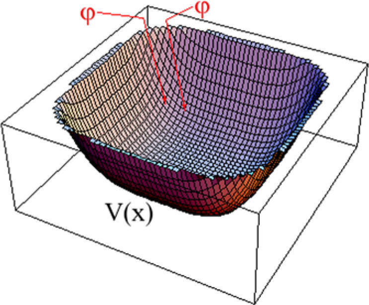
Plot of Lyapunov function showing the descent of solution trajectories towards the target.

This approach was applied to poorly modeled components of the T1D system’s nonlinear dynamics to ensure high-confidence controller stability.

• Estimated regions of controllability are readily computable; such estimates are based on sufficient conditions^6,7 so they are conservative and high confidence.

• Designing a controller law using Lyapunov conditions imposes asymptotic stability on the resulting dynamics within the region of controllability; hence, the strongest available form of stability has been imposed as part of the design process.^6,7

• Real-time computation is fast (an algebraic descent condition); hence, Lyapunov methods have been studied for possible real-time military use.^17,32 This also means that an additional layer of machine-intelligent computation can be introduced to operate within a feasible time, as is done here.

3. Response to Constraints

Significant dynamic constraints affect AP control:

• Changes in ISFG values dynamically lag behind their BG counterparts by a time period that varies based on local BG conditions ³³ and in ways that may not be entirely described by current models.^{34 -36}

• A significant fixed-value CGM sensor lag also exists as an artifact of the ISFG sensors’ filter algorithms.

• CGM has difficulty tracking hypoglycemia directly.^35,37

• Elsewhere, synthetic insulin, once infused subcutaneously, continues to act on BG levels for a considerable duration. The value of this duration of action depends on local dynamic conditions as well as the form of insulin being used.

Consequently, this demonstration did not use CGM data for direct prediction of system dynamics, nor did it assume a specific horizon for a past insulin dose. Both issues were instead resolved through the predictive use of a large number of candidate solution trajectories, generated from the model equations using underdetermined evolutionary fitting to the patients’ available medical histories:

• Partial system identification via data mining medical histories using a variant of a GA gave multiple candidate values for parameters in self-consistent combinations, including those relating ISFG to BG (and similarly for insulin, assuming consistent use of a single insulin type).

• These various values generated multiple trajectories, forming a forward-moving divergent dynamic envelope of the actual system dynamics.

Ongoing CGM data were used to establish recent past values for ISFG and reassess expected recent values for BG, updating the starting point for the dynamic envelope in the recent past every 5 minutes. Thus, CGM data still formed part of a closed-loop AP control but were not used for direct prediction (performed instead by the dynamic envelope). To emphasize the robustness of this approach, in these simulations, the fixed-value CGM sensor lag was taken to be relatively large: ${\tau }_{CGM}=10\mathrm{minutes}.$

4. Modeling of Meals

Meals represent a major source of uncertainty in BG dynamics, with carbohydrate content difficult to predict accurately for most patients with diabetes. Consequently, the AP literature typically imposes strict constraints on meal carbohydrate content, timing, or both^38,39 and views meals as a “disturbance that must be rejected by the control law implemented within the AP algorithm.” ³⁹

This study took a different view: meals are an inherent, if highly uncertain, part of the T1D system dynamics. Their effects are not a disturbance to be rejected but are handled by the control law applying game theory on the dynamic envelope (below).

To demonstrate this, WM3’s medical history provided actual meal data from several months in 2008, which were used in this study:

• Meals were irregularly timed and had irregular carbohydrate content.

• The algorithm received only 10 minutes’ warning before each meal (this constraint was deliberately harsh to emphasize the algorithm’s robustness to short-warning perturbations; in real-world applications, a longer-duration warning would be feasible).

• Estimates of meals’ carbohydrate content were initially assumed accurate, and then robustness studies were performed using ±25% error.

5. Machine-Intelligent Handling of Uncertainty: Game Against Nature

The model dynamics had 2 forms of significant uncertainty:

1. Uncertainties in the values of parameters and state variables due to underdetermined equations, manifested by the dynamic envelope, and

2. Uncertainty associated with an inherently uncertain variable (meal carbohydrates), affecting this dynamic envelope as it flowed through state space.

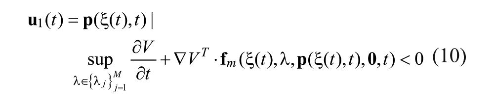
The solution to handling these dynamic uncertainties was to overlay the so-called Game against Nature as an additional layer of machine-intelligent decision making on top of the Lyapunov formulation.^{11,14,16,17,40}

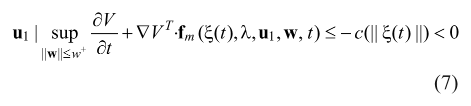
Equation 4 shows the essential criterion for steering a trajectory to a target set despite uncertainty. The Lyapunov-based Game against Nature (L-GaN) goes further, assuming all such (bounded) uncertainty $||\mathbf{w}(t)||\le w^{+}$ is being manipulated intelligently by a hostile player (“Nature”) to thwart these control efforts. The counterstrategy then played is a revised ${\mathbf{u}}_1(t)=\mathbf{p}(\xi (t),t)$ , such that equation 6 is nonetheless obeyed as far as possible.

In the L-GaN implementation demonstrated, the dominant uncertainty was the underdetermined model equations partially identified from available data, leading to a finite set of possible parameter vectors ${\left\{{\lambda }_j\right\}}_{j=1}^N\subset {\Lambda }^G$ , consistent with the observed data for that participant under the T1D model. This generated a finite set of candidate trajectories ${\left\{\phi (\xi (t_0),{\lambda }_j,\mathbf{0},t)|t\in [t_0,t_f]\right\}}_{j=1}^N$ that formed the dynamic envelope. Nature chose which trajectory represented the actual system at any given moment. Equation 6 then implied that the desired requirement was to find

$${\mathbf{u}}_1(t)=\mathbf{p}(\xi (t),t)|\underset{\lambda \in {\left\{{\lambda }_j\right\}}_{j=1}^N}{\sup }\frac{\partial V}{\partial t}+\nabla V^T\cdot {\mathbf{f}}_m(\xi (t),\lambda ,\mathbf{p}(\xi (t),t),\mathbf{0},t)<0,$$

(8)

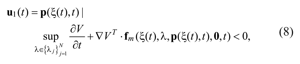
with the preferred form (from equation 7)

$${\mathbf{u}}_1(t)=\mathbf{p}(\xi (t),t)|\underset{\lambda \in {\left\{{\lambda }_j\right\}}_{j=1}^N}{\sup }\frac{\partial V}{\partial t}+\nabla V^T\cdot {\mathbf{f}}_m(\xi (t),\lambda ,\mathbf{p}(\xi (t),t),\mathbf{0},t)\le -c(||\xi (t)||)<0.$$

(9)

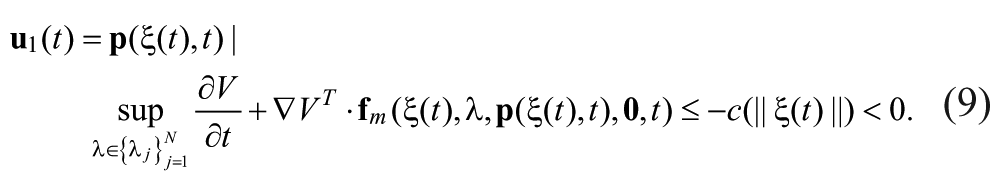
When no single strategy satisfied equations 8 or 9 for all $\lambda \in {\left\{{\lambda }_j\right\}}_{j=1}^N$ at a particular state $\xi (t)$ , a form of “triage logic” was applied by the algorithm to find ${\mathbf{u}}_1(t)=\mathbf{p}(\xi (t),t)$ , satisfying

$${\mathbf{u}}_1(t)=\mathbf{p}(\xi (t),t)|\underset{\lambda \in {\left\{{\lambda }_j\right\}}_{j=1}^M}{\sup }\frac{\partial V}{\partial t}+\nabla V^T\cdot {\mathbf{f}}_m(\xi (t),\lambda ,\mathbf{p}(\xi (t),t),\mathbf{0},t)<0$$

(10)

for some ${\left\{{\lambda }_j\right\}}_{j=1}^M\subset {\left\{{\lambda }_j\right\}}_{j=1}^N,$ with the condition that $\mathbf{p}(\xi (t),t)$ and $M$ were chosen to satisfy the following preference ordering:

1. If possible, all candidate parameter vectors associated with trajectories projecting hypoglycemia from $\xi (t)$ were to be included in $\lambda \in {\left\{{\lambda }_j\right\}}_{j=1}^M$ .

2. If not all ${\lambda }_j$ projecting hypoglycemia could be included under a single strategy $\mathbf{p}(\xi (t),t)$ , then $\mathbf{p}(\xi (t),t)$ was chosen to include the most significant such ${\lambda }_j$ (i.e, those projecting the most dangerous hypoglycemic episodes).

3. Subordinate to the above, $\mathbf{p}(\xi (t),t)$ was chosen to include in ${\left\{{\lambda }_j\right\}}_{j=1}^M$ the maximal number of ${\lambda }_j$ (if any), projecting hyperglycemia from $\xi (t)$ .

4. Subordinate to the above, $\mathbf{p}(\xi (t),t)$ was then chosen for maximal $M$ .

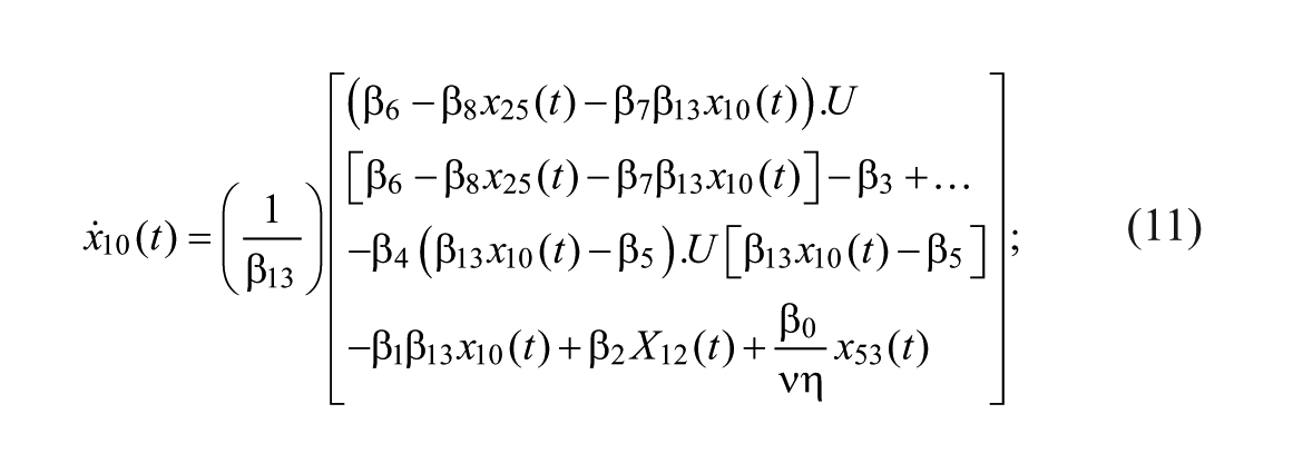
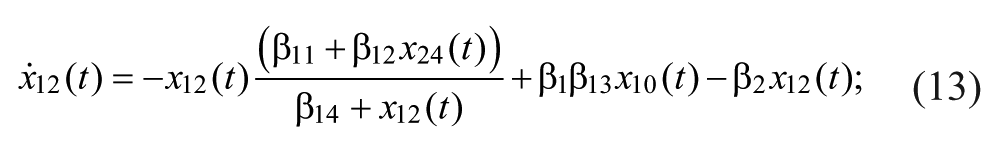
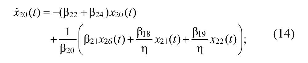
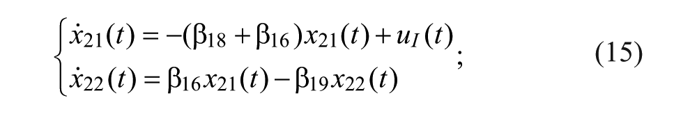
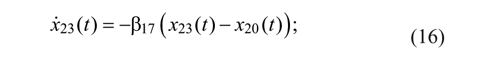
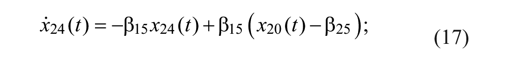
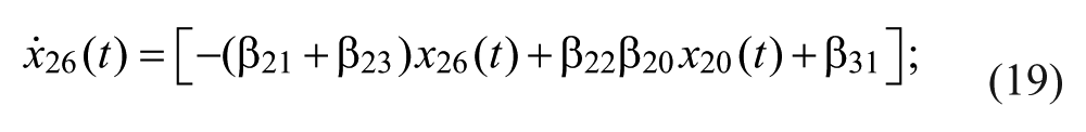
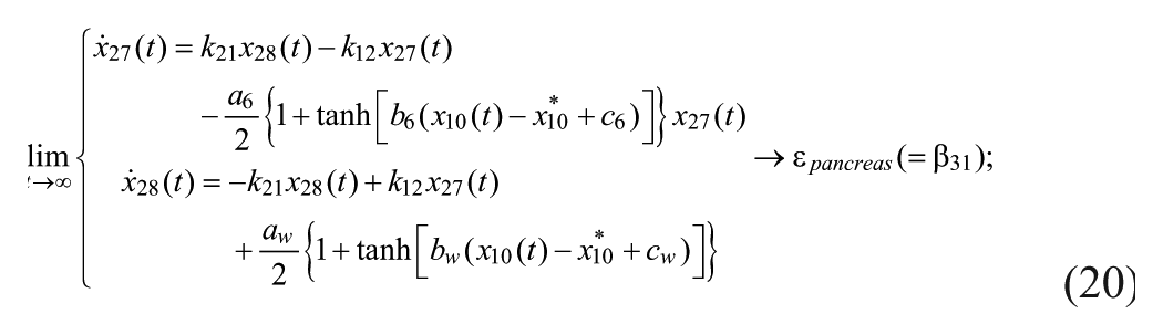
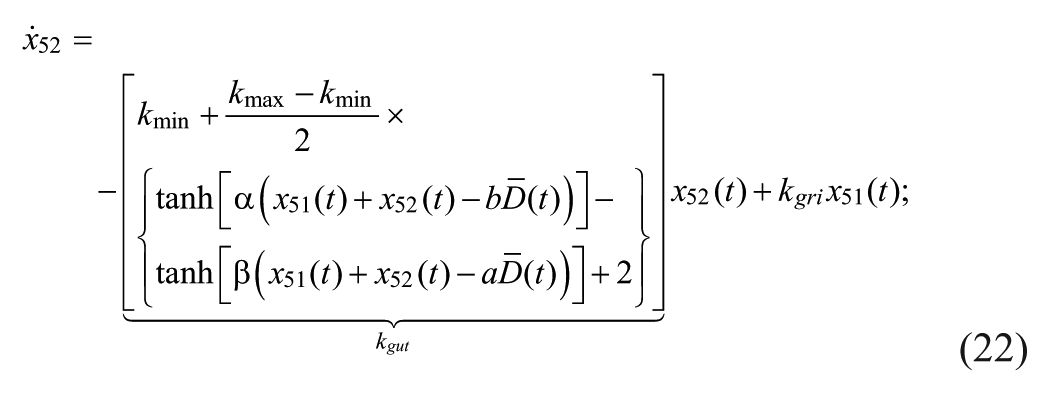
The T1D system was primarily derived from Magni et al ²² with four modifications:

1. The unit step function $U[z]\triangleq \{\begin{array}{c}1,z\ge 0\\ 0,z<0\end{array}$ was introduced to handle on/off switching of the renal excretion of glucose and endogenous glucose production.

2. A dimensional anomaly was found in the BG-ISFG dynamics of Magni et al. ²² This was remedied by inserting an additional term corresponding with $g\in [0.925,1.026]$ from Facchinetti et al. ³³

3. Meal equations were taken from Magni et al ²² and Dalla Man et al. ⁴¹ The medical histories of “brittle” patients with diabetes at Westmead Hospital demonstrated significantly higher glycemic sensitivity than predicted by Dalla Man et al, ⁴¹ so a correction factor $\nu \in (0,1]$ modified the body mass $\eta$ in equation 11 to align the scale of these fluctuations.

4. Clinical T1D typically has vestigial pancreatic insulin secretion, complicating insulin control. To simulate the presence of this tiny insulin signal, ${\epsilon }_{pancreas}(={\beta }_{31})$ ^25,42 was used via equation 20 for a steady-state approximation.

Then, the system equations were as follows (with variables as defined in Table 2):

Table 2.

Variables in the State Vector $\mathbf{x}(t)$ .

Variable	Meaning
$x_{10}$	Blood glucose concentration (mg/dL)
$x_{11}$	Interstitial fluid glucose concentration (mg/dL)
$x_{12}$	Glucose mass in slowly equilibrating tissue (mg/kg)
$x_{20}$	Insulin concentration in plasma (pmol/L)
$x_{21}$	Nonmonomeric insulin in subcutaneous space (pmol)
$x_{22}$	Monomeric insulin in subcutaneous space (pmol)
$x_{23}$	Insulin variable (pmol/L)
$x_{24}$	Remote insulin signal (pmol/L)
$x_{25}$>	Delayed insulin signal (pmol/L)
$x_{26}$	Liver insulin (pmol/kg)
$x_{27},x_{28}$	Variables relating to vestigial pancreatic insulin synthesis and secretion
$x_{51},x_{52}$	Glucose in solid- and liquid-phase food in stomach (mg)
$x_{26}$	Glucose mass in intestine (mg)
$u_I(t)$	Infused insulin control variable (pmol/kg/min)

$$\begin{array}{l}{\stackrel{.}{x}}_{10}(t)=\left(\frac{1}{{\beta }_{13}}\right)\left[\begin{array}{l}\left({\beta }_6-{\beta }_8{x}_{25}(t)-{\beta }_7{\beta }_{13}{x}_{10}(t)\right).U\\ \left[{\beta }_6-{\beta }_8{x}_{25}(t)-{\beta }_7{\beta }_{13}{x}_{10}(t)\right]-{\beta }_3+\dots \\ -{\beta }_4\left({\beta }_{13}{x}_{10}(t)-{\beta }_5\right).U\left[{\beta }_{13}{x}_{10}(t)-{\beta }_5\right]\\ -{\beta }_1{\beta }_{13}{x}_{10}(t)+{\beta }_2{X}_{12}(t)+\frac{{\beta }_0}{\mathrm{\nu \eta }}{x}_{53}(t)\end{array}\right];\end{array}$$

(11)

$${\stackrel{.}{x}}_{11}(t)=-{\beta }_9{x}_{11}(t)+{\beta }_9{\beta }_{10}{x}_{10}(t);$$

(12)

$${\stackrel{.}{x}}_{12}(t)=-x_{12}(t)\frac{\left({\beta }_{11}+{\beta }_{12}{x}_{24}(t)\right)}{{\beta }_{14}+x_{12}(t)}+{\beta }_1{\beta }_{13}{x}_{10}(t)-{\beta }_2{x}_{12}(t);$$

(13)

$${\stackrel{.}{x}}_{20}(t)=-({\beta }_{22}+{\beta }_{24})x_{20}(t)+\frac{1}{{\beta }_{20}}\left({\beta }_{21}{x}_{26}(t)+\frac{{\beta }_{18}}{\eta }{x}_{21}(t)+\frac{{\beta }_{19}}{\eta }{x}_{22}(t)\right);$$

(14)

$$\{\begin{array}{l}{\stackrel{.}{x}}_{21}(t)=-({\beta }_{18}+{\beta }_{16})x_{21}(t)+u_I(t)\\ {\stackrel{.}{x}}_{22}(t)={\beta }_{16}{x}_{21}(t)-{\beta }_{19}{x}_{22}(t)\end{array};$$

(15)

$${\stackrel{.}{x}}_{23}(t)=-{\beta }_{17}\left(x_{23}(t)-x_{20}(t)\right);$$

(16)

$${\stackrel{.}{x}}_{24}(t)=-{\beta }_{15}{x}_{24}(t)+{\beta }_{15}\left(x_{20}(t)-{\beta }_{25}\right);$$

(17)

$${\stackrel{.}{x}}_{25}(t)=-{\beta }_{17}(x_{25}(t)-x_{23}(t));$$

(18)

$${\stackrel{.}{x}}_{26}(t)=\left[-({\beta }_{21}+{\beta }_{23})x_{26}(t)+{\beta }_{22}{\beta }_{20}{x}_{20}(t)+{\beta }_{31}\right];$$

(19)

$$\underset{t\to \infty }{\lim }\{\begin{array}{c}{\stackrel{.}{x}}_{27}(t)=k_{21}{x}_{28}(t)-k_{12}{x}_{27}(t)-\frac{a_6}{2}\left\{1+\tanh \left[b_6(x_{10}(t)-x_{10}^{*}+c_6)\right]\right\}{x}_{27}(t)\\ {\stackrel{.}{x}}_{28}(t)=-k_{21}{x}_{28}(t)+k_{12}{x}_{27}(t)+\frac{a_w}{2}\left\{1+\tanh \left[b_w(x_{10}(t)-x_{10}^{*}+c_w)\right]\right\}\end{array}\to {\epsilon }_{pancreas}(={\beta }_{31});$$

(20)

$${\stackrel{.}{x}}_{51}=-k_{gri}{x}_{51}+d(t);$$

(21)

$$\begin{array}{l}{\stackrel{.}{x}}_{52}=\\ -\underset{k_{gut}}{\underbrace{\left[\begin{array}{l}{k}_{\min }+\frac{k_{\max }-k_{\min }}{2}\times \\ \left\{\begin{array}{l}\tanh \left[\alpha \left(x_{51}(t)+x_{52}(t)-b\overline{D}(t)\right)\right]-\\ \tanh \left[\beta \left(x_{51}(t)+x_{52}(t)-a\overline{D}(t)\right)\right]+2\end{array}\right\}\end{array}\right]}}{x}_{52}(t)+k_{gri}{x}_{51}(t);\end{array}$$

(22)

$${\stackrel{.}{x}}_{53}=-\frac{{\beta }_0}{f}{x}_{53}(t)+k_{gut}{x}_{52}(t).$$

(23)

The components of $\beta$ were system parameters to be partially identified (except ${\beta }_{16},{\beta }_{18},{\beta }_{19}$ ; see below); all other system parameters use symbols defined in relevant works.^{21,22,25,41,42}

• For each participant, $\beta$ was permanently hidden within a “black box,” as were nonmeal components of the state vector $\mathbf{x}(t)$ , partly revealed by measurements of BG $\left({\{y_{10}(t_k)\}}_{k=0}^{Q_{BG}},y_{10}(t_k)\equiv x_{10}(t_k)\right)$ , ISFG $\left({\{y_{11}(t_k)\}}_{k=0}^{Q_{ISFG}},y_{11}(t_k)\equiv x_{11}(t_k)\right)$ , and sometimes PI $\left({\{y_{20}(t_k)\}}_{k=0}^{Q_{PI}},y_{20}(t_k)\equiv x_{20}(t_k)\right)$ .

• Partial identification was to be achieved through generation of vectors $\lambda$ and associated model state vectors $\xi (t)$ that predicted the observed measurements.

• Apart from ${\beta }_0$ , meal equations 21 to 23 were not to be identified, as the major uncertainties—meal carbohydrate content, candidate values of ${\lambda }_0$ , and other parameters in ${\stackrel{.}{\xi }}_{10}(t)$ —dominated other meal-related dynamics.

A related question in this study was the impact on stable insulin control of PI assay (non)availability during identification:

• PK parameters for subcutaneous insulin infusion were assumed to be well estimated by the insulin manufacturer and available to the clinician. Reassessing existing manufacturers’ estimates of insulin infusion PK using these algorithms is possible but was regarded as a less interesting question than exploring the deeper capabilities of these algorithms in tandem with existing estimates, with and/or without PI time series being available, so accurate infusion PK estimates were assumed.

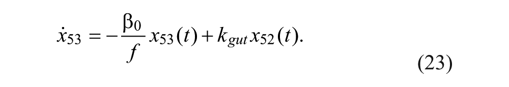
  Consequently, equation 15 was replaced by equation 24:

  $$\{\begin{array}{l}{\stackrel{.}{x}}_{21}(t)=-(k_{a_1}+k_d)x_{21}(t)+u_I(t)\\ {\stackrel{.}{x}}_{22}(t)=k_d{x}_{21}(t)-k_{a_2}{x}_{22}(t)\end{array}.$$

  (24)

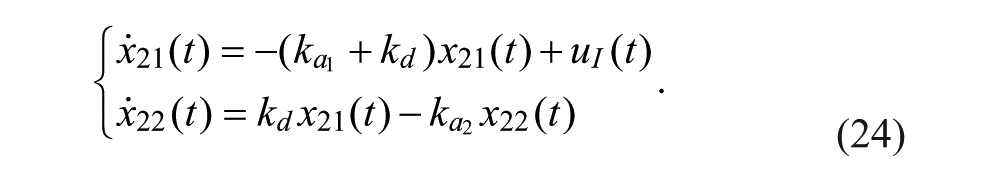
• Were this assumption to be abandoned, the same identification techniques demonstrated here would be repeated for ${\beta }_{16},$ ${\beta }_{18},$ , and ${\beta }_{19},$ ; however, this would then necessitate a PI time series.

The literature^{21,22,24,25,33,41 -44} gave possible ${\beta }_i$ values, whereby variation among patients with diabetes and healthy participants typically produced a maximal interval $[{\beta }_i^{-},{\beta }_i^{+}].$

• When such intervals existed, an associated search interval $[{\lambda }_i^{-},{\lambda }_i^{+}]=[0.5{\beta }_i^{-},1.5{\beta }_i^{+}]$ was constructed for the identifier using a further ±50% tolerance to emphasize method robustness. When only a single value ${\beta }_i^{°}$ was published, this interval became $[{\lambda }_i^{-},{\lambda }_i^{+}]=[0.5{\beta }_i^{°},1.5{\beta }_i^{°}]$ .

• The parametric plausible candidate hypercube $\Lambda =[{\lambda }_0^{-},{\lambda }_0^{+}]\times \dots \times [{\lambda }_{31}^{-},{\lambda }_{31}^{+}]$ was then constructed (without intervals for ${\beta }_{16},{\beta }_{18},{\beta }_{19}$ , ${\beta }_{26}\mathrm{to}{\beta }_{30}$ ). Recombination and mutation on Gray-encoded genes caused the effective upper bounds of these gene intervals to expand, forming a larger parametric search hypercube ${\Lambda }^G=[{\lambda }_0^{-},{\lambda }_0^{G+}]\times \dots \times [{\lambda }_{31}^{-},{\lambda }_{31}^{G+}]$ (Table 1).

Hence, using the standard “black box” method for simulation testing, vectors of system parameters ${\beta }_{S1}$ and ${\beta }_{S2}$ were constructed for 2 patients with diabetes, S1 and S2, and hidden from both the identifier and controller in a “black box” participant simulator:

• S1 used representative T1D values from the above literature, as a “typical” patient with diabetes (basal BG = 179.5 mg/dL).

• S2 was modified within the plausible range of diabetic values to reflect more extreme behavior observed in a “brittle” patient with diabetes (in particular, basal BG = 231.7 mg/dL), chosen to be challenging to reduce the desired BG interval [80, 140] mg/dL without either inducing hypoglycemia or experiencing interim hyperglycemia.

Using 61 days’ actual meal and insulin pump data from WM3’s medical history, ${\beta }_{S1}$ and ${\beta }_{S2}$ were used by the “black box” to generate by simulation nineteen 24-hour days of complete medical histories (using equivalent dates: September 23, 2008; July 25 to August 11, 2008) for these 2 participants, assuming fingerstick measurements every 2 hours and CGM measurements every 5 minutes.

The observable time series from these medical histories were given to the identifier to analyze. Identification involved hypothesis formulation and predictive testing on independent data. Up to 11 days’ actual meal data were also used for the controller phase. Throughout identification, the “tracking criterion” was that trajectories must track fasting BG and ISFG measurements to within ±1 mg/dL and PI data, where measured, within ±5 pM.

Results

Computational processes were divided between time-intensive identification, performed offline prior to the controller regime, and the controller, which was demonstrated to operate effectively in real time (computations required in 10 minutes’ simulated time were performed within 10 minutes in real time).

For each participant, the process was as follows.

Stage 1: Initial Identification

This was performed on a single day’s fasting data (September 23) 7.5 hours from midnight to breakfast.

For each participant, two scenarios were studied:

1. (I): PI assays accompanied each fasting BG measurement in stage 1, and

2. (No I): no such PI measurements were available.

Running in a parallel-computing architecture using an AMAX Servmax MNL-1185 (AMAX, Fremont, California) high-performance server, equipped with 2 quad-core Intel Xeon E5520 (Intel, Santa Clara, California) Nehalem processors and 3 Nvidia Tesla C1060 (Nvidia, Santa Clara, California) cards, each time, the identifier used 100 chromosomes, initially generated randomly across $\Lambda$ in a GA running 10,000 to 15,000 generations to seek vectors ${\left\{{\lambda }_j\right\}}_{j=1}^{100}\subset {\Lambda }^G$ that complied with (ie, tracked within criterion) the observed time series measurements of the “black box” system when responding to insulin infusion.

This was done using 10 to 15 runs per participant per scenario, generating an analysis of 10 million to 22.5 million (typically 15 million) candidate vectors each. Table 3 lists the numbers of compliant vectors/candidate trajectories derived from fasting data, each corresponding with an initial hypothesis of the system dynamics based on incomplete information. Note that the severely underdetermined nature of the identification process and the nonlinearity and complexity of system and model equations meant that the possibility of large-scale divergent dynamics remained: models constructed on ${\Lambda }^G$ would not necessarily track the system dynamics, emphasized by Table 3, which typically extracted fewer than 1600 acceptable hypotheses out of millions of chromosomes.

Table 3.

Number of Hypotheses per Participant and Scenario.

Participant (PI scenario)	Number of Stage 1–compliant hypotheses	Number of final hypotheses in reduced dynamic envelope
S1 (I)	1106	549
S1 (No I)	1571	535
S2 (I)	1017	621
S2 (No I)	1115	894

(I), scenario where plasma insulin (PI) assays are available in Stage 1 identification; (No I), scenario where PI assays are unavailable.

Stage 2: First-Pass Fasting Open-Loop Predictive Testing

• Using 8 distinct days’ fasting insulin infusion data (6-8 hours daily; July 25 to August 1), hypotheses predicted BG and ISFG trajectories each day, which were compared with “black box” measurements. All compliant stage 1 hypotheses tracked the measurements each day within the tracking criterion.

• This was then successfully repeated using another 10 days’ fasting data (6-8 hours daily; August 2-11).

Stage 3: First-Pass Open-Loop Prandial Filter

Insulin infusion and meal time series across September 23 were then supplied to the hypotheses, which predicted BG and ISFG time series for 24 hours.

• Given the uncertainty associated with meal dynamics, the key question was whether the dynamic envelope encompassed all known system behavior.

• The dynamic envelope was indeed observed to surround all actual “black box” postprandial BG and ISFG measurements (Table 4, left-hand column: BG data shown as squares).

• As the hypotheses were generated under fasting conditions, some trajectories diverged significantly from observed postprandial BG behavior while still imposing an envelope upon it. Those diverging too far from observed BG levels were culled as extraneous to reflect the observed meal dynamics reality and reduce the computational burden of the L-GaN. Table 3 shows the number of remaining hypotheses in the “reduced” dynamic envelope, illustrated in Table 4 (left-hand column) for both participants and both scenarios, including the associated tracking/prediction of PI time series (right-hand column). Note that the actual PI time series (dashed blue line) had its waveform successfully predicted as a candidate, when PI data were unavailable.

Table 4.

Construction of the Reduced Dynamic Envelope.

S1 (I) (September 23)
S1 (No I) (September 23)
S2 (I) (September 23)
S2 (No I) (September 23)

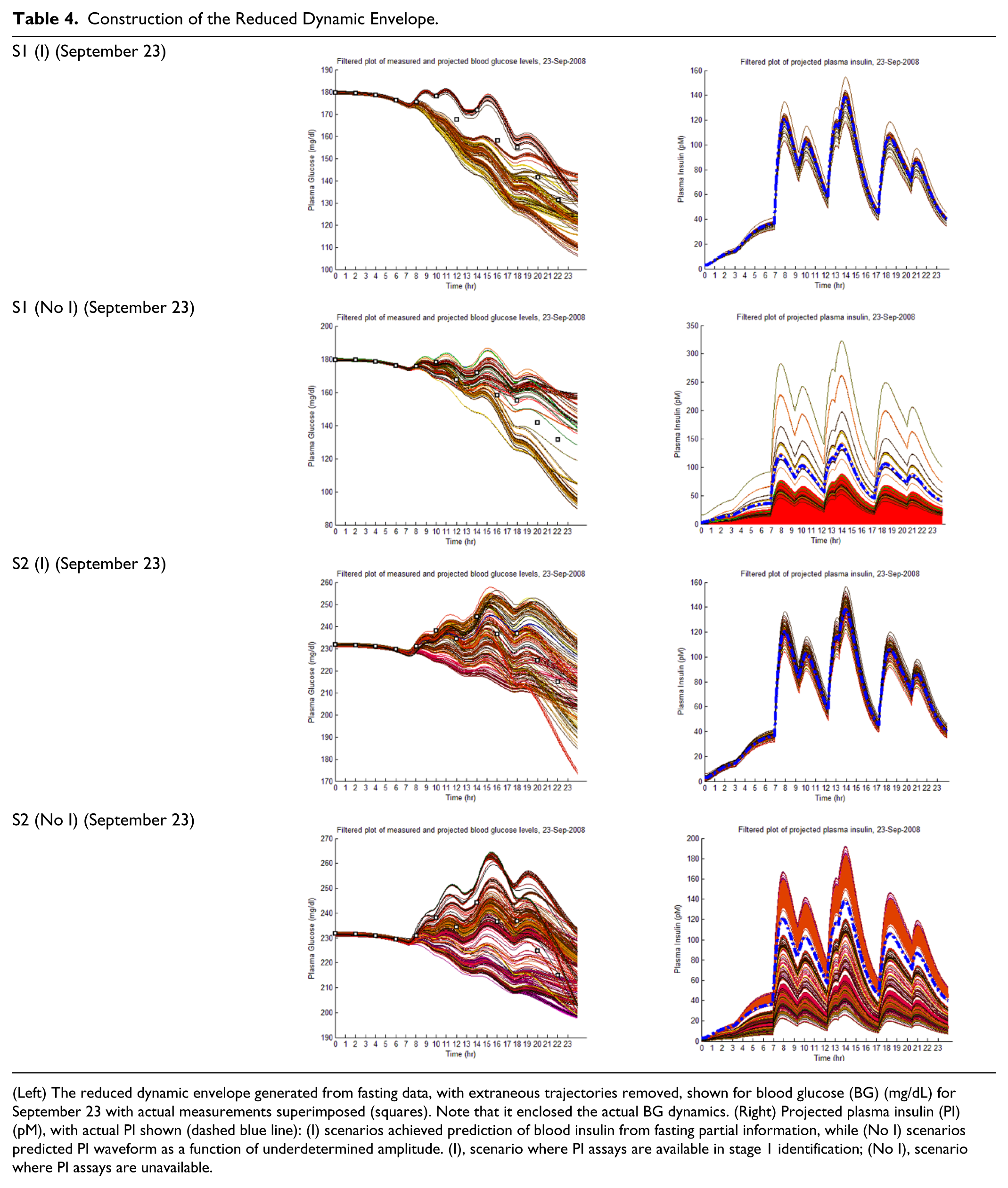
(Left) The reduced dynamic envelope generated from fasting data, with extraneous trajectories removed, shown for blood glucose (BG) (mg/dL) for September 23 with actual measurements superimposed (squares). Note that it enclosed the actual BG dynamics. (Right) Projected plasma insulin (PI) (pM), with actual PI shown (dashed blue line): (I) scenarios achieved prediction of blood insulin from fasting partial information, while (No I) scenarios predicted PI waveform as a function of underdetermined amplitude. (I), scenario where PI assays are available in stage 1 identification; (No I), scenario where PI assays are unavailable.

Stage 4: Second-Pass Open-Loop Prandial Predictive Testing

• Remaining hypotheses were given whole-of-day meal and insulin infusion time series for 10 distinct days (August 2-11) and generated predictions for BG and ISFG, which were then compared with “black box” measurements for consistency.

• The dynamic envelopes passed all the stages of testing and thus were deemed suitably robust as a predictive tool.

The next part of the study was to demonstrate the L-GaN closed-loop controller applying the triage logic of equations 8 and 10 to the participants under both scenarios. On each of 5 to 11 days (September 23 repeated as a common benchmark; additional days from August 2-11), the closed-loop controller was tasked with steering BG levels to the desired target ${\mathcal{T}}_{BG}=[80,140]\mathrm{mg}/\mathrm{dl}$ via insulin infusion, using the relevant dynamic envelope while avoiding hypoglycemia (<70 mg/dL) or high BG/hyperglycemia (>160 mg/dL). Meal time series were communicated to the controller as specified in the Methods section.

The baseline controller sampled BG every 2 hours and ISFG using the ongoing flow of CGM data every 5 minutes and assumed accurate carbohydrate estimates. Control began at 0001 hours each day, with the controller recomputing strategies on a time scale of minutes. To emphasize algorithm stability, each day was treated in isolation, beginning at basal conditions (instead of successor days benefitting from previous successful BG control).

To distinguish between initial high BG conditions and subsequent hyperglycemia, a grace period of 6 hours (midnight to 0600 hours) was permitted when logging nonhypoglycemic BG levels to handle the daily descent from basal conditions (Figure 2). Hypoglycemic events (if any) were to be recorded over the full 24 hours.

Figure 2.

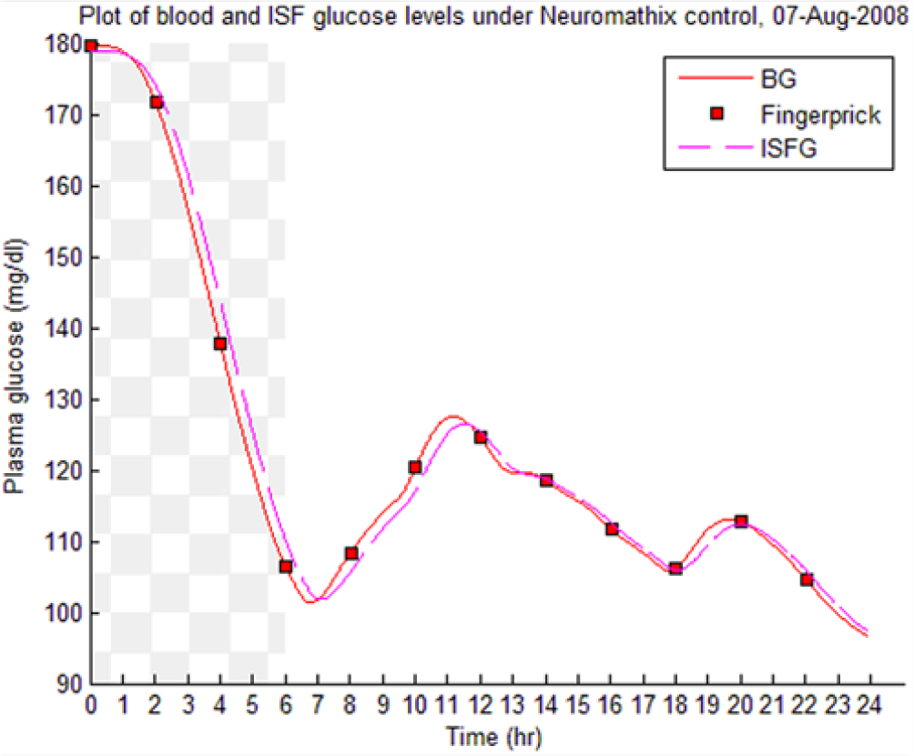
Plot of successful Lyapunov-based Game against Nature control of blood glucose, showing controlled descent during the “grace period” (checkered) and controlled meal perturbations.

As shown in Tables 5 and 6, the baseline L-GaN insulin control was successfully established, with no high BG occurring after 0600 hours, or hypoglycemia at any time, over 38 simulated days. In the case of S2, BG fingerstick samples were then relaxed to every 4 hours to assess this effect on performance over 5 additional simulated days.

Table 5.

Results of Baseline L-GaN Control for S1.

BG level, mg/dL	Status	WM3: CGM data (actual insulin; September 23), %	S1: reference (WM3 insulin; September 23), %	S1 (I) (September 23 + 10 days), %	S1 (No I) (September 23 + 10 days), %
160+	Hyperglycemia and near hyperglycemia	90.3	65.4
140-160	High intermediate	9.7	20.6
120-140	Desired prandial		14.0	24.2	42.5
80-120	Desired basal and prandial			75.8	57.5
70-80	Low intermediate
0-70	Hypoglycemia

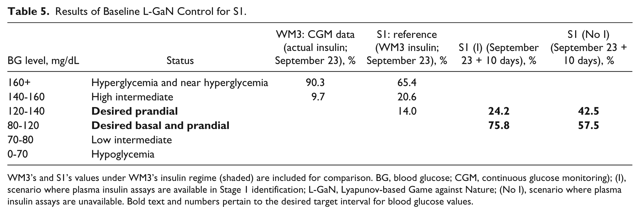
WM3’s and S1’s values under WM3’s insulin regime (shaded) are included for comparison. BG, blood glucose; CGM, continuous glucose monitoring); I, scenario where plasma insulin assays are available in Stage 1 identification; L-GaN, Lyapunov-based Game against Nature; (No I), scenario where plasma insulin assays are unavailable. Bold text and numbers pertain to the desired target interval for blood glucose values.

Table 6.

Results of L-GaN Control for S2: BG Sampling Period of 2 Hours or 4 Hours.

BG level, mg/dL	Status	S2: reference (WM3 insulin; September 23), %	S2 (I) (September 23 + 10 days), %	S2 (No I) (September 23 + 4 days), %	S2 (No I): BG every 4 hours (September 23 + 4 days), %
160+	Hyperglycemia and near hyperglycemia	100.0
140-160	High intermediate		0.5	0.5	0.5
120-140	Desired prandial		9.3	7.9	34.0
80-120	Desired basal and prandial		90.3	91.7	65.5
70-80	Low intermediate
0-70	Hypoglycemia

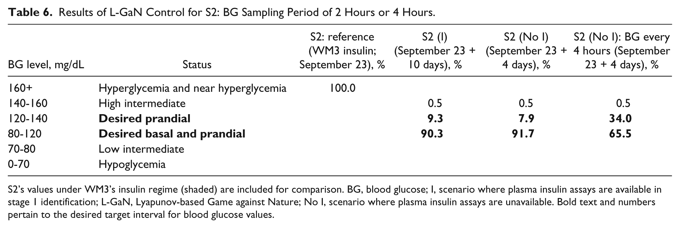
S2’s values under WM3’s insulin regime (shaded) are included for comparison. BG, blood glucose; (I), scenario where plasma insulin assays are available in stage 1 identification; L-GaN, Lyapunov-based Game against Nature; (No I), scenario where plasma insulin assays are unavailable. Bold text and numbers pertain to the desired target interval for blood glucose values.

Meal robustness tests were then performed over 6 days per participant under No I conditions:

• Fingerstick tests were relaxed to every 4 hours.

• In accordance with Patek et al, ³⁹ carbohydrate data communicated to the controller were falsified by ±25% to test robustness to meal uncertainty. To avoid random errors partially canceling, 2 distinct scenarios of daylong systematic errors were tested: systematic +25% and −25% meal errors were applied to all meals across simulation days.

• The +25% test (increasing actual carbohydrate content by 25% over the values given the AP; all meals) used a single day (September 23). The −25% test (reducing actual carbohydrate content by 25% below the values given the AP; all meals) was regarded as more important due to the risk of hypoglycemia from excessive insulin, so it used 5 days’ meal data (September 23, August 2-5) to assess.

Successful, stable closed-loop control was achieved on all days (Table 7), despite this additional uncertainty.

Table 7.

Meal Robustness Tests for L-GaN Control: BG Sampling Every 4 Hours.

BG level, mg/dL	Status	S1 (No I): carbohydrate +25% (September 23), %	S1 (No I): carbohydrate −25% (September 23 + 4 days), %	S2 (No I): carbohydrate +25% (September 23), %	S2 (No I): carbohydrate −25% (September 23 + 4 days), %
160+	Hyperglycemia and near hyperglycemia
140-160	High intermediate	57.3	2.9	0.5	0.5
120-140	Desired prandial	16.9	36.2	67.6	7.4
80-120	Desired basal and prandial	25.7	60.9	31.9	92.1
70-80	Low intermediate
0-70	Hypoglycemia

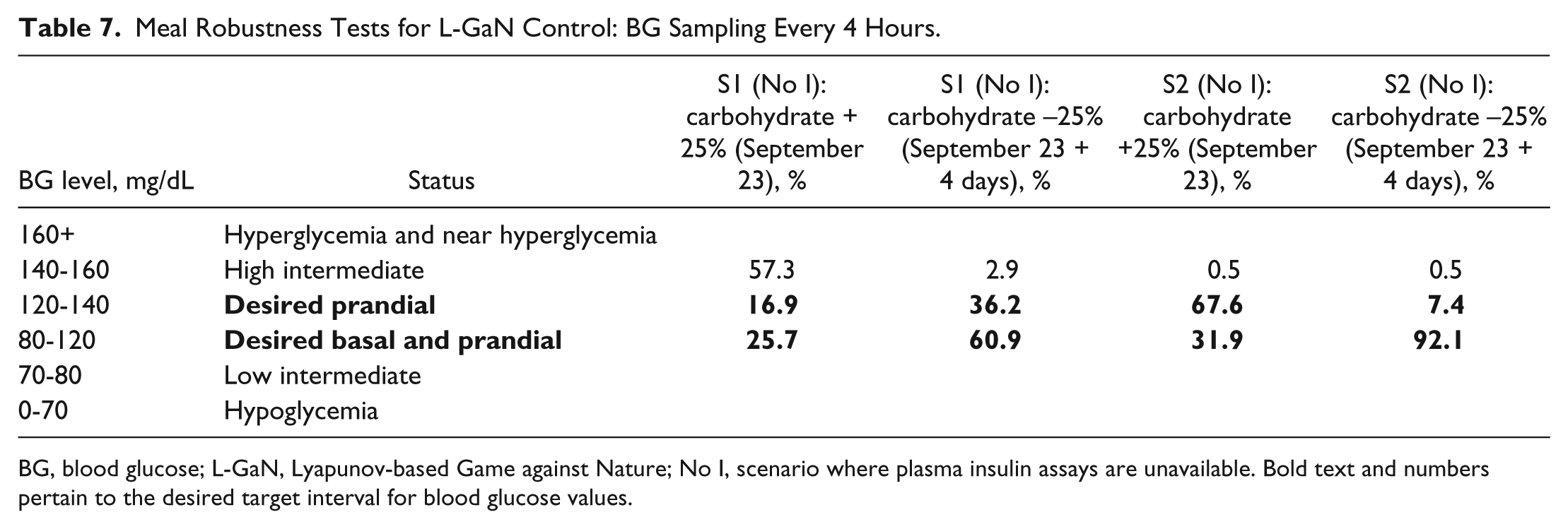
BG, blood glucose; L-GaN, Lyapunov-based Game against Nature; (No I), scenario where plasma insulin assays are unavailable. Bold text and numbers pertain to the desired target interval for blood glucose values.

Hence, stable closed-loop insulin control was successfully demonstrated under realistic meal conditions for both participants under both scenarios, without hypoglycemia or postprandial hyperglycemia, for a total of 55 days.

Discussion

The simulations showed the following:

• Available fasting PI data during identification significantly improved BG control for S1 (Table 5), although it had negligible effects in the analogous S2 baseline study, where the reduced dynamic envelope appeared to be sufficient (Table 6).

• Relaxing fingerstick intervals in the S2 (No I) study to 4 hours had a significant effect on BG levels, shifting BG activity upwards (Table 6).

• As shown in Table 7, the carbohydrate +25% study for S1 pushed BG out of target 57.3% of the time, although no postprandial high BG levels or hyperglycemia ensued. The uncertainty had a negligible effect in the equivalent study for S2, suggesting that S2’s dynamic envelope (profuse ${\lambda }_0$ candidates) was robust against it.

• The reduced dynamic envelopes for both participants were robust against hypoglycemia under the carbohydrate −25% studies in BG levels dropping low gave the antihypoglycemia strategies priority within S1’s dynamic envelope, pushing the subsequent profiles up.

• Table 8 illustrates examples of the stable control for both participants, first under the I scenario with accurate meal data and then under the No I carbohydrate −25% scenario, all using WM3’s actual meal history of August 2 (left-hand column) and August 3 (right-hand column).

• The absence of any hypoglycemic or postprandial high BG levels is attributed to the controller’s application of triage logic to the reduced dynamic envelope generated by the evolutionary identifier.

Table 8.

Examples of BG Plots (mg/dL): August 2 and 3.

S1 (I) (August 2-3)
S1 (No I): carbohydrate −25% (August 2-3)
S2 (I) (August 2-4)
S2 (No I): carbohydrate −25% (August 2-3)

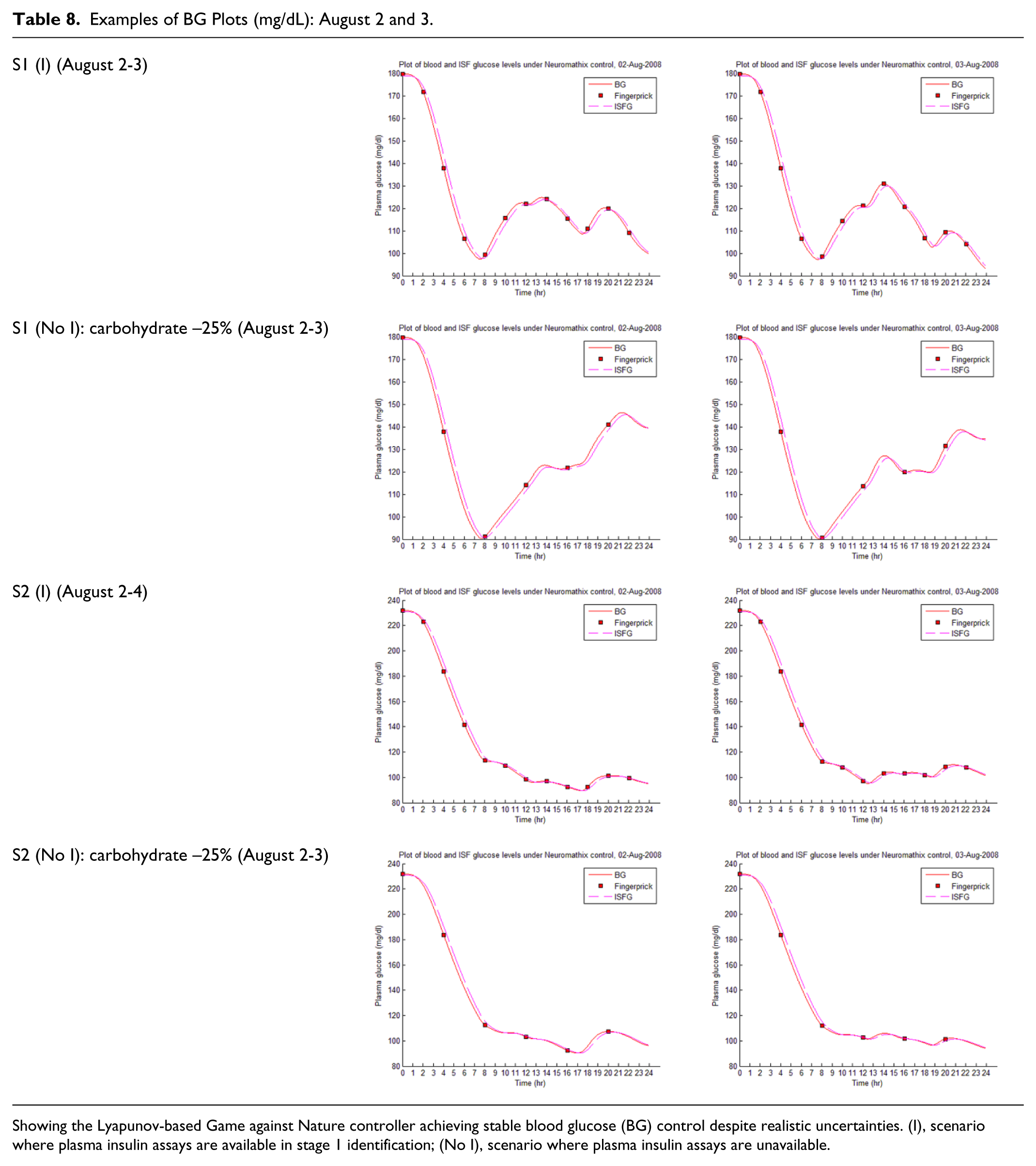
Showing the Lyapunov-based Game against Nature controller achieving stable blood glucose (BG) control despite realistic uncertainties. (I), scenario where plasma insulin assays are available in stage 1 identification; (No I), scenario where plasma insulin assays are unavailable.

A key question for any AP controller for real-world medical deployment is its stability under dynamic perturbations. An advantage of the present technique was that the stability of its Lyapunov controller could be directly analyzed.

Although the controller function $V_S$ was too complicated for easy interpretation, the system dynamics and AP objectives allowed a much simpler function $V_{ss}$ to be used for stability analysis of the controller on BG levels outside the target set $x_{10}(t)\in {\mathcal{T}}_{BG}=[80,140]\mathrm{mg/dl}$ . The dynamics of the system (equation 1) and model (equation 2) were bounded on all variables and inputs and dissipative, with an equilibrium under “basal” conditions. Consequently, the simple positive-definite function

$$V_{ss}=\frac{1}{2}{\left(x_{10}(t)-110\right)}^2$$

(25)

was adequate to test BG stability with respect to the objective of steering the trajectory to the target and retaining it there. Segments of the trajectory within the target T BG were ignored as the objective was already met; however, meal- and insulin-based perturbations enabled the ongoing possibility of target escape or excursions.

Analysis over the 55 days revealed that the controller established strong controllability for asymptotically stable control, the strongest possible form of stable control, as stipulated in equation 7 by 0100 hours every morning, retaining it while steering the trajectory to the target under fasting conditions in preparation for meal-based perturbations that might break stability. Including the daily descent phase from midnight, trajectories were external to the target 21.67% of the overall simulation time. They were under stable control for 99.43% of this period and so suffered formal instability for less than 1% of their overall time external to the target. As shows, the scenario that suffered the most meal-induced breaks in formal Lyapunov stability was the S1 (No I) carbohydrate +25% scenario, where deliberately inputting false meal data caused formal stability to lapse for 19.01% of the 24-hour day, but under this scenario, the algorithm still imposed effective control, preventing all BG excursions from leaving the interval [80, 160] mg/dL.

Conclusions

The key problems confronting stable, high-confidence AP control of BG via insulin infusion are the following:

• Realistic T1D models in the literature are significantly underdetermined when using available time series data.

• Three dynamic uncertainties dominate closed-loop control: namely, BG-ISFG lag, duration of insulin effect, and meal carbohydrate uncertainty.

• Stability of the BG controller algorithm is essential in an uncertain environment.

This study demonstrated that these problems could be solved by resolving them simultaneously: evolving multiple candidate models for a realistic T1D model from partial information and then combining Lyapunov stability theory and differential game theory in the construction of insulin control strategies to handle dynamic uncertainties robustly using machine-intelligent “triage logic.” Rigorous simulation testing suggests that this is a stable, high-confidence way to generate closed-loop insulin infusion strategies, although this needs to be confirmed in a clinical study.

Provided the model represented a good approximation of the T1D system, such that the dynamic discrepancies could be represented by the combination of finitely bounded parametric uncertainties within the ${\Lambda }^G$ intervals listed in Table 1, it was also determined that stable closed-loop control was possible without access to PI assays; however, having such assays during identification significantly improved algorithm performance for participant S1, especially under circumstances of meal carbohydrate uncertainty, and may be useful either when reducing other data sources, for example, relaxing the incidence of fingerstick tests, or else in the case of uncertainty in the underlying model structure.

Abbreviations

AP, artificial pancreas; BG, blood glucose; CGM, continuous glucose monitoring; GA, genetic algorithm; I, scenario where plasma insulin assays are available in stage 1 identification; ISFG, interstitial fluid glucose; L-GaN, Lyapunov-based Game against Nature; LPV, Linear Parameter Varying; MRAC, Model Reference Adaptive Control; No I, scenario where plasma insulin assays are unavailable; PI, plasma insulin; PK, pharmacokinetics; PSST, Product State Space Technique; S1, (simulated) participant 1; S2, (simulated) participant 2; T1D, type 1 diabetes; WM3, Westmead 3 (designation of a volunteer with “brittle” T1D at Westmead Hospital, Sydney, who consented to make medical data available).