
Abstract
What is the effect of political competition on subnational social spending? Using descriptive statistics and regression models for original budget panel data for the 24 Argentine provinces between 1993 and 2009, the study finds that social spending increases the more electorally secure governors are and the longer they have been in office. It also finds that other arguments in the literature are relevant in explaining variations on types of spending, such as partisan fragmentation in the districts. The article discusses these findings for the Argentine provinces and explores their implications with regard to the debates on the effects of electoral competition and the design of social policies, especially in developing countries and federal democracies.
Introduction
Electoral competition is a fundamental feature of democratic regimes (Dahl 1973). Despite broad agreement among scholars on this, there is still considerable debate on its effects on public policies. Spending on health, education, and social welfare is an essential part of what governments do to improve the quality of life of their citizens and the foundations of human capital in their societies (Huber, Mustillo, and Stephens 2008: 420). Furthermore, these expenditures are fundamental for correcting structural problems in historically unequal countries, where large portions of their populations live below the poverty line. Given that electoral competition is a crucial feature of democratic regimes and social spending is essential to improving the quality of life of citizens, this study examines whether these two variables are positively or negatively related to each other. 1
Acknowledgments: The author thankfully acknowledges the helpful comments of Carlos Acuña, Germán Lodola, Marcelo Nazareno, the two anonymous JPLA reviewers, and the JPLA editor. Julia Rubio and Belén Cáceres provided crucial research assistance for this project. Special thanks to them and to Rocío Moris, who also helped in the analysis of Córdoba and Buenos Aires. Many thanks also to Matías Bianchi, who provided helpful data to analyze San Luis, Gloria Trocello, and Carlos Varetto, who shared his data on the provincial effective number of parties of the Argentine provinces. The National Council for Scientific and Technical Research (CONICET) provided partial funding for this project.
One of the most established theoretical expectations of coalitional theories is that in the context of greater electoral competition, politicians (and their parties) focus on electoral survival strategies because electoral contests are more uncertain. This vote-seeking strategy has an impact on government spending since politicians tend to allocate more budget on particularistic goods in order to secure votes (Schlesinger 1965; Strom 1990: 582), and reduce spending on social policies. As Strom (1990: 565) claims, models of competitive political party behavior are useful for analyzing interparty electoral competition and coalitional behavior. But “these models suffer from various theoretical and empirical limitations, and the conditions under which each model applies are not well specified.” On top of that, there are still large disagreements at the theoretical level, and studies that examine the effects of political competition on the type of government spending have produced mixed empirical results.
Using descriptive statistics and regression models for original budget panel data for the 24 Argentine provinces between 1993 and 2009, I show that social spending increases the more secure incumbents are electorally (i.e., when electoral risks are lower) and the longer they have been in office. Electorally secure governors can reduce the transaction costs of politics, face less pressure from their electoral partners, and do not have to distribute many positions among political allies. They can also diminish turnover in executive positions by appointing loyal staff in key positions and having more control over the bureaucracy. These conditions favor social spending, which allows governors to target broader electorates and further their political careers outside the province.
Argentine provinces are particularly valuable for studying the determinants of social spending. First, there is enormous variation in the share of the budget they allocate to total social spending (between 41 percent and 84 percent). 2 If we only take into account the share of social spending that is neither earmarked nor regulated by federal laws (excluding pensions and social security), the variation is even larger, ranging between 7 percent and 40 percent of the budget. The minimum values for the group that spends the least on social infrastructure are almost nine times lower than the maximum values for the group that spends the most.
Total social spending includes expenditures on health, education, social welfare programs, social infrastructure, pensions, and social security. See definitions in the next section and more details in the Data and Method section.
Second, many of the possible independent variables presented in the literature vary considerably between provinces, such as electoral competition, the level of economic development, and reelection limits. Therefore, it is not immediately obvious which are the factors associated with increased social spending in the Argentine provinces.
In addition, there are many other variables that can be controlled since they do not vary among provinces, such as federal institutions (system of government, federal institutions; Huber, Mustillo, and Stephens 2008: 429), cultural factors (ethnic, religious, or linguistic fragmentation between districts; relevant in other countries like India, South Africa, or Nigeria), and other nonobservable factors of possible explanatory relevance that may vary substantially among nations (Weitz-Shapiro 2012: 572; Chhibber and Nooruddin 2004: 153; Snyder 2001).
The relevance of the case study goes beyond methodological aspects. Previous studies indicate that provincial social spending is the variable that best correlates with improvements in human development indicators (health, education, and personal income) and the reduction of poverty (González 2014: 181). Thus, I believe that studying what makes this kind of spending vary is normatively, socially, and politically important.
Like Chhibber and Nooruddin (2004: 164), I focus on provincial governments rather than on municipalities for the delivery of public goods because of the nature of Argentine federalism. Argentina, like India, is a federal system in which a lot of administrative power is delegated to provincial governments and in which local governments possess very little fiscal or administrative autonomy.
The rest of the article continues as follows: First, I define the main concepts and discuss the literature on the topic. Second, I present the main argument and other hypotheses from the literature. Third, I operationalize the variables, provide the data sources, and identify the methodological strategy. Fourth, I present and discuss the empirical results. Finally, I explore their comparative implications in the conclusion.
Definitions
There is a significant discussion in the literature about how to conceptualize (and operationalize) different types of governmental spending. To define the dependent variable, which is social spending, I start with a broad definition of public goods. Public goods are indivisible and nonexcludable, benefit everyone, potentially increase social welfare (Bueno de Mezquita et al. 2003: 58; Magaloni, Diaz-Cayeros, and Estevez 2007; Kitschelt and Wilkinson 2007), are desired by all in a society (Kitschelt and Wilkinson 2007), cannot be denied to anyone (Lodola 2010), and are distributed as the result of the application of codified and universal rules (Kitschelt 2000; Armesto 2012). Private or particularistic goods are those that benefit a few (Bueno de Mezquita et al. 2003: 58), are granted only to certain citizens or specific categories of people (Lodola 2010), and are both selective and reversible (Stokes 2007; Magaloni, Diaz-Cayeros, and Estevez 2007; Kitschelt and Wilkinson 2007). 3
The concept of social spending does not relate to patronage, clientelism, or vote buying. Some authors define expenditure on private or particularist goods, especially on personnel or public employment, as patronage (Calvo and Murillo 2004; Remmer 2007; Melo and Pereira 2013; Robinson and Verdier 2013). Others consider this type of spending as clientelism (Stokes 2007; Magaloni, Diaz-Cayeros, and Estevez 2007; Kitschelt and Wilkinson 2007; Zarazaga 2014; Szwarcberg 2015) or vote buying (Brusco, Nazareno, and Stokes 2004; Nichter 2008), which involves the exchange of public resources (typically public employment) for electoral support. Due to the complexity in observing the exchanges between politicians handing over public resources and voters supporting them at the polling station, and to avoid the difficulties of measuring clientelism, a part of the literature has been trying to define and compare government spending on different goods and services (Weitz-Shapiro 2012: 569). These studies focus on the analysis of the determinants of government spending patterns (rather than their electoral effects). I follow this strategy.
In this study I analyze spending on a specific group of public goods, which I call social spending. Social spending comprises programmatic spending on health, education, and social infrastructure (e.g., schools, hospitals, housing and urban development, and health infrastructure) – all of which are public goods. I also include programmatic social welfare programs in the definition of social spending, which are technically not universal or excludable. 4
Some authors (e.g., Brusco, Nazareno, and Stokes 2004; Nazareno, Stokes, and Brusco 2006; Zarazaga 2014; Szwarcberg 2015) claim that many social welfare programs in Argentina are clientelistic. See footnote 2 for a conceptual discussion on clientelism and government spending.
The definition of social spending excludes legally required expenditures (e.g., on basic education and primary health care) and expenditures on pensions and social security. 5 The main reason for this decision is that these budget items significantly reduce variation of the dependent variable across districts. Social spending, as defined, is not regulated by federal laws, and each province decides autonomously the share of the budget it allocates to social spending, which substantially increases variation of the dependent variable across districts (see the section on Methodology and Data).
Primary and secondary education has been in the hands of the Argentine provinces since 1992 (some provinces were granted administration powers for these services in 1978, during military rule) as well as the vast majority of former national hospitals. While provinces are responsible for health care and both primary and secondary education, they have a great degree of autonomy over their budgets and how much they allocate to each of these functions. In Brazil, by contrast, federal laws require states to allocate minimum values for each of these budget items.
Electoral Competition and Social Spending
When do politicians seek votes or office in and for themselves? And when do they advocate policies? One of the most established theoretical expectations of the coalitional theory literature is that the greater the competitiveness (and the larger the uncertainty of electoral contests), the more politicians (and their parties) are forced to focus on electoral survival, secure their votes, and, hence, spend on particularistic goods (Schlesinger 1965; Strom 1990: 582). Along the lines of coalitional theory, several authors argue that an increase in party competition augments politicians’ electoral survival strategies, which has a positive effect on personnel spending and a negative effect on social spending (Dawson and Robinson 1963; Dye 1966; Persson and Tabellini 1999; Magaloni, Diaz-Cayeros, and Estevez 2007).
Bueno de Mezquita et al. (2003: 8, 104) claim that “When the coalition is small, leaders focus on providing their small number of essential supporters with private benefits.” The incumbent party tends to spend more on public goods when the winning coalition is larger (implying less political competition), because public goods benefit a larger number of supporters in a more homogeneous way. In other words, it becomes harder to buy political loyalty with private goods as the size of the winning coalition increases (Bueno de Mezquita et al. 2003: 8, 55–56). Chhibber and Nooruddin (2004: 162) offer a simple explanation of this phenomenon, stating that
Excessive reliance on any one group can isolate other groups from supporting the party and therefore parties must build broad, cross-cleavage coalitions if they are to stand a chance of winning the election.
A first group of comparative studies finds empirical support for these claims. Magaloni, Diaz-Cayeros, and Estevez (2007: 188, 201–202), for instance, discover that spending on private goods in Mexican states increases whenever there is greater political competition and electoral risks are at their highest. This is because public goods represent a riskier option than private goods, which produce more effective results but offer smaller electoral benefits. Remmer (2007: 369) and Melo and Pereira (2013: 94) also find that provincial governments in Argentina and Brazil spend more on private goods when the incumbent's electoral base is smaller.
A second body of literature argues that an increase in party competition has a positive effect on social spending. According to these arguments, conditions of high party competitiveness reduce a party's ability to use state resources to further its political agenda due to monitoring by the political opposition, the credible threat of being replaced (Grzymala-Busse 2007), or greater pressure to be responsive to constituents and enact policies that will make it popular during elections (Boyne 1994: 210; Hecock 2006: 954; see Weitz-Shapiro 2012: 570).
A third lot of studies contend that the relationship between political competition and type of spending is conditional on the level of political competition (Melo and Pereira 2013: 94) or how political competition interacts with other demographical variables, primarily poverty (Weitz-Shapiro 2012). The core assumption according to a significant part of this body of literature is that lower-income or low-education voters are most sensitive to spending on public employment (patronage for Calvo and Murillo 2004: 743 or clientelism for Weitz-Shapiro 2012).
A fourth body of research only offers mixed empirical evidence. In an early study, Pulsipher and Weatherby (1968) observe that an increase in partisan competition in the United States has a positive effect on education spending, no effect on public health spending, and a negative effect on housing and urban development. These mixed results were also found at the subnational level (at the state level in the United States and at the local level in the United Kingdom; see Solé-Ollé 2006: 146 for a discussion).
The main motivations of this paper are both theoretical and empirical. Theoretically, the literature is far from agreeing on what effect political competition has on the type of spending. I propose to further specify the expected effect of electoral competition on social spending by including not only electoral but also governing dynamics. Currently, the literature focuses mainly on electoral expectations, risks, and motivations. Given the mixed results in the literature, this article empirically examines whether there is a systematic relationship between these variables in the Argentine provinces, taking advantage of the high variation in the outcome variable and the possibilities of statistical control among districts. Solé-Ollé (2006: 146) notes there is not a lot of accumulated empirical evidence to suggest that the intensity of party competition affects policy outcomes. This paper aims to contribute further to this discussion by providing new empirical evidence on the link between these variables.
Electoral Security and Social Spending
The main argument of this study is that governors increase social spending when they enjoy greater electoral security in their districts – that is, when their electoral base is broader and they face less competition. Part of the literature predicts the same outcome in situations where there is less need to secure votes through particularistic goods (Schlesinger 1965; Strom 1990: 582) and where social spending is expected to have larger electoral benefits (Bueno de Mezquita et al. 2003; Chhibber and Nooruddin 2004; Magaloni, Diaz-Cayeros, and Estevez 2007).
I expect social spending to increase (and personnel spending to decline) the safer governors are electorally, the more secure they are politically, and the longer they have been in office. Two main reasons underlie this expectation. The first one is linked to electoral dynamics. At the beginning of their terms in office, governors need to build political support to govern. In order to do that, they distribute key positions among political allies or among those who helped them win the election. Governors tend to distribute such positions more widely in cases where they only win by a small margin and thus need to reward more electoral allies, which increases the transaction costs of politics. If governors enjoy large electoral support, they face less pressure from electoral partners to spend on personnel and less need to spend on private goods for specific groups or party sectors. In short, electorally secure governors can reduce the transaction costs of politics. Hence (and here is the link with the literature), they tend to allocate more to social spending and distribute public goods to a wider group of voters since doing so produces greater electoral benefits (as argued by Bueno de Mezquita et al. 2003: 55–56; Persson and Tabellini 2000; Chhibber and Nooruddin 2004: 153–154; and Magaloni, Diaz-Cayeros, and Estevez 2007: 188, 201–202). Therefore, I expect “strong” governors (i.e., those with a larger share of votes and seats) to allocate more to social spending to increase their (or their parties’) chances of reelection. As some scholars in the coalition theory debate point out, office seeking can be seen as a constant-sum game (instead of a zero-sum game) (Riker 1962; Budge and Laver 1986: 486; Strom 1990), in which rational politicians engage in government spending that benefits a broad set of voters. Office seeking and policy seeking do not conflict with each other in this scenario (Budge and Laver 1986: 487). On the contrary, because “weak” governors (i.e., those with fewer votes and seats) face more competition and do not have unitary authority over the political agenda, office seeking becomes zero-sum and more incompatible with policy goals. As Schlesinger (1965) and Strom (1990: 582, 588) claim, the greater the competitiveness and uncertainty of electoral contests, the more parties are forced to focus on electoral survival.
The second reason is associated with governing dynamics. Turnover in executive positions tends to decrease the more electorally secure governors are and the longer they have been in office. Under these circumstances electorally secure governors are more capable of appointing loyal staff to key positions, have greater control over the provincial bureaucracy, and thus have more leverage over the budget. This allows them to increase social spending. 6
We can add a third reason related to career dynamics. Electorally secure governors engage in more social spending in order to publicize their policy results and further their political careers outside of their respective provinces. This can be further explored in other studies.
To sum up, the main hypothesis is that governors who are more secure in electoral and legislative terms will allocate more to social spending (and less personnel spending). I measure electoral and legislative security by calculating governors’ electoral and legislative power (model 1) and number of years in office (model 2).
When I use the concept of governors’ electoral and legislative power, I am basically referring to the governors’ electoral resources (i.e., their ability to obtain votes and win elections or maintain their level of popularity among voters) and their ability to influence policy-making in the provincial legislature or during the bill approval process (Kousser and Philips 2012: 2). More precisely, in this study governors’ electoral and legislative power is an index consisting of three dimensions: (a) electoral support (vote share), (b) legislative support (share of seats in the provincial legislature), and (c) control over the state legislature (dummy variable indicating whether or not the main party in the legislature is the governor's party). 7 The index is a composite measure of the shares of votes and legislative seats and the dummy variable. 8
Behind this measure is Riker's (1962: 248) notion of a “minimum winning” electoral coalition.
The dummy contributes 0.5 points to the index when it is codified as 1 to balance the effect of each measure. I assume that 50 percent of the electoral votes, 50 percent of the seats in the provincial legislature, and a situation in which the main party in the legislature is the governor's party contribute equally in the index. The maximum possible value is 2.5 and the minimum is 0.
Other Hypotheses in the Literature
Following partisan arguments, social spending should decrease (and personnel spending should increase) if party system fragmentation in the district augments, because such fragmentation raises the transaction costs of politics (model 3). Some authors argue that bipartisan systems tend to generate more spending on public goods than multiparty systems (Chhibber and Nooruddin 2004: 153–154; Persson and Tabellini 2000). In a bipartisan system, governments face less pressure to focus their spending and provide private resources to specific groups in order to gain support. The key to these arguments lies in the incumbent's electoral support and the type of electorate: the greater the margin of support and the broader the electorate, the smaller the incentive for governors to focus spending on specific groups and the likelier they are to spend on public goods, as these are distributed evenly among a larger number of voters. The lower the margin of support and the more focalized the electorate, the greater the incentives for governors to engage in particularistic spending. This argument is clearly complementary to mine.
Some partisan arguments contend that the kind of political party is also an important factor to understand the budgetary decisions of provincial governors. For instance, Alesina (1987) and Alesina, Roubini, and Cohen (1999) highlight the importance of the ideological position of parties and find that leftist parties undertake more social spending than others. Several works have studied the partisan effect on social spending in the United States (for a discussion, see Snyder and Yackovlev 2000: 12) and from a comparative perspective (for Brazil, see Santos and Batista 2014; Brambor and Ceneviva 2013), finding a small or unclear effect. This argument poses problems in partisan contexts where party ideology is not easily identifiable beforehand, as is the case with the Partido Justicialista (PJ) in many Argentine provinces. The PJ's status as a leftist or rightist party will greatly depend on the type of public policy it implements once in office. In any case, I empirically analyze whether there is variation in social spending according to the type of party in the provincial government (model 3).
In relation to institutional factors, some authors highlight the role of institutional checks and balances of subnational units (Melo and Pereira 2013: 94) or the influence of electoral rules on the type of spending (Remmer 2007; Melo and Pereira 2013). Unfortunately, I have no data on the functioning of provincial checks and balances in Argentina. But I do examine whether social spending decreases during election years (Remmer 2007: 369) and during a governor's last term in office (Melo and Pereira 2013: 94). In particular, I test whether social spending varies during presidential and gubernatorial election years (model 4; I report only presidential elections in Table 1) and according to the number of years a governor has been in office (model 2).
Generalized Estimation Equation (GEE) Regression Results (Models 1–5)
Note: Generalized estimation equation (GEE) regression results. The nonstandardized regression coefficients are in the first line; the standard errors, in the second.
p < .10;
p < .05;
*p < .01.
I also run controls in the previous models to account for structural arguments that claim social-spending levels are related to socioeconomic development (Huber, Mustillo, and Stephens 2008; Magaloni, Diaz-Cayeros, and Estevez 2007; Melo and Pereira 2013; Calvo and Murillo 2004; Nazareno, Stokes, and Brusco 2006; Stokes 2007; Weitz-Shapiro 2012). I analyze whether there is any relationship between a district's average GDP per capita, the rate of national economic growth, and the poverty level in the province in a given year (using data from unsatisfied basic needs).
In a final model, I also include other variables to control for mobilization, social unrest, and the fiscal structure of the province (model 5). Social spending should increase as the number of protests in a district grows (Lodola 2005). I have data on the number of protests in the provinces (number of roadblocks and strikes in the public sector for the period 1997–2007; Centro de Estudios Nueva Mayoría) to control for the effect of mobilization and social unrest on social spending. Huber, Mustillo, and Stephens (2008: 425) claim that fiscal deficits will sooner or later require austerity policies. Therefore, I could expect social spending to decline as the fiscal deficit in a district increases. Other authors also claim that patronage should increase with more fiscal dependency on federal transfers, which creates conditions for more provincial discretion in budget spending and, as a result, higher personnel expenses (Ardanaz, Leiras, and Tommasi 2012: 13). I control for the effect of fiscal dependency on social spending by including data on provincial own revenue (as a share of total revenue). I do not include these latter control variables in all models because doing so would substantially diminish the number of observations and considerably augment collinearity (see analysis below).
Data and Method
I use data on social spending from the 23 Argentine provinces and the Autonomous City of Buenos Aires for the period 1993–2009. With regard to social spending, I distinguish between legally required spending on primary health care and basic education, on the one hand, and noncompulsory spending (the budgets for which are autonomously determined by the provinces), on the other hand. In this article social spending comprises expenditure on higher education, science and technology, cultural programs, social welfare programs, and social infrastructure (water and sewerage and housing and urban development). This definition excludes, as indicated above, spending on basic education and primary health care, as well as spending on pensions, and social security. I also exclude current spending on the operational functioning of the state (including general administration, justice, defense, and security).
I compare the results from two types of models, those in which the dependent variable is social spending and those in which personnel spending is a percentage of total provincial spending, to explore similarities and differences among their political determinants.
Following Huber, Mustillo, and Stephens (2008: 421), I report the dependent variable as the percentage of social spending of the total budget rather than focusing on changes in spending from year to year. This allows me to analyze the determinants of social spending patterns using the longest available time series (see also Hecock 2006). Moreover, because the Levin–Lin–Chu bias-adjusted test statistic t*δ = −2.8081 is significantly less than zero (p<0.0025), I reject the null hypothesis of a unit root in favor of the alternative that the dependent variable is stationary. Thus, I do not work with the yearly change in the dependent variable.
The dependent variable is originally reported in million Argentine pesos for each province, the data for which was provided by the Directorate for Analysis of Public Expenditure and Social Programs and the Directorate for National Fiscal Coordination with the Provinces.
The Breusch–Pagan/Cook–Weisberg test and a scatterplot for the error term in the main models indicate that there is heteroskedasticity in the error term, while the Wooldridge test reports autocorrelation in the panel data. A conventional way to test the different models is to use ordinary least-squares regression with panel-corrected standard errors (PCSE, Beck and Katz 1995) to compute the variance–covariance estimates and the standard errors, assuming that the disturbances are heteroskedastic and correlated across panels. Following a similar study conducted by Hecock (2006: 956) on the Mexican states, I also compute a generalized estimation equation (GEE) extension of generalized least-squares estimation (Liang and Zeger 1986). This technique has the benefit of producing estimators that are unaffected by autocorrelation and heteroskedasticity and is more appropriate for datasets with a low number of time components and relatively more panels (provinces). I report the GEE models in Table 1 and the PCSE models in Table 2 in the Appendix. The results remain very similar in the two model specifications.
As in previous works on the subject (Huber, Mustillo, and Stephens 2008: 428; Hecock 2006: 956), I do not include dummies for the provinces in the study (even when running models with fixed effects, the results from the main model remain very similar). Clark and Linzer (2014) recommend random effects models for panels in which (a) variation is mainly observed among units (and not so much within them over time), (b) there are relatively few observations for each unit (in some models the minimum number of observations per unit is 5), and (c) the correlation between some independent variables (which change little over time, such as population and GDP per capita) and the dummies is high enough (even under violations of the zero-correlation assumption). These are all characteristics found in the panel I use here. Plumper, Troeger, and Manow (2005: 330–334), Huber, Mustillo, and Stephens (2008: 429), and Hecock (2006: 956) similarly advise against including dummy variables for each unit in the models because (i) doing so lacks a theoretical basis, (ii) they eliminate cross-sectional variance, (iii) they are likely to be collinear with the variables that are important, (iv) they make it impossible to estimate the effect of exogenous time-invariant variables (Wooldridge 2010), and (v) doing so severely skews the estimated effects of partially invariant variables over time (Beck 2001; Hecock 2006). Finally, the risk of omitted variable bias is smaller in the context of such similar units of analysis (i.e., provinces rather than countries; Hecock 2006: 956). In spite of this, I run a Hausman test of random versus fixed effects to decide which of the two models is the most appropriate. The p-value for the full model using random and fixed effects is 0.1 for social spending and 0.43 for personnel spending (much larger than the advised 0.05). Therefore, it is safe to use random effects models.
I use models that correct for temporal and spatial autocorrelation and include variables that capture some of the main differences between provinces, which I believe account for changes in the dependent variable. As Achen (2000) has shown, including a lagged dependent variable may generate autocorrelation, distort the results, inflate the explanatory power of the lagged variable, improperly underestimate the explanatory power of other independent variables, or even reverse the signs of the coefficients. Hecock (2006: 956) does not include a lagged dependent variable either for the same reasons. According to Hecock, due to the limited number of years in a dataset and sporadic missing values for some states, including a lagged dependent variable can also seriously diminish the number of observations. Despite this, I also run PCSE models with a lagged dependent variable (see Table 3 in the Appendix), and compare the results with those from the GEE and PCSE models.
Descriptive Statistics
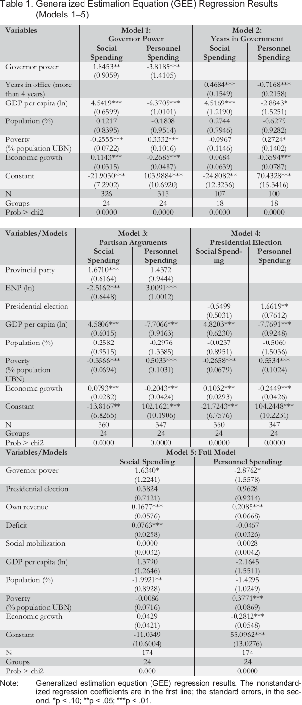
The percentage of the budget allocated by the provinces to social spending varies widely, with the lowest value (7.2 percent in Entre Ríos) being 5.6 times smaller than the highest (40.1 percent in San Luis). The mean for all provinces between 1993 and 2009 is 16.3 percent, and the standard deviation is 5.77 percent. The mean values for the entire series for San Luis and the city of Buenos Aires are marginally higher than 28 percent. These values are almost three times larger than those of the provinces at the other end of the distribution, such as Córdoba and Entre Ríos (figure 1).
Social Spending by Province, 1993–2009
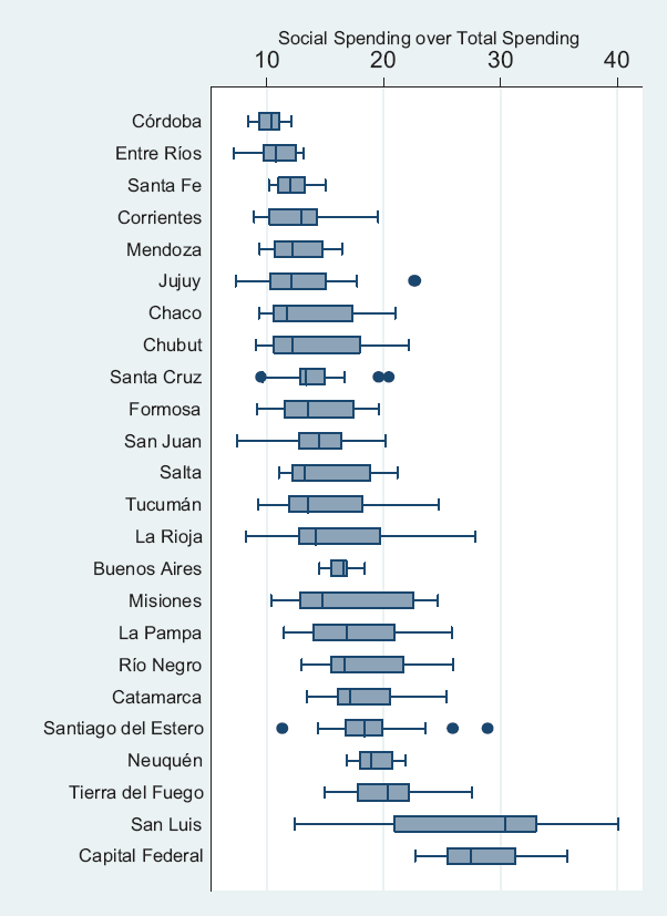
Strikingly, the differences between political parties with regard to social spending in the provinces are minimal. For instance, mean social spending was 15.66 percent for the PJ and the 16.32 percent for the UCR – only a 0.66 difference. Provincial parties, however, had a slightly higher mean (figure 2).
Social Spending by Party, 1993–2009
Regression Analysis
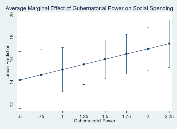
The results of the regression models, reported in Table 1, support our main theoretical expectations. First, electorally secure governors tend to allocate a larger share of the provincial budget to social spending. Controlling for third variables, a one-point increase in the governors’ electoral and legislative power increases social spending by 1.85 percent (model 1). The coefficient is statistically significant at the 0.05 level. Figure 3 reports the predicted average marginal effect (with confidence intervals) of the previously fitted model. Controlling for third variables, we can see a positive marginal effect of gubernatorial power on the dependent variable.
Average Marginal Effect of Gubernatorial Power on Social Spending
I also measure electoral security in government with the number of years in office. Although this variable is not statistically significant in explaining changes in social spending, its coefficient is positive, robust, and statistically significant when the number of years in government is greater than four (more than one term in office). In model 2 we can see that after the first term and controlling for third variables, each additional year in office represents an average increase of 0.5 percent in social spending (statistically significant at the 0.001 level). 9 After the second term (more than eight years in government), the coefficient for social spending is positive and rises to 1.4 percent (statistically significant at the 0.001 level and identical in different model specifications). This reinforces the argument that governors increase social spending when they are electorally secure and have been in office for several years.
If we consider that a governor can typically govern for two consecutive terms of four years, at the end of a governor's tenure the typical governor will have increased social spending by about 2 percent.
I compare these results with those of personnel spending as a percentage of the total provincial budget. In line with our theoretical expectations, a one-point increase in governors’ electoral and legislative power in model 1, while controlling for other variables, substantially decreases personnel spending by 3.8 percent (statistically significant at the 0.01 level). An extra year in government decreases personnel spending by 0.25 percent (statistically significant at the 0.01 level; these results are not reported in the table in order to save space); after four years in office, the coefficient in model 2 becomes even more robust (-0.7 percent; statistically significant at the 0.01 level).
Substantive results remain almost identical in the PCSE models and quite similar in the lagged dependent variable models (see Tables 2 and 3 in the Appendix). The number of years in government and partisan fragmentation produce the same substantive results in all model specifications. The coefficient for gubernatorial electoral and legislative power stays the same in the PCSE and lagged dependent variable models but loses statistical significance in model 1 in Table 3. Including a lagged dependent variable seriously diminishes the number of observations in some models (as Hecock suggests; 2006: 956), so these results should be interpreted with care.
Some of the other arguments in the literature also receive empirical support. The level of party system fragmentation negatively affects social spending but has a positive effect on personnel spending. In model 3 controlling for the usual variables and increasing the effective number of provincial parties by 1 percent decreases social spending by 2.5 percent but increases personnel spending by 3 percent (all coefficients are statistically significant.)
In model 3 we can see that, controlling for third variables, provincial parties spend 1.7 percent more on social matters than the other parties (the PJ and the UCR) (this coefficient is not statistically significant in the PCSE model). With regard to personnel spending, there are no statistically significant results. These results and those in figure 2 indicate that the type of party in government is not relevant for explaining changes in the overall percentage of social spending. This finding is similar to that of Huber, Mustillo, and Stephens (2008: 431, 433).
Another interesting finding in model 4 is that governors do not appear to reduce social spending in election years (this coefficient is not statistically significant) but in fact seem to increase personnel spending (the coefficient for personnel spending is statistically significant only in model 4 of Table 1; none of these coefficients reach the standards of statistical significance in PCSE).
Some structural controls seem relevant for explaining social spending. Richer districts (those with larger values of GDP per capita) tend to allocate more social spending. Results are inconsistent across different models for poverty rates (the coefficient does not always reach levels of statistical significance). 10 The main results for social and personnel spending remain fundamentally unchanged in model 5 in the GEE and PCSE regressions (although the coefficient for gubernatorial power loses statistical significance in the lagged dependent variable model). Model 5 contains the main variables of models 1–4 and the usual controls. Some variables were not included in the full model because of high collinearity with other variables. These results should be interpreted with caution, though, since the number of observations decreases substantially once all the controls have been introduced and because some standard errors have high values.
Arretche, Schlegel, and Ferrari (2016: 94–95) provide individual-level data showing how individual income and regional identities affect preferences for centralization or decentralization of authority in Brazil. Further studies could use individual-level data to test preferences for different types of spending across regions in federal countries.
Social mobilization does not appear to influence either social or personnel spending. I also do not reach any substantial conclusions regarding fiscal determinants. The results indicate that wealthier districts (those with more own income) tend to have higher levels of social spending as well as higher levels of personnel spending. Increases in fiscal provincial deficits seem to be positively associated with slightly more social and slightly less personnel spending (although the coefficient for the latter is not statistically significant).
The R-squares for the five different PCSE models oscillate between 28 percent and 47 percent. These R-squares indicate that we still need better theories, models, and data to further understand the determinants of social spending. Case studies may help us to better understand how these variables operate and to identify potential idiosyncratic factors that affect social spending. In the next section I briefly explore three cases that could guide further in-depth analysis of the Argentine case.
Three Cases: Buenos Aires, San Luis, and Córdoba
I selected Buenos Aires province as one of the cases because it offers high variation across time of the main variables and because of its socio-economic and political relevance. The province comprises more than a third of the country's population and is economically and politically the most important district in Argentina. Here, I briefly discuss the evolution of government spending during Felipe Solá's tenure (2002–2007) as the governor of Buenos Aires Province. 11 Upon taking up the governorship following Carlos Ruckauf's resignation, Solá did not have the support of the legislature, did not control the powerful apparatus of the Buenos Aires faction of the PJ, and faced strong opposition in 22 of the 29 most populated municipalities of the suburbs of Buenos Aires. Eduardo Duhalde, the province's former governor and strongman, and his allies controlled all these political resources. In the legislature, the divisions Solá faced between the Kirchnerist (President Kirchner allies) and Duhaldist (Duhalde allies) factions of the PJ were so intense that he threatened to resign.
Carlos Ruckauf governed from 1999 to 2002, the year in which he resigned to take over as Minister of Foreign Affairs under the presidency of Eduardo Duhalde. Felipe Solá followed him as governor.
Furthermore, he inherited a cabinet appointed by his predecessor. Despite appointing loyal partisans to key positions in the provincial administration (general secretariat and secretary of government) and in politically sensitive areas, such as security and justice (controlling the police) and labor (negotiating with the unions), areas dealing with economic affairs (Ministry of Economy and Public Works), production, health, and education, as well as the influential provincial bank, largely remained in the hands of politicians linked to the former governor.
As we would expect, personnel spending reached historically high levels at the beginning of Solá's tenure: 53.5 percent of the budget in 2002 compared to the province's 1993–2009 average of 49 percent. Meanwhile, social spending dropped to 15 percent, one of its lowest levels during the same period. During his second term in office, Solá sought to increase his influence in the provincial legislature by forming his own legislative delegation and curbing the influence of Peronism from the suburbs of Buenos Aires. By 2005, Solá had the support of Duhaldist senators and of the head of the lower chamber. This enabled Solá to increase the cohesion within his cabinet and contain Peronist disputes in the legislature. He also appointed his own cabinet with loyal ministers (mostly from the provincial interior) and promoted second-line officials to important government positions in the areas of health, education, human development, and environment (Interview with former governor Felipe Solá, 20 December 2016). In the end, Solá amassed so much power, that he tried to run for reelection for a third term even though the provincial constitution bans doing so. As we would anticipate, during his second term, Solá significantly decreased personnel spending by almost 10 percentage points (reaching 43.7 percent in 2005) and increased social spending by 2 percentage points (reaching almost 17 percent in 2007).
I picked San Luis – a small, sparsely populated province of 432,000 inhabitants (according to the 2010 census) – as another case because its provincial government allocates the highest average share of its budget to social spending nationwide. In 1983, after the military dictatorship, Adolfo Rodriguez Saá (PJ) was elected governor by a narrow margin (3,873 votes), receiving 40.5 percent of the vote compared to the 37.3 percent obtained by his Unión Cívica Radical (UCR) rival. In that election, however, the UCR won the presidential vote (48.6 percent), the election for federal deputies (45.5 percent), and the mayoral elections in the province's two main cities (San Luis and Villa Mercedes).
As we would expect under conditions of high electoral competition, personnel spending reached very high values in San Luis, accounting for 76 percent of the budget in 1983. Rodríguez Saá compensated electoral allies and used positions in office to co-opt PJ dissidents and the opposition. He came to power with the help of various PJ factions but began to incorporate allies into his party and co-opt the opposition shortly after taking office. He first co-opted key dissident Peronists from the list that lost the primaries and then critical political figures from opposition parties, such as the Liberal Democratic Party (Bianchi 2013: 140).
Adolfo Rodriguez Saá was elected five times, each time with more than 50 percent of the vote (in 1995 he won with 72 percent). This was possible because he amended the provincial constitution in 1987 in order to provide himself with the possibility of indefinite reelection. His amendments also enabled the overrepresentation of interior districts (which massively supported him) in the newly created provincial senate – a move that secured him control over the legislature.
Adolfo Rodriguez Saá only left office when he was appointed interim president of Argentina in 2001. He was replaced in office by his vice governor, who later resigned, thus allowing his brother, Alberto, to successfully run for office. Alberto Rodriguez Saá was elected with 90.1 percent of the vote in 2003 and reelected with 86.3 percent in 2007. 12
The functioning of the political regime in the province of San Luis is not the main topic of this article. It is worth noting that the democratic “quality” of several of the province's institutions is questioned by the opposition, various scholars, and parts of the local and national media. On the contrary, other analysts argue that stability in government generated benefits, mostly in the second ministerial lines, where there has been significant stability in office and comparatively high bureaucratic quality.
On average, San Luis governors took up office with 60 percent of the vote and controlled 63 percent of the seats in the local legislature (this was as high as 76 percent in 2003). Therefore, these governors enjoyed enormous power over their cabinets, the legislature, and other government institutions. Electoral competition was low during this period: the effective number of parties (votes) for the governors’ election (1983–2003) diminished from 3.03 in 1983 to 1.22 in 2003 (the lowest value at the national level, followed by Santa Cruz [1.72] and Formosa [1.74]).
In line with our theoretical expectations, these governors – who amassed significant political power and stability over 33 years in office – reduced personnel spending by more than 38 percentage points, from 76 percent of the budget in 1983 to 37.6 percent in 2004 (Bianchi 2013: 139). Meanwhile, they increased social spending by 25 percentage points, from 12 percent in 1996 to 37 percent in 2007 (data are available only for these years).
The San Luis governors invested heavily in social infrastructure, especially in housing. Their administrations built 43,202 new houses between 1983 and 2000, granting housing to a third of the province's population. According to Bianchi (2013: 159), San Luis had the second-lowest amount of investment in housing in 1983 (after La Rioja), representing 0.7 percent of national housing funds. However, by 1991, San Luis was seventh highest with 5.1 percent. The province's investment in water infrastructure also skyrocketed, with the provincial government building 2,500 km of aqueducts between 1983 and 2003 (before 1983, the province only had 30 km of aqueducts). 13 In 2003 the San Luis government launched the Social Inclusion Plan, its most ambitious social initiative. Any unemployed person over 18 years of age could apply for this universal access plan. By 2005, the initiative had about 45,000 beneficiaries (about one-third of the economically active San Luis population and 2.2 times the number of state employees (Behrend 2007: 13)), accounting for 18 percent of the provincial budget (Bianchi 2013: 164).
The average number of kilometers of paved roads per year increased from 17.42 km for the period 1976–1983 to 89.3 km for 1983–1991 (Bianchi 2013: 159).
I chose Córdoba as the other case given its status as Argentina's second most important province in socioeconomic terms. It also has the lowest mean social spending levels in the country (10.3 percent of the budget).
The UCR won comfortably in Córdoba at the provincial and municipal levels in 1983. Eduardo Angeloz was elected governor with 55.8 percent of the vote, with his nearest rival only securing 39.2 percent. During his first term, Angeloz reformed the provincial constitution, allowing him to run for reelection. He was subsequently reelected in 1987 (by a small margin) and again in 1991. The amended constitution also introduced the so-called “governability clause”, which granted the winning party an automatic majority of 36 seats (out of a total of 66). In Córdoba this was a period of stable rule for the incumbent UCR party, whose governors obtained an average 51 percent of the vote and controlled nearly 58 percent of the seats in the provincial legislature. As is to be expected, social spending was fairly stable (1 percent standard deviation) and closer to the national mean during these years, accounting for 11 percent on average. Despite this, personnel spending also remained high, averaging 52 percent with a standard deviation of 2.6 points.
In 1999, as a result of a deep economic crisis and severe adjustment policies that divided the party and plunged popular support, the UCR lost its first election after four consecutive terms in office. Supported by President Menem (PJ), the winning PJ candidate for the governorship, José Manuel De la Sota, formed a center-right coalition called Union for Córdoba, comprising the PJ, the Democratic Center Union, Action for Change, and the Christian Democracy of Córdoba.
At the beginning of his first term in office, and partly as a result of increased political competition and a fragmented and diverse electoral coalition, De la Sota increased personnel spending from 46.7 percent of the budget in 1998 to a peak of 52 percent in 2000. Once he had consolidated his power, he began to reduce personnel spending, taking it down to 36.6 by 2004.
Social spending, on the contrary, plummeted to an average of 9 percent of the budget under De la Sota, reaching a historical low of 8.4 percent in 2001, the year of an acute economic crisis in the country. In fact, the average share of the budget allocated to social spending under the PJ administrations in Córdoba (1999–2009) was 9.9 percent. In contrast to the personnel-spending trend, social spending increased from 8.4 percent in 2001 to 10.7 in 2009. Between 2001 and 2004 the provincial government constructed over 200 new schools (377,701 m 2 of new school surface) through Plans 100 and 110 New Schools at a cost of ARS 537 million and 4,180 new houses. It also created the Municipal Assistance Program (PAM) to strengthen nutrition programs, medical care, and social assistance at the municipal level (Nazareno, Mazzalay, and Cingolani 2012: 262–263).
In short, these cases show that the main variables seem to move in the expected direction, especially in the cases of Buenos Aires and San Luis. More case studies can be valuable in complementing quantitative analyses and providing a more detailed and complex understanding of the relationships between variables.
Discussion
The results of the regression models and the analyses of the cases indicate that the more secure governors are electorally and the longer they have been in office (particularly those who have completed a first term), the more they tend to invest in social spending. Governors with strong political support are under less pressure from their coalition partners to engage in particularistic spending, reduce turnover in executive positions by appointing loyal staff in key cabinet posts, and have more control of the bureaucracy and greater freedom to decide how to spend the provincial budget. Under these conditions, governors increase social spending on goods that benefit a broader number of voters in order to expand their electoral base (as well as to show their achievements in office and advance their political careers outside the province).
By contrast, electorally weak governors, especially those at the beginning of their terms in office and those with less legislative support, need to distribute positions among their core electoral allies and build up political support to govern. On top of that, they face more cabinet divisions and greater resistance from the bureaucracy. This results in them increasing personnel spending, which negatively impacts on social spending. I therefore contend that putting together an electoral and a governing coalition with low electoral and legislative support, within the context of fragmented party systems, has a negative effect on social-spending levels. The proposed theoretical argument and the empirical evidence I found seeks to further specify the effect of electoral competition on social spending by including not only electoral expectations but also governing dynamics. Future research could further explore this connection using cases from other countries.
I also believe that the positive relationship between electoral security and social spending I find in this study has not only important implications for the theoretical discussion on the effects of electoral competition or stability but also fundamental implications for the social policies that define development strategies, especially in developing countries and federal democracies.
Footnotes
Appendix
PCSE Regression Results (Models 1 to 5)
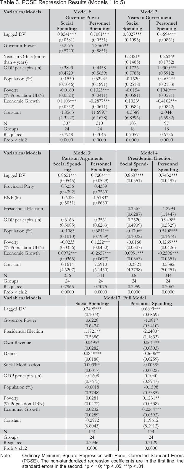
| Variables/Models | Model 1: Governor Power | Model 2: Years in Government | ||
|---|---|---|---|---|
| Social Spending | Personnel Spending | Social Spending | Personnel Spending | |
| Lagged DV | 0.8541 *** (0.0581) | 0.7081 *** (0.0531) | 0.8027 *** (0.1095) | 0.6694 *** (0.0861) |
| Governor Power | 0.2595 (0.5720) | -1.8569 ** (0.8851) | ||
| Years in Office (more than 4 years) | 0.2421 * (0.1485) | -0.2636 * (0.1752) | ||
| GDP per capita (ln) | 0.3893 (0.4729) | 0.4458 (0.5659) | 0.1726 (0.7785) | 1.9300 *** (0.5912) |
| Population (%) | -0.1550 (0.1046) | 0.3294 * (0.1891) | -0.1520 (0.2518) | 0.4632 ** (0.2153) |
| Poverty (% Population UBN) | -0.0160 (0.0324) | 0.1323 *** (0.0411) | -0.0154 (0.0581) | 0.1949 *** (0.0571) |
| Economic Growth | 0.1108 *** (0.0352) | -0.2877 *** (0.0611) | 0.1023 * (0.0584) | -0.4102 *** (0.0842) |
| Constant | -1.8563 (4.3227) | 11.6997 * (6.1678) | -0.3389 (6.8996) | -2.0446 (6.5932) |
| N | 307 | 310 | 103 | 97 |
| Groups | 24 | 24 | 18 | 18 |
| R squared | 0.7948 | 0.7045 | 0.7057 | 0.6756 |
| Prob > chi2 | 0.0000 | 0.0000 | 0.0000 | 0.0000 |
| Variables/Models | Model 3: Partisan Arguments | Model 4: Presidential Election | ||
|---|---|---|---|---|
| Social Spending | Personnel Spending | Social Spending | Personnel Spending | |
| Lagged DV | 0.8651 *** (0.0545) | 0.7204 *** (0.0529) | 0.8687 *** (0.0551) | 0.7432 *** (0.0497) |
| Provincial Party | 0.3256 (0.4392) | 0.4339 (0.7560) | ||
| ENP (ln) | -0.6027 (0.5051) | 1.5183 * (0.8630) | ||
| Presidential Election | 0.3565 (0.6287) | -1.2994 (1.1447) | ||
| GDP per capita (ln) | 0.3166 (0.5085) | 0.3561 (0.6263) | 0.2520 (0.4939) | 0.9498 * (0.5329) |
| Population (%) | -0.1083 (0.1010) | 0.3811 ** (0.1939) | -0.1706 * (0.1022) | 0.5408 *** (0.1674) |
| Poverty (% Population UBN) | -0.0233 (0.0336) | 0.1222 *** (0.0450) | -0.0168 (0.0307) | 0.1269 *** (0.0426) |
| Economic Growth | 0.0972 *** (0.0365) | -0.2657 *** (0.0677) | 0.0951 *** (0.0363) | -0.2596 *** (0.0651) |
| Constant | 0.1614 (4.6207) | 7.5910 (6.1450) | -0.3821 (4.3798) | 3.5382 (5.0251) |
| N | 336 | 344 | 336 | 344 |
| Groups | 24 | 24 | 24 | 24 |
| R squared | 0.7965 | 0.7075 | 0.7959 | 0.7067 |
| Prob > chi2 | 0.0000 | 0.0000 | 0.0000 | 0.0000 |
| Variables/Models | Model 7: Full Model | |
|---|---|---|
| Social Spending | Personnel Spending | |
| Lagged DV | 0.7495 *** (0.1074) | 0.6899 *** (0.0869) |
| Governor Power | 0.6228 (0.6474) | -1.0817 (0.9410) |
| Presidential Election | 1.1721 ** (0.5386) | -2.2400 * (1.1833) |
| Own Revenue | 0.0495 * (0.0282) | 0.0617 ** (0.0303) |
| Deficit | 0.0849 *** (0.0188) | -0.0606 ** (0.0259) |
| Social Mobilization | 0.0039 ** (0.0017) | -0.0038 * (0.0022) |
| GDP per capita (ln) | -0.1608 (0.7675) | 0.1040 (0.8947) |
| Population (%) | -0.6018 (0.3748) | -0.1598 (0.5385) |
| Poverty (% Population UBN) | 0.0281 (0.0472) | 0.1231 ** (0.0538) |
| Economic Growth | 0.0232 (0.0289) | -0.2264 *** (0.0592) |
| Constant | -0.2972 (6.8043) | 11.9612 (8.2912) |
| N | 174 | 174 |
| Groups | 24 | 24 |
| R squared | 0.7946 | 0.7129 |
| Prob > chi2 | 0.000 | 0.0000 |
Note: Ordinary Minimum Square Regression with Panel Corrected Standard Errors (PCSE). The non-standardized regression coefficients are in the first line, the standard errors in the second.
p < .10;
p < .05;
p < .01.