
Abstract
We study a quantum dot light-emitting diodes (QD-LEDs) subject to filtered optical feedback, where the filter is characterized by a mean frequency Ω m and a filter width λ. In the limit of a narrow filter (λ = 0), the QD-LED equations reduce under some conditions to the equations for a QD-LED with optical feedback, whereas they become the Lang Kobayashi equations in the limit of an unbounded filter width (λ > 0). Through simulations based on the rate equations for a QD-LED with filtered external optical feedback modes, we show that the output’s nonlinear dynamical system attractors can be controlled through the filter parameters: the filter’s spectral width λ and its central frequency Ω m. This is illustrated for a filter-induced global bistability.
Introduction
In nanotechnology, nanoparticles are classified by their size (in the range of 1–100 nm) and properties. Nanocrystals are described as having at least one dimension of less than or equal to100 nm and single crystalline. Quantum dots (QDs), also known as nanocrystals, are a nontraditional type of semiconductor with limitless applications as an enabling material across many industries. 1 The quantum dots, which can also be called artificial atoms, are nanometer-scale “boxes” that selectively hold or release electrons. These semiconductors range in size from 2 nm to 10 nm in diameter, which consist of 10–50 atoms. From a few hundred to a few hundred thousand atoms, QDs bridge the gap between single atoms and solid state, and because of this, they exhibit a combination of atomic and solid-state properties. The emission wavelength, or the color emitted, of QDs depends on the size, and using simple chemistry with semiconductor nanocrystals, the color can be precisely controlled. Light-emitting diodes (LEDs) have been created and produced in various colors from QDs. 2
Semiconductor LEDs are very efficient in transforming electrical energy to incoherent light. Incoherent light is created in the LED by recombination of electron–hole pairs, which are generated by an electrical pump current. This recombination results in spontaneous emission of photons (light) and is amplified by multi emission. These photons should be allowed to escape from the device without being reabsorbed. On the down side, quantum dot light-emitting diodes (QD-LEDs) are known to be very sensitive to optical influences, 3 especially in the form of external optical feedback from other optical components (such as mirrors and lenses) and via coupling to other systems. Depending on the exact situation, optical feedback may lead to many different kinds of output dynamics, from increased stability 4,5 all the way to complicated dynamics; for example, a period doubling cascade to chaos, 6 torus break-up, 7 and a boundary crisis 8 have been identified. See the study of Fischer et al. 9,10 as entry points to the extensive literature on the possible dynamics of output with optical feedback.
A main concern in this article is to achieve stable, and possibly tunable, QD-LED operation. One way of achieving this has been to use filtered optical feedback (FOF) where the reflected light is spectrally filtered before it reenters the QD. As in any optical feedback system, important parameters are the delay time and the feedback strength. Moreover, FOF is a form of coherent feedback, meaning that the phase relationship between outgoing and returning light is also an important parameter.
The interest in the FOF QD-LED is due to the fact that filtering of the reflected light allows additional control over the behavior of the output of the system by means of choosing the spectral width of the filter and its detuning from the light frequency. The basic idea is that the FOF QD-LED produces stable output at the central frequency of the filter, which is of interest, for example, for achieving stable frequency tuning of QD-LEDs for the telecommunications applications.
QD-LED model with FOF
Depending on the model of Marino et al. 11 of LED, the QD-LED with external FOF is modeled, here, mathematically by four equations. Before going into the model, one must refer that this type modeling was accepted since we go into dimensionless modeling and it gives a behavior similar to an experimental one. 12 A new modeling for QD-LED appear in our recent work 13 may accepted at any case.
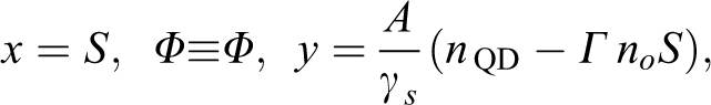
Depending on the model of Marino et al., 11 the rate equations for the (complex) electric field E and the (real) number of carriers in QDs n QD and in the Wetting Layer (WL) n wl can be written as:


Here,
For a three-level atomic system where the transition is homogeneously broadened, it can be shown from the Einstein relation that: 14

Here, A is the spontaneous emission rate into the optical mode, no is the initial carrier occupation number of the QDs, and Γ is the optical confinement factor. In such a case, the spontaneous emission coefficient and absorption coefficient possess identical lineshapes. For realistic QD material system, both the QD and WL states can be inhomogenously broadened. Population distributions in both WL and QD are taken into account explicitly in order to determine the correct relation between absorption and spontaneous emission spectra. E
sp
(t) is the stochastic function corresponding to the zero-mean random field for spontaneous emissions. The field has the relation of

where β is the spontaneous emission factor, VD the normalization QD volume, D(w) the normalized lineshape function, and p(w) the density of photon for the nonuniform QD.
Furthermore, when we investigate the fundamental dynamics of instability and chaos in nonlinear systems, we can treat the deterministic terms with considering statistical noises.
A straightforward way to let a QD-LED operate in a single longitudinal mode is by filtering the feedback light. Light with certain frequencies can pass the filter, while other frequencies are filtered (Figure 1). In equations (1) to (3), a delay term

Schematic setup of the considered QD-LED device with filtered optical feedback. QD-LED: quantum dot light emitting diode.
For simplicity, suppose that we build a new function


where Λ is the half width at half-maximum (HWHM) of the spectrum and


Here
For numerical purposes, it is useful to rewrite equations (8) to (13) in dimensionless form. To this end, we introduce the new variables:
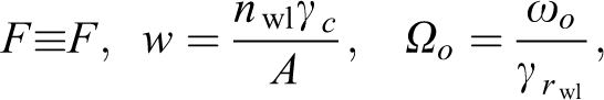
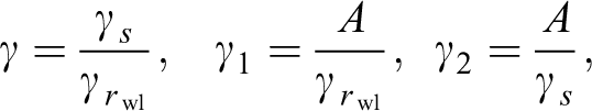
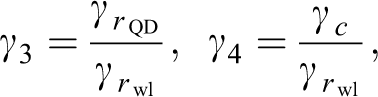


where
Equation (14) describes the time evolution of the real-valued slowly varying electric field amplitude and equation (15) describes the phase of the emission light. Equations (16) and (17) describe normalized number of carriers within the QD and WL. In equation (15) the material properties of the QD-LED are described by the linewidth enhancement factor α (which quantifies the amplitude-phase coupling or frequency shift under changes in number of carriers 23 ), the ratio between the carrier injection and the photon nonradiative decay rates, and the dimensionless pump parameter δo . Time is measured in units of the inverse photon nonradiative decay rates of 10−11 s. Throughout, we use values of the QD-LED parameters given in Table 1.
Numerical parameters used in the simulation unless stated otherwise.

The FOF loops enter equations (14) and (15) as feedback terms Ɛ 1 Fc (t) and Ɛ 2 Fs (t) with normalized feedback strengths Ɛ 1 and Ɛ 2 of the normalized filter terms Fc (t) and Fs (t). In general, the presence of a filter in the system gives rise to an integral equation for the filter field. However, in the case of a Lorentzian transmittance profile as assumed here, derivation of the respective integral equation yields the description of the filter fields by a delay differential equations (18) and (19); see the study of Yousefi and Lenstra 19 for more details. The filter loop is characterized by a number of parameters. As for any coherent feedback, we have the feedback strength Ɛi , the delay time θ, and the feedback phase Cp of the filter field, which is accumulated by the light during its travel through the feedback loop. Hence, Cp = Ω 0θ. Owing to the large difference in time scales between the optical period 2π/Ω0 and the delay time θ, one generally considers θ and Cp as independent parameters.
To investigate the dynamics, numerical integration of the rate equations is performed using a modified Runge–Kutta method of the fourth order. Throughout the simulations, the internal QD-LED parameters were fixed, while the solitary frequency was biased around 0.2/π, τ = 0.05, and central frequency Ωm = 0.02/π. The results are presented in terms of bifurcation diagram where the behavior of the output of the QD-LED system is depicted as a function of the HWHM of the spectrum, as shown in Figure 2. In order to allow quick overview of all the different types of dynamics that may occur during a full scan of the HWHM of the spectrum, a visualization technique very similar to that of the time series, attractor’s section representation is employed at inter-spike interval. A plane is defined in a three-dimensional phase space, chosen such that all the possible to it as shown in Figure 3(a) to (d).

Bifurcation diagram summarizing different dynamics that occur when HWHM is varying. HWHM: half width at half-maximum.

In summary, as the HWHM is increased, we observe the transition between the steady state and oscillatory states at smaller bias value, the system fires less spikes and tends to exhibit small amplitude.
In Figure 4, the system shows multi-chaotic behavior with one-stable region between the frequencies which are about −0.09 to −0.06 not apart. The one-stable region is centered on the filter center and the solitary optical mode island of fixed points, respectively. In Figure 4, the bifurcation diagram for the filter-induced global bistable interval is shown. Going from right to left in Figure 4 (increasing solitary optical mode), the system is initially in a state of chaotic attractors and then it passes through a cascade of period doubled with small amplitude, self-oscillations (limit cycles), achieving the steady state before reprising itself again. When the locking range of the filter is reached, the global bistability appears.

External filtered modes
We restrict ourselves to the study of “fixed points” or the so-called external filtered modes (EFMs) and the bifurcations associated with these states, which occur when the filter parameter λ(Λ) is varied. Although the equations for the fixed points have been written many times before, 19 they haven’t been analyzed for QDs in a concise way yet. In this section, we analyze the QD rate equations of the EFM.
The basic solution of rate equations is the trivial solution (E; n QD; n wl; F) = (0; 0; P; 0) of equation (8). When this basic solution is stable, there is no optical mode activity; the output is off. Increasing the value of the pump P, it becomes unstable at the light threshold P = 0: the output starts optical mode and the so-called EFMs are formed. Such solutions have constant intensities and population, and a phase that depends linearly on time:

Note here, that Ωs is the detuning of the frequencies of E and F, where

where:

and

The final form of EFMs is equation (22); this equation is similar to the EFMs of a conventional laser, with the addition of the first term in the denominator and the dependence on two sets of parameters. Equation (21) is a transcendental and implicit equation that allows one to determine all possible frequencies Ωs of the EFMs for a given set of filter parameters. More specifically, the sought frequency values Ωs of the FOF QD-LED can be determined from equation (21) numerically by root finding; for example, by Newton’s method in combination with numerical continuation. The advantage of the formulation of equation (21) is that it has a nice geometric interpretation: Ωsθ is a function of Ωs that oscillates about fixed value. More precisely, when Ωo is changed over 2π, the graph of Ωsθ sweeps out over the area.
Once Ωs is known, the corresponding values of the other state variables of the EFMs can be found from:


Note that in this manner each mode of single-frequency operation of the output corresponds to a fixed point. The solutions to equation (9) can be obtained by graphical methods, from which the intersection of the straight line Ω sθ with the oscillating right-hand side of equation (9) can be found. Thus, the solutions of equation (9) correspond to the intersections of f (Ω s ) and g(Ω s ), and bifurcations of EFMs occur when both f (Ω s ) = g(Ωs ) and f ΩS = gΩ S . A combination of these two requirements will lead to our bifurcation results. In Figure 5, the functions f and g are plotted as Ωf is increased.

Plot of f and g as functions of Ωf as the parameter is increased. (a) Only one EFM exists. (b) Two EFMs are formed in a saddle-node bifurcation. (c) There are three EFMs. EFM: external filtered mode.
Figure 5 shows an example of the solutions of equation (8) as intersection points (blue line) between the oscillatory function ΩS (ωs ) and the diagonal (the straight line through the origin with slope 1); see also the study of Yousefi and Lenstra. 19 This means that an EFM is, in fact, uniquely determined by its value of ωs . Furthermore, Figure 5 represents all the relevant geometric information needed to determine and classify EFMs. Notice that in this specific example, the EFMs are separated into three groups. This geometric picture is very similar to that of the single FOF laser, 19 but there is an important difference. For the FOF QD-LED, considering the attractor of the carrier’s number function as the detuning of the frequencies in equation (11). Figure 6 shows a small cycle in Figure 6(a), (b), and (d) at the same index of frequency and different indexes for large cycles.
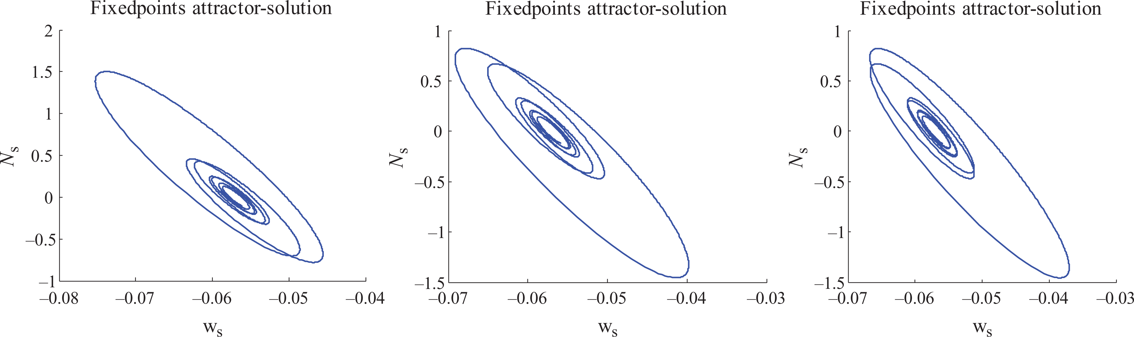
Fixed-point attractor solution. Corresponding with Figure 5.
The results of the fixed-point analysis are presented in terms of bifurcation maps where the behavior of the instantaneous frequency of the QD-LED system is depicted as a function of the solitary output frequency. Figure 7 shows the fixed points in the (ΩS (ΩO ), ΩO )-plane, where Ωs is the frequency of the compound QD-LED system. It is precisely in these intervals that one should expect filter-induced bistability. This can be studied by investigating the dynamical behavior of the system. Note, in this respect, that nothing has been said yet about the stability of the fixed points. In fact, it is well known that feedback has a large destabilizing influence on the system in general, but in the case of filtering, one may expect some type of stabilization to occur.

The fixed points in the (ΩS (ΩO ), ΩO ) plane. The dash line ΩO = Ωf indicates the filter center. The fixed points are created and annihilated in saddle node bifurcations as the solitary QD-LED frequency is changed. QD-LED: quantum dot light emitting diode.
Conclusion
The main conclusion we draw from our simulations is that the filter detuning can be used for the controlled access to the various different dynamics. For the bifurcation diagram parameters studied, most of the dynamics show, sometimes in limit cycles and double periodic, large regions of chaotic dynamics. We have theoretically analyzed the influence of a relatively narrow frequency filter (HWHM = 0.03) while the solitary frequency is biased around 0.2/π, τ = 0.05, and central frequency Ωm = 0.02/π on the deterministic nonlinear dynamics of a semiconductor QD-LED with filtered external optical feedback.
It should be mentioned that in our numerous experiments, we have observed many more interesting dynamical attractors, like limit cycles, quasi-periodicity, and strange attractors, which are not addressed in this article.
Footnotes
Declaration of conflicting interests
The author(s) declared no potential conflicts of interest with respect to the research, authorship, and/or publication of this article.
Funding
The author(s) received no financial support for the research, authorship, and/or publication of this article.