
Abstract
We study game equilibria in a model of production and externalities in network with two types of agents who possess different productivities. Each agent may invest a part of her endowment (it may be, for instance, time or money) in the first of two time periods; consumption in the second period depends on her own investment and productivity as well as on the investments of her neighbors in the network. Three ways of agent’s behavior are possible: passive (no investment), active (a part of endowment is invested), and hyperactive (the whole endowment is invested). For star network with different productivities of agents in the center and in the periphery, we obtain conditions for existence of inner equilibrium (with all active agents) and study comparative statics. We introduce adjustment dynamics and study consequences of junction of two complete networks with different productivities of agents. In particular, we study how the behavior of nonadopters (passive agents) changes when they connect to adopters (active or hyperactive) agents.
Introduction
Social network analysis became an important research field, both as a subject area and as a methodological approach applicable to analysis of interrelations in various complex network structures, not only social but also political, economic, and urban. There is also a permanent exchange of ideas among researchers doing network analysis in social sciences, biology, physics, computer science, engineering, and many other fields. 1 A special place in this multidisciplinary research activity is played by methods of network economics and network games. 2 –7 Economic models assume that agents/actors in network act as rational decision makers whose actions are results of solving optimization problems, and the profile of actions of all agents in the network is a game equilibrium. Decision of each agent is supposed to be influenced by behavior (or by knowledge) of her neighbors in the network. Such approach, despite being, in some sense, one sided, is found to be very productive analytically and allows finding new perspectives which can be further elaborated by use of other approaches in the multidisciplinary framework.
In majority of research on game equilibria in networks, 2,8 –10 the agents are assumed to be homogeneous (except their positions in the network), and the problem is to study the relation between the agents’ positions in the network and their behavior in the game equilibrium. The models demonstrate that the agents’ behavior and well-being depend on their position in the network which is characterized by one or another measure of centrality. Thus, research on equilibria is in a close connection with research focusing on the network structure. For instance, Cinelli et al., 11 Ferraro and Iovanella, 12 and Ferraro et al. 13 consider two types of nodes in a network. Different approaches to describe interrelations in networks are used, for example, intensiveness of interplay between nodes in the study by Ferraro et al. 13 is given exogenously, while in the study by Matveenko and Korolev, 9 it depends endogenously on the agent’s behavior in network, since in the latter work agents’ interplay depends on the externalities created by investments of neighbors in the network.
Diversity and heterogeneity have become an important aspect of contemporary social and economic life (international working teams is a typical example; many other examples are described by researchers of inclusiveness and social cohesion 14 ). Correspondingly, along with accounting for position of agents in the network, an important task is to account for heterogeneity of agents as a factor defining differences in their behavior and well-being. This direction of research is forming in the literature. For example, in the study by Bramoullé et al., 15 agents possess different marginal costs.
In the present article, we add heterogeneity of agents into the Romer's 16 two-period consumption-investment model (where a special case of complete network is considered) and the more general model by Matveenko and Korolev. 9 These models consider situations in which in time period 1, each agent in network, at the expense of diminishing current consumption, makes investment of some resource (such as money or time) with the goal to increase her consumption in period 2. The latter depends not only on her own investment and productivity but also on investments by her neighbors in the network. Total utility of each agent depends on her consumption in the two time periods. Such situations are typical for families, communities, international organizations, innovative industries, and so on. In the framework of the model, questions concerning interrelations between the network structure, incentives, and behavior are studied.
We use the concept of “Nash equilibrium with externalities” similar to the one used by Romer 16 and Lucas. 17 As in the common Nash equilibrium, agents maximize their payoffs (utilities), and in equilibrium, no one agent finds gainful to change her behavior if others do not change their behaviors. However, the agent’s maximization problem under the present concept is such that the agent is not able to change her behavior so “free” as it is allowed by the common Nash equilibrium concept. In some degree, the agent is attached to the equilibrium of the game. Namely, it is assumed that the agent makes her decision being in a definite environment formed by herself and by her neighbors in the network. Though she participates herself in formation of the environment, the agent in the moment of decision-making considers the environment as exogenously given.
Romer’s 16 and Matveenko and Korolev 9 consider only the case of homogeneous (in their preferences and productivities) agents. In the present article, we assume that there are two types of agents with different productivities.
We find conditions under which agent behaves in equilibrium in some definite way, being “passive” (does not invest), “active” (invests a part of the available endowment), or “hyperactive” (invests the whole endowment). We prove that the agent’s utility depends monotonously on her environment and study dependence of the investment on the externality received by the agent. For complete networks, we prove the uniqueness of the inner equilibrium (in which all agents are active).
We study the influence of the nonhomogeneity on the game equilibria. For instance, we show that if in star network the central node (type 1) has a different productivity than the peripheral agents (type 2), an increase of productivity of any of these types always leads to decrease of investment by another type in equilibrium. However, influence of changes in productivity on own investment is ambiguous and depends on the counterpart’s productivity. If productivity of type i is sufficiently low (less than a threshold value), then an increase in productivity of type j
Another question studied in the article is consequences of unification of networks with different types of agents. We study junction of complete networks and find conditions under which the initial equilibrium holds after unification, as well as conditions under which the equilibrium changes. In particular, we study how the behavior of nonadopters (passive agents) changes when they connect to adopters (active or hyperactive) agents.
We introduce adjustment dynamics into the model and study dynamics of transition to the new equilibrium. The dynamics pattern and the nature of the resulting equilibrium depend on the parameters characterizing the heterogeneous agents.
For instance, if complete network 1 with initially active agents of type 1 unifies with complete network 2 with initially passive agents of type 2, and the type 1 productivity is higher than the type 2 productivity by at least a certain threshold value (which we show to be inversely proportional to the number of the first type agents), then there is no transition process: The network stays in the (dynamically unstable) equilibrium in which the first type agents are active and the second type agents are passive. In the opposite case, a transition process starts in the unified network. If productivity of type 2 is higher than the abovementioned threshold but still rather low, then the transition process leads to the stable equilibrium in which the first type agents are hyperactive and the second type agents are active, that is, all agents increase their investment levels. Under a higher productivity of type 2, the transition process leads to a stable equilibrium in which agents of both types are hyperactive.
We show that all these results are in power not only for complete networks but also for a wider class of “cognate” regular (equidegree) networks.
Such kind of results can be useful in analysis of functioning of real social, organizational, economic, and political structures.
The article is organized in the following way. The model is formulated in “The model” section. Agent’s behavior in equilibrium is studied in “Indication of agent’s ways of behavior” section. “Equilibria in complete network with two types of agents” section studies equilibria in complete network with heterogeneous agents. “Adjustment dynamics and dynamic stability of equilibria” section introduces and studies the adjustment dynamics which may start after a small disturbance of initial inner equilibrium or after a junction of networks. “Junction of two complete networks” section studies consequences of junction of two complete networks with different types of agents. “Equilibria in star network with heterogeneous agents” section considers equilibria in star network with heterogeneous agents. The final section is conclusion.
The model
There is a network (undirected graph) with n nodes,

Investment immediately transforms one to one into knowledge which is used in production of good for consumption in the second period,
Preferences of agent i are described by quadratic utility function

where
Production in node i is described by production function

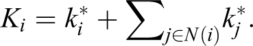
which depends on the state of knowledge in ith node, ki , and on environment, Ki . The environment is the sum of investments by the agent himself and her neighbors

where
We will denote the product
Three ways of behavior are possible: agent i is called passive if she makes zero investment,
Let us consider the following game. Players are the agents


where the environment
Substituting the constrains equalities into the objective function, we obtain a new function (payoff function)

If all players’ solutions are internal

Here

We will use the following notation: I is the unit
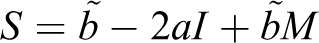
Remark 1.1. System of equation (2) takes the form

where
Here, I is the identity matrix such that
Remark 1.2. Since the matrix
is nonsingular, we can multiply both parts of equation (4) by diagonal matrix

Let us introduce a diagonal matrix

and a vector

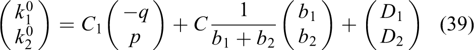
If matrix S is nonsingular, then the unique solution of the system (4) takes the form
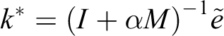
Thus, the equilibrium investments by the agents are defined by their generalized α-centralities in the network. Instead of one α-parameter (as in the common definition of α-centrality), we have here a diagonal matrix α, that is, the heterogeneous agents are characterized by parameters αi depending on their productivities, bi . Notice that two components of centrality (the agent’s position in the network and her exogenous “importance”) influence the equilibrium investment level in the opposite directions.
Theorem 1.1. For complete network, the inner equilibrium exists and unique
Proof. We shall proof that complete network system of equation (4) has a unique solution. It is sufficient to check the nonsingularity of the matrix

Here,
We will prove by induction that for complete network of order n, the determinant of matrix
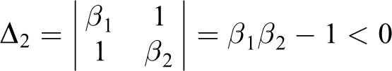
For

Suppose that we have proven the statement for all complete networks of order not higher than n. Let us prove it for the complete network of order
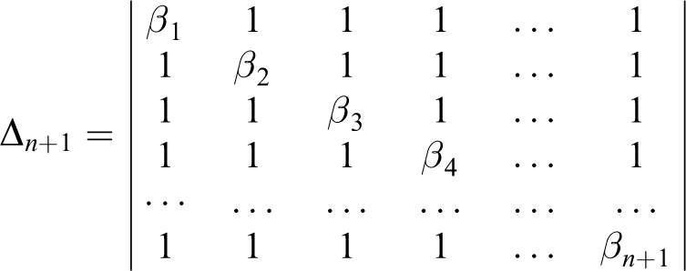
Subtracting the first column from the second column, the second column from the third column,…, the n th column from the

When n is even, then both additives in equation (5) are positive, and when n is odd, they are both negative.
We have proven that for any n, the determinant of matrix
In the inner equilibrium,
Remark 1.3. Notice that in general case (for incomplete networks), the theorem 1.1 is not true. As a counterexample, let us consider the chain of three nodes with matrix
of the form

The determinant of this matrix

becomes 0 under

which is possible under
The following theorem will serve as a tool for comparison of utilities.
Theorem 1.2
Let W*, W** be networks with the same characteristic endowment e; If If If If
Proof. Let
The last statement of the theorem is evident

because for
Indication of agent’s ways of behavior
The following statement plays the central role in analysis of equilibria.
Lemma 2.1. For unproductive agent, necessary and sufficient conditions of different ways of behavior in equilibrium are as follows
1) Agent is passive iff
2) Agent is active iff

3) Agent is hyperactive iff

For productive agent, necessary conditions of different ways of behavior in equilibrium are as follows: 1) Agent may be passive only if
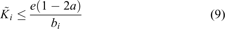
2) Agent may be active only if

3) Agent may be hyperactive only if

Proof. Equilibrium condition for passive agent is

which is equivalent to equations (6) and (9).
The agent is active iff
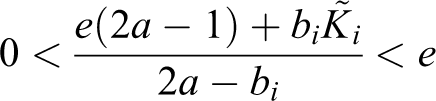
Writing this relation in detail, we obtain equation (7) if agent is unproductive or equation (10) if agent is productive.
Equilibrium condition for hyperactive agent is

which is equivalent to equations (8) and (11). □
Remark 2.1. Pure externality can be interpreted as social influence. Lemma 2.1 shows the values of social thresholds for agent i; achievement of a threshold is needed for a change in behavior. The lemma implies that to turn from passive into active (or from active into hyperactive), an agent with a lower productivity needs a bigger social influence externality than an agent with a higher productivity
We will denote by

Thus

where
Corollary 2.1. For unproductive agent, necessary and sufficient conditions of different ways of behavior are as follows
1) Agent is passive iff

2) Agent is active iff

3) Agent is hyperactive iff

For productive agent, necessary conditions of different ways of agent’s behavior are as follows: 4) Agent may be passive if

5) Agent may be active if

6) Agent may be hyperactive if

Corollary 2.2. (Matveenko and Korolev,
9
corollary 3.4). Agents in a complete network of order
are passive if
are passive or hyperactive if
are passive, activ,e or hyperactive if
Remark 2.2. Evidently,
can be presented as

Notice that formula (18), by itself, does not provide the equilibrium investment of ith agent, because
Formula (18) implies that in equilibrium in complete network (where the environment is the same for all), any agent with a higher productivity invests more (and consumes in the first period less) than any agent with a lower productivity. Formula (18) and the expression for the payoff function,
In lemma 2.1 and corollary 2.1, we provide description of agent’s ways of behavior in terms of pure externality,
Lemma 2.2. In equilibrium, i-th agent is passive iff

i-th agent is active iff

i-th agent is hyperactive iff

Proof. Since

the first-order conditions for the ith agent imply that


But equation (22) is equivalent to equation (19), and equation (24) is equivalent to equation (21). It follows from equation (23) that
which is equivalent to equation (20). □
In any complete network, the environment is the same for all agents. This implies the following corollary.
Remark 2.3
In complete network in equilibrium, agents with the same productivity make the same investments. If all agents have the same productivity, then a homophily takes place: Everyone behaves in the same way.
Remark 2.4
In complete network, there cannot be equilibrium in which an agent with a higher productivity is active while an agent with a lower productivity is hyperactive or when an agent with a higher productivity is passive while an agent with a lower productivity is active or hyperactive.
Speaking about complete network, we will omit index i in notation for the i th agent’s environment, because the environment in complete network is the same for all agents. In other words, K will denote the sum of investments of all agents of complete network.
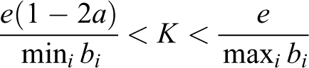
Corollary 2.3. In complete network, equilibrium with all hyperactive agents exists iff
In this case
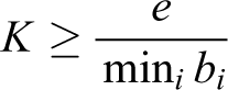
Equilibrium with all active agents exists iff
Equilibrium with all passive agents always exists. In this case,
Proof. Assume that in a complete network, all agents are hyperactive. According to equation (24), it is possible iff

that is iff

Other statements of the corollary follow directly from lemma 2.2. □
Equilibria in complete network with two types of agents
Let a complete network consist of p agents with productivity
Proposition 3.1
In complete network with two types of agents, the following equilibria exist.
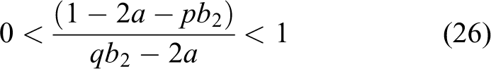
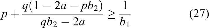
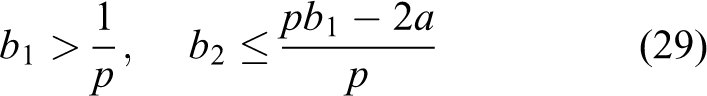
1) Equilibrium with all hyperactive agents exists if 2) Equilibrium in which first type agents are hyperactive and second type agents are active exists if 3) Equilibrium in which first type agents are hyperactive and second type agents are passive exists if 4) Equilibrium in which first type agents are active and second type agents are passive exists if 5) Equilibrium with all passive agents always exists. 6) Equilibrium in which agents of both types are active exists if
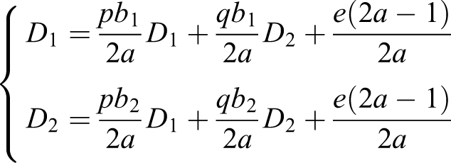
Proof. 1) Follows from lemma 2.2. 2) This equilibrium is possible iff inequality (26) is checked. According to equation (20), the equilibrium exists under equation (27). 3) Since in this case the environment is 4) According to equations (19) and (20), the equilibrium exists iff 5) Follows from lemma 2.1. 6) The system of equation (2) turns into


The solution is

It is clear that
that is


Under inequalities (30) and (31), the inner equilibrium is

Remark 3.1. The signs of the following derivatives show how a change in the types’ productivities
influences volumes of investments


Thus, with an increase in productivity of first type agents, their equilibrium investments increase if the second type consists of more than one agent (q > 1) or if q = 1 but this agent is productive and decrease if q = 1 and this agent is unproductive. The equilibrium investments of the second type agents always decrease.
With an increase in productivity of the second type agents, their equilibrium investments always increase, and the equilibrium investments of the first type agents always decrease.
Adjustment dynamics and dynamic stability of equilibria
Now, we introduce adjustment dynamics which may start after a small deviation from equilibrium or after junction of networks each of which was initially in equilibrium. We model the adjustment dynamics in the following way.
Definition 4.1
In the adjustment process, each agent maximizes her utility by choosing a level of investment; at the moment of decision-making, she considers her environment as exogenously given. Correspondingly, if

Definition 4.2
The equilibrium is called dynamically stable if, after a small deviation of one of the agents from the equilibrium, dynamics starts which returns the equilibrium back to the initial state. In the opposite case, the equilibrium is called dynamically unstable.
As before, let us consider complete network with p agents with productivity
Assume that either

with initial conditions

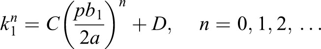
Proposition 4.1. The general solution of the system of difference equation (32) has the form

where
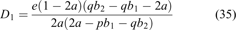

The solution of the Cauchy difference problems (32) and (33) has the form
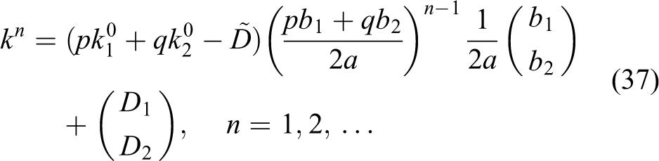
where

Proof. The characteristic equation of system (32) is

Thus, the eigenvalues are

An eigenvector corresponding

while an eigenvector corresponding

We find

The general solution of the homogeneous system of difference equations corresponding (32) has the form

As a partial solution of the system (32), we take its steady state, that is, the solution of the linear system
The solution is (35) and (36); hence, the general solution of the system (32) has the form (34). In solution of the Cauchy problems (32) and (33), constants of integration are defined from the initial conditions
However, since one of the eigenvalues is 0, we need only constant C to write the solution under

We denote

Substituting for C into equation (34), we obtain equation (37). □
Let us find conditions of dynamic stability/instability for the equilibria in complete network with two types of agents which are listed in proposition 3.1.
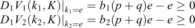
Proposition 4.2. The conditions of dynamic stability/instability of the equilibria listed in proposition 3.1 (in case of their existence) are as follows
1) The equilibrium in which both types of agents are hyperactive is stable iff

2) The equilibrium in which agents of first type are hyperactive and agents of second type are active is stable iff
3) The equilibrium in which agents of first type are hyperactive and agents of second type are passive is stable iff

4) The equilibrium in which agents of first type are active and agents of second type are passive is always unstable.
5) The equilibrium with all passive agents is always stable.
6) The equilibrium with all active agents is always unstable.
Proof.
1) According to definition 4.1 and equation (3)
Both derivatives are positive iff equation (40) is checked. 2) According to definition 4.1 and equations (3) and (27)

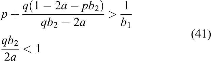
However, for dynamic stability, the strict inequality is needed. Let equation (41) be checked and

For stability, it is necessary and sufficient that 3) According to definition 4.1 and equations (3) and (28)

For stability, the strict inequalities are needed. 4) According to definition 4.1 and equations (3) and (20)
For stability, the strict inequalities are needed. Let the second inequality in equation (29) be satisfied strictly. The difference equation for any of the first group agents is

According to the first inequality in equation (29)

Hence, the equilibrium is unstable. 5) According to definition 4.1 and equation (3)
6) One of the eigenvalues of the system (32) is


Hence, the equilibrium is unstable. □
Junction of two complete networks
Let complete network 1 consists of p agents, each with productivity
Proposition 5.1
After the junction, all agents hold their initial behavior (make the same investments as before the junction) in the following four cases.
1) If 2) If
and initially agents in the first network are hyperactive and agents in the second network are passive. 3) If

and initially agents in the first network are active and agents in the second network are passive. 4) If initially agents in both networks are passive.
In all other cases, the equilibrium changes.
Proof.
1) According to corollary 2.4

Substituting
1) According to corollary 2.4

Substituting
2) Substituting

Substituting

In all other cases, the initial values of investments of agents will not be equilibrium in the unified network, and the network will move to a different equilibrium. □
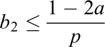
Proposition 5.1 shows, in particular, that passive agents (nonadopters), when connected with adopters, can remain nonadopters only if their productivity, b 2, is relatively low.
A pattern of transition process after the junction depends on initial conditions and parameters values. If adjustment dynamics of the unified complete network starts, it is described by the system of difference equation (32) with initial condition (33).
Proposition 5.2. Let the agents in the first network before junction be hyperactive (hence,
by corollary 2.2) and agents in the second network be passive. Then, the following cases are possible
1) If
2) If
If
In cases 2 and 3, utilities of all agents in the unified network increase. In case 1, the utilities do not change.
Proof.
Follows from proposition 5.1, point 2.
If for agents of the second group

they change their investments according to the difference equation (42). The general solution of equation (42) is
where

and

The partial solution satisfying initial conditions is
If

If
It is clear that both the equilibria

possible in result of junction are stable.
In the “resonance” case

We are looking for the partial solution of difference equation (42) not in form D, but in form

which implies

Thus, the general solution of equation (42) has the form

It follows from initial conditions that
Since

The last statement (concerning utilities) follows directly from theorem 1.2. □
Proposition 5.3
Let agents of the first network before junction be hyperactive (which implies
Proof. The first group agents stay hyperactive, because, by equation (3),

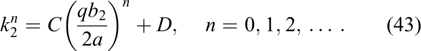
For the second group agents, we have equation (42). Its general solution is equation (43), where D is defined by equation (44). From the initial conditions, we find

Hence,
The statement concerning utilities follows directly from theorem 1.2. □
Proposition 5.4
If before junction agents of both networks are hyperactive (this implies
Proof. It follows from proposition 5.1, point 1. The increase of utilities follows from theorem 1.2. □
Proposition 5.5
If before junction agents of both networks are passive, they stay passive after junction: There is no transition dynamics, and agents’ utilities do not change.
Proof. It follows from proposition 5.1, point 4. Utilities do not change according to theorem 1.2. □
The following two propositions show how, depending on the relation between the heterogeneous productivities, passive agents (nonadopters) may change their behavior (become adopters).
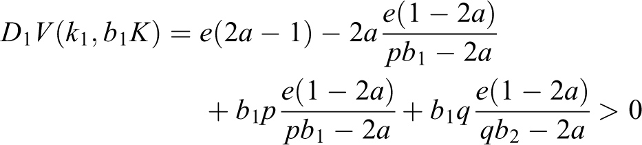
Proposition 5.6
Let agents of first network before junction be active (which implies 1) Under
Let
2) If
In case 1, utilities of all agents do not change; in case 2, utilities of all agents increase.
Proof. For the second group agents initially

Thus,
Now, let
Agents of one of the groups may achieve the investment level e earlier than the agents of another group. Let it be the first group, that is,
In the resonance case,

It follows from initial conditions that

Since
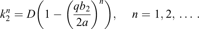
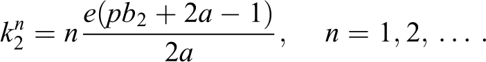
Suppose now, that the second group agents have received the investment level e first, that is,
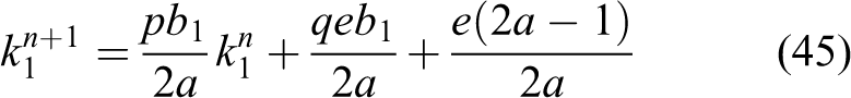
which general solution (45) is
where

From the initial condition, we have

Hence, investments of the first group agents achieve e.
In case when agents of both groups achieve investment level e simultaneously, that is,
Proposition 5.7
If before junction agents of both networks are active (this implies
Proof. The initial conditions are

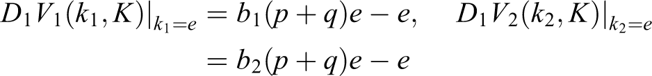
Thus, agents of both groups will increase their investments following equation (43). Agents of one of the groups will achieve investment level e first. Let it be the first group and let investments of the second group agents in this moment be

Hence,
Remark 5.1
In all cases considered in propositions 5.1–5.7, agents’ utilities in result of junction do increase or, at least do not change. Thus, all the agents have an incentive to unify, or at least have no incentive not to unify.
Remark 5.2
We have studied equilibria for complete networks formed in result of junction of two complete networks with p and q nodes. These equilibria do correspond to equilibria in some regular (equidegree) networks. For example, let
Equilibria in star network with heterogeneous agents
Analysis of equilibria with heterogeneous agents in incomplete networks is much more complex than in complete networks, because there is no common for all agents environment.
Let us consider star network with ν peripheral nodes (rays). The agent in the center of the star has productivity
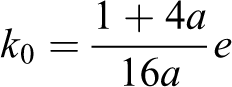
Example 6.1
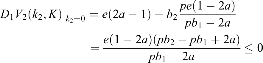
In equilibrium under

whose solution is


For the equilibrium to exist, the conditions

have to be checked. The inequality
For instance, let

that is,
Thus, in a star with six peripheral nodes, under

there exists an equilibrium in which the central agent is active and invests
One of the peripheral agents is hyperactive; two peripheral agents are active and make investments
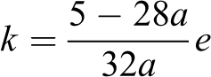
and three peripheral agents are passive.
Let us consider inner equilibrium (in which all agents are active) in star network. The investment, k, of each peripheral agent is the same (because they receive the same externality). Let us see, how the values of investments,
Theorem 6.1. For the star network, let the following inequalities be checked (if the number of peripheral nodes, ν, is sufficiently big, these three inequalities reduce to
)

Then, in the inner equilibrium 1) If

then 2) If

then 3) If

then
4)
5)

as
6)
k decreases in
7) If
8) If
9) k decreases in ν and converges to 0 as
Proof. Equilibrium investment values,
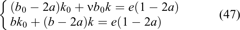
and satisfy inequalities

The solution of equation (47) is
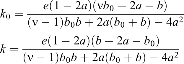
Conditions

are satisfied iff

that is

Conditions

are satisfied iff

It is defined by the sign of

that is, by the sign of

1) We obtain

Thus, 2) Differentiating

According to equation (46),
as
The value
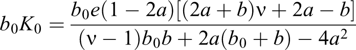
increases in ν

Hence, utility of the central agent increases if the number of peripheral agents rises. 3) We obtain

Thus, the equilibrium value k decreases in 4) We obtain

Hence, the sign of derivative is defined by the sign of the quadratic trinomial

The roots of the trinomial are

Thus, if 1) If 2) Differentiating k with respect to ν (taking ν as a continuous variable), we obtain

by equation (46). Thus, the equilibrium value k decreases in ν. It is easily seen that it converges to 0 as
The derivative of

with respect to

Thus, utility of peripheral agents decreases under growth of the star if
One important result of theorem 6.1 is that the utility of the central agent,
Tables 1 –3 summarize other results of theorem 6.1.
The dependence of investment of the central agent,

The dependence of investment of each peripheral agent, k, on parameters.

The dependence of the utility of the peripheral agent, U, on the number of peripheral agents, ν.

We see that, in the inner equilibrium, investment of any of the two counterparts, center and periphery, depends negatively on the productivity of the other counterpart. The own productivity also plays role, but in dependence of investment on the productivity of the counterpart. Investment of any agent, central or peripheral, depends positively (negatively) on the own productivity if the productivity of the counterpart is sufficiently high (sufficiently low, correspondingly).
Conclusion
Research on the role of heterogeneity of actors/agents in social and economic networks is rather new in the literature. In our model, we assume presence of two types of agents possessing different productivities. On the first stage (in time period 1), each agent in network may invest some resource (money or time) to increase her gain on the second stage (in period 2). The gain depends on her own investment and productivity as well as on investments of her neighbors in the network. Such situations are typical not only for social systems but also for various economic, political, and organizational systems. In framework of the model, we consider relations between network structure, incentives, agents’ behavior, and the equilibrium state in terms of welfare (utility) of the agents.
We prove that agent’s utility depends monotonously on her environment (the sum of her own investment and her neighbors’ investments) and provide description of agent’s behavior in terms of pure externalities and in terms of environments. We show that in inner equilibrium, the agent’s behavior is completely defined by her generalized α-centrality which depends not only on her position in the network but also on her relative productivity.
We touch some questions of network formation and identify agents potentially interested in particular ways of enlarging the network. In star network, the central agent is always interested in enlarging the networks, while the peripheral agents are interested in this only if their productivity is sufficiently low in comparison with the central agent’s productivity.
We introduce adjustment dynamics which may start after a deviation from equilibrium or after a junction of networks initially being in equilibrium.
We study behavior of agents with different productivities in two complete networks after junction. In particular, we are interested how nonadopters (passive agents) change their behavior (become adopters). If a network consisting of nonadopters (passive agents) does unify with a network consisting of adopters (active or hyperactive agents), and the nonadopters possess a low productivity, then there is no transition process, and the nonadopters stay passive. Under somewhat higher productivity, the nonadopters become adopters (come to active state), and under even higher productivity, they become hyperactive.
Agents who are initially active in equilibrium in complete network (which implies that their productivities are sufficiently high) may also increase their level of investment in result of unification with another complete network with hyperactive or active agents. The unified network comes into equilibrium in which all agents are hyperactive.
A natural task for future research is to expand the results to broader classes of networks.
Footnotes
Declaration of conflicting interests
The author(s) declared no potential conflicts of interest with respect to the research, authorship, and/or publication of this article.
Funding
The author(s) disclosed receipt of the following financial support for the research, authorship, and/or publication of this article: The research is supported by the Russian Foundation for Basic Research (project 17-06-00618).