Sage Journals: Discover world-class research

Abstract

The scale and functional complexity of future-generation wireless sensor networks will call for a non-homogeneous architecture, in which different sensors play different logical roles or functions, or have different physical capabilities in terms of energy, computing power, or network bandwidth. When sensors of the same group need to communicate with each other, their communications often have to pass through other sensors, thus forming an overlay on top of the wireless sensor network. The topology of the overlay is critical. It must have a low diameter to reduce the communication latency between those sensors. It also needs to avoid using other sensors for relaying the communications as much as possible, so as to preserve the energy of other sensors. In this paper, we propose a distributed overlay formation protocol taking account of the above factors. Through simulation, we compare our protocol with two overlay formation protocols, one that generates a fully connected topology and the other a minimum spanning tree. The results show that our protocol can achieve better performance both in message latency and energy consumption.

Keywords

Overlay Network Formation Backbone Heterogeneity

1. Introduction

As techniques and applications of wireless sensor networks mature, we expect their scale and functional complexity to increase dramatically. Progressively, they will move away from homogeneous architectures and become more and more heterogeneous [1–6]. Heterogeneity may come in different flavors. For example, different sensors in the network may have different physical capabilities, such as energy, computing power, network interface, sensing modules, and communication bandwidth. Even if sensors are homogenous physically, different sensors may play different roles and assume different responsibilities, e.g., cluster heads in a hierarchical sensor network. Sensors in a heterogeneous wireless sensor network can thus be classified into groups according to their characteristics and attributes.

Sensors of the same group may need to communicate with each other. If these sensors are scattered in different locations of the sensor network and they use the same network interface as others, then the communications between these sensors have to pass through other sensors. Logically, these sensors are interconnected by an overlay network, which is laid on top of the underlying wireless sensor network. Without loss of generality, we will call the sensors under consideration as powerful sensors and those not in the group as normal sensors.

The topology of the overlay network is critical. The overlay must have a low diameter to reduce the communication latency between the powerful sensors. It also needs to avoid using normal sensors for relaying messages as much as possible, so as to preserve the energy of normal sensors. At one extreme is a fully connected overlay, in which every powerful sensor has an overlay link to every other powerful sensor. However, since an overlay link may lay over a number of normal sensors, the more overlay links there are, the more normal sensors will be used to relay messages and consume their energy. Another extreme in the spectrum is a ring or linear list. Although a ring can minimize the number of overlay links, the communication path between any two powerful sensors may be too long to support upper-layer applications efficiently. Apparently, we need to find a middle ground to balance between application efficiency and sensor power consumption.

In this study, we first introduce three basic overlay formation mechanisms based on a centralized approach. The results then lead to our distributed overlay formation protocol. The distributed protocol aims to achieve two goals. The first is to provide efficient communications between the powerful sensors in the overlay. The second goal is to reduce the power consumption of the normal sensors for relaying messages for the powerful sensors. The protocol consists of two phases. In the first phase, powerful sensors discover some number of other powerful sensors as their neighbors. This limits the degree of a powerful sensor in the overlay. In the second phase, powerful sensors try to eliminate redundant messages and use the shortest paths for message forwarding by building a spanning tree out of each powerful sensor. This procedure is called active edge pruning (AEP). Details will be given later.

The rest of this paper is organized as follows. Section II describes our problem. In Section III, we discuss and compare three basic overlay formation mechanisms. Then we propose our distributed overlay formation protocol in Section IV. Performance evaluation of the discussed algorithms are presented in Section V. Related studies are given in Section VI. We summarize the paper in Section VII.

2. Problem Statement

Consider a sensor network G(V, E), where V represents the set of sensors ν _i for 1  ν _i  |V|. A link ν _i → ν_j ∊ E if ν _j is within the radio range of ν _i and ν _i can send a message to ν _j directly. Without loss of generality, we assume that the sensor network consists of two types of nodes: powerful and normal sensors, denoted V_PN and V_SN respectively. They are placed randomly in the field, and the number of powerful sensors is known. The communication between the powerful sensors requires the normal sensors in between to relay. The network formed by V_PN and the communication paths between them form an overlay.

An overlay over the powerful sensors may take various topologies. Different applications may prefer different overlays. In this study, we consider an overlay that interconnects all powerful nodes in V_PN and the diameter of the overlay, measured in number of hops through the normal sensors, is the minimum. That is, the problem is to

min max {p a t h l e n g t h (v_{i}, v_{j}) ∣ \forall v_{i}, v_{j} \in V_{P N}},

(1)

where pathlength(ν _i , ν _j ) is the number of hops to send a message from νv_i to ν _j . Such an overlay is useful for applications such as multicast and resource discovery in sensor networks, in which a powerful sensor needs to send a message to all other powerful sensors.

In addition to forming desirable topologies, the overlay formation protocol also needs to prolong the lifetime of the sensor network G by balancing the energy consumption of the normal sensor nodes in V_SN that help relay messages among powerful nodes. This can be expressed as follows.

max min {l i f e t i m e (v_{j}) ∣ v_{j} \in V_{S N}},

(2)

where lifetime(ν _j ) is the time interval starting from the network initialization until νv_j runs out of its energy.

In summary, the goal of our study is to design an overlay formation protocol that allows a powerful node to disseminate data to other powerful nodes efficiently. Meanwhile, the protocol should lengthen the life time of the sensor network as much as possible.

To simplify the discussion, we assume that the sensor nodes in the network have an identical radio communication range, which is modeled as a disk. The communication between two neighboring sensors is assumed to be symmetric. We also assume that wireless ad hoc end-to-end routing protocols such as AODV [7] and TORA [8] are available for routing messages between sensors. We will use the hop count to estimate the delay of sending a message from ν _i to ν _j .

Each node ν _i ∊ V has an initial energy budget denoted as EB(i). Normal sensors have a finite energy budget EB. Each node ν _i ∊ V takes E_snd and E_rcv energy units to send and receive a message, respectively. A node ν _i can send (or receive) a message if EB(i)-E_snd > 0 (or EB(i)-E_rcv > 0). A node ν _i is treated as a dead node if EB(i) = 0. After ν _i has sent (or received) a message, then EB(i) becomes EB(i) = EB(i)-E_snd (or EB(i) = EB(i)-E_rcv).

3. Centralized Approaches

In this section, we present three centralized algorithms for forming an overlay network comprised of powerful nodes. They represent different extremes in the spectrum of overlay topologies and serve as a basis for comparison with our proposed distributed algorithm, to be presented in the next section. The metrics for comparison are listed below.

Total number of messages (T_m): This is the number of messages required to disseminate a data item from a powerful node ν _i ∊ V_PN to all nodes in V_PN — {ν _i }.

Average message delay (D_m): This metric measures the average delay required to send a data from ν _i ∊ V_PN to each node V _j ∊ V_PN — {ν _i }.

Link cost (L_c): The link cost is the total number of wireless links required to maintain the connectivity of all nodes in V_PN.

Average node degree (N_d): This metric indicates the total inbound and outbound degrees of the node.

3.1. Fully Connected Overlay (FC)

Giver a sensor network G(V,E), where V = V_PN ∪ V_SN, the fully connected network (FC) is to let each V_i ∊ V_PN construct a shortest path towards each v_j ∊ V — {ν _i }. A fully connected overlay represents one extreme in overlay topologies that emphasizes on the performance of disseminating messages to all the powerful sensors.

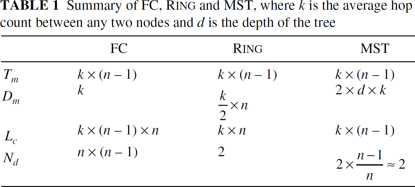
Consider a square region in which sensor nodes are randomly deployed. Suppose the network diameter is 2 × k and there are n powerful sensors. Clearly, in FC, the average number of hops of a routing path between two sensors is N_d = k. T_m is k × (n − 1) since each node in V_PN has n − 1 paths to other nodes in V_PN. The L_c in FC is k × n × (n − 1). Finally, N_d is n × (n − 1). Apparently, L_c and N_d in FC will be increased dramatically if |V_PN| increases. However, FC has the minimum D_m.

3.2 Ring-Based Overlay (Ring)

The ring-based network (Ring) formation is to construct a ring structure among nodes in V_PN. This represents another extreme in overlay topologies that emphasizes on using the minimal set of normal sensors for relaying overlay messages, whereby reducing power consumption in the normal sensors. In Ring, a node in V_PN takes a delay of $D_{m} = \frac{k}{2} \times n$ on average to send a message to another node in V_PN. T_m is kx(n − 1). N_d and L_c are 2 and k × n, respectively. Although D_m in Ring is larger than that in FC, N_d and L_c are relatively smaller.

There are different ways to building a Ring. In this study, we consider a Ring satisfying

min \sum_{v, u} message delay (v, u),

(3)

where V, u ∊ V_PN and message delay (V, u) denotes the message delay between V and u.

To solve the problem, we adopt the approximation algorithm proposed by [9]. The idea is to first build a minimum spanning tree comprised of nodes in V_PN, where the initial root node is any node in V_PN. We include the nodes and links in Ring as V_R = φ and E_R = φ, respectively. We then randomly pick a node V from the tree and include V into V_R. Starting from V, we pick a node u that has a tree link to V such that the tree link has the minimal delay among all tree links starting from V. This gives V_R = V_R ∪ {u} and $E_{R} = E_{R} \cup {\bar{v u}}$ . Node u in turn performs similar operations until V_R in Ring has the node set equal to V_PN. Possibly, u is a leaf node of the minimum spanning tree. For such a case, u performs a route towards a node w that is the successor of u in the “in-order” traversal sequence of the tree. That is, V_PN = V_PN ∪ {w} and $E_{P N} = E_{P N} \cup {\bar{u w}}$ . Node w next performs the same operations as those done by V and u.

It is proved that the ring network constructed using the above algorithm has the property that the sum of delays of sending a messages among nodes in V_PN is smaller than two times of the smallest delay.

3.3. Minimum Spanning Tree Based Overlay (MST)

It is possible to use Prime's or Krussal's algorithm to implement a minimum spanning tree (MST) on top of nodes in V_PN. If so, D_m is 2 × d × k, where d is the depth of the tree. T_m and L_c are both equal to k × (n − 1). $N_{d} = 2 \times \frac{n - 1}{n} \approx 2$ since the total in- and out-degree of nodes is 2 × (n − 1).

3.4. Comparisons

Table 1 summarizes the performance metrics of the three centralized algorithms discussed above. MST is a better choice in terms of L_c and N_d, but its D_m is larger than FC's. Ring has comparable performance as MST in terms of T_m, L_c and N_d. However, its D_m is larger than MST's, because d in MST is likely to be O(log n).

We want to note that in this section FC, Ring, and MST are centralized algorithms, which require global information to construct their overlay networks on top of V_PN. In the next section, we will introduce our proposed protocol, which is distributed without global information.

4. Proposed Protocol

In this section, our proposed overlay formation protocol is introduced. The algorithm can be divided into two parts. The first part is the basic overlay construction algorithm. In this algorithm, each powerful node tries to find a number of neighboring powerful nodes to form an overlay. We will use the term neighbor threshold to denote the number of neighbors in the following discussion.

Unfortunately, this basic construction procedure may cause redundant messages in the overlay. Thus, in the second part, we introduce a procedure called active edge pruning (AEP). This procedure builds a spanning tree over the overlay for each powerful node to eliminate redundant messages and use the shortest paths for message forwarding on the overlay.

4.1. Network Construction Algorithm

The idea of the basic overlay construction algorithm is to let each powerful node find other powerful nodes in its vicinity using expanded ring search [10]. That is, each powerful sensor A first searches other powerful sensors within its α-hop horizon (or the search range). If there exist some powerful sensors, A then records the hop distance and identifier (id in short) of those sensors. Otherwise, A expands its search to the (α + δ × k)-hop horizon, where k = 1, 2, 3, … Note that k can be chosen properly according to the network diameter.

Algorithm 1 shows the overlay initialization operation of our algorithm, where nn is the minimum number of neighbors that each overlay node will have. This value will affect the shape of the resultant overlay and can be used to control the diameter of the formed overlay. nbr[nn] _i is the buffer to store neighbor information, including node id and corresponding hop count.

Table 1
Summary of FC, Ring and MST, where k is the average hop count between any two nodes and d is the depth of the tree

FC Ring MST

T_m k × (n − 1) k × (n − 1) k × (n − 1)

D^m k $\frac{k}{2} \times n$ 2 × d × k

L_c k × (n − 1) × n k × n k × (n − 1)

N_d n × (n − 1) 2 $2 \times \frac{n - 1}{n} \approx 2$

	FC	Ring	MST
T_m	k × (n − 1)	k × (n − 1)	k × (n − 1)
D^m	k	$\frac{k}{2} \times n$	2 × d × k
L_c	k × (n − 1) × n	k × n	k × (n − 1)
N_d	n × (n − 1)	2	$2 \times \frac{n - 1}{n} \approx 2$

Lines [1–7] are the main procedure for constructing an overlay. Its task is to find a set of neighbors for each overlay node. First, line [2] uses a expended ring search (ERS) [10] to find a set of initial neighbors. In the algorithm, TRIES is used to limit search time of EPS. In line [1], a node will stop searching when it has found enough neighbors or it cannot find enough nodes after tried TRIES times. This is to prevent a far away node from flooding to the whole network.

Unfortunately, the algorithm in Algorithm 1 cannot guarantee connectivity of the overlay, because each node will stop finding neighbors if it has found enough neighbors. It is possible to form multiple disjoint overlays. With the assumption that the size of V_PN is known, each node can check the connectivity of the overlay when it builds the spanning tree. If the overlay is disconnected, a special flooding is conducted for each source. Details will be given later.

Algorithm 1

Algorithm of overlay initialization, where nn denotes the minimum number of neighbors that a node would have, nbr[nn] _i represents the set of neighbors of node i (nbr[nn] _i includes the id of each neighbor and the distance in hopcount from i to the neighbor), TRIES is the number of search times, and D_ji denotes the distance from j to i.

4.2. Active Edge Pruning

After the powerful nodes have connected to some nearby neighbors, we then build a shortest-path tree for each node. The reason is to eliminate redundant messages due to broadcasting messages in the overlay. We build a spanning tree, like a minimum cost spanning tree in Section III. This spanning tree is well suited for sensor networks because the low mobility of sensors reduces the tree maintaining cost. However, considering the routing efficiency for each node, building multiple spanning trees rooted at each node is preferable.

Thus we propose a mechanism, active edge pruning (AEP), to construct spanning trees. The idea is to choose the shorter links to the tree root and prune unnecessary links. Figure 1 shows a spanning tree rooted at node A. The solid lines are tree links and dotted lines are pruned edges. The detailed algorithm is given in Algorithm 2.

Figure 1

A spanning tree rooted at node A.

In Fig. 1, when node A wants to build its own spanning tree, namely tree A , it will broadcast a BuildTree command to the overlay. If node B receives this command from node C for the first time, B will take C as its parent in tree A and send an ACK to C . Then, C will add B as its child in tree A . If B already has a parent, it will compare the distance to A through C with its original distance to A . If the distance through C is shorter, then B will send an ACK to C and a NACK to its original parent who will remove B from its child list. B then calculates its distance to its parent and re-broadcast the command with the distance information to other neighbors. The message loop is eliminated by packet sequence. After all the powerful nodes receive the command, a spanning tree rooted at node A is formed. These steps will be conducted at every overlay node to construct their own spanning tree.

Algorithm 2

Algorithm of active edge pruning, where C M D_BT denotes the command—BuildTree—that is originated from source S, DIST_SJ represents the distance from source S to itself through neighbor J in hops, and DIST_Scur denotes the currently shortest hopcount from source S to itself in hops.

This tree building process can also help to repair the tree on node failure. Each tree root will collect information of all tree members in the tree building process. When the root could not receive responses from a certain node, it will try to repair the tree by finding a direct route to that node. This could guarantee the integrity of each tree and connect each overlay partition.

4.3. Overlay Maintenance

When the system runs for some time, the relaying nodes on the overlay links will run out of their energy, thereby breaking the links. There are at least two strategies to maintain an overlay. First, when an overlay node finds that its relaying neighbor fails, the overlay node had to find another link to keep the connectivity of the overlay. Second, the overlay could notify the nodes to change their links. The former can be done by simply selecting new neighbors from the candidate set collected from overlay initialization as mentioned previously. The second approach can solve the hot spot problem effectively. A hot spot is a node where a considerable amount of traffic passes through in a short period. This will cause the links nearby the hot spot to exhaust energy quickly.

Figure 2 shows two examples such that A may become a hot spot. In

when A checks its traffic history, it finds that B sends messages frequently to node X, Y , and Z through A .

is the opposite of (i), in which node A will find large amount of traffic passing from nodes B, C, D to X . In both cases, the energy of relaying nodes near A will be drained rapidly.

Figure 2

Two examples show that A may become a hot spot, where (i) shows that node B addresses a message to nodes X, Y , and Z , and (ii) shows B, C, D send messages to X .

Consider the problem in (i) first. When A observes that it receives many packets from a sender to several destinations in a short period, it will notify its upstream node M , i.e., the node which forwards the packets to it, to distribute the destinations by choosing another “lightly loaded” neighbor as the downstream node. If all neighbors of M are overloaded, M will choose the lightest among them. Similarly, the problem in (ii) can be solved by distributing the sources (i.e., nodes B, C , and D ).

5. Performance Evaluation

In this section, we will evaluate the performance of the discussed algorithms using simulations.

5.1. Experimental Settings

The evaluation is based on the ns2 simulator with the CMU wireless extension [11]. All the sensors in simulations are stationary, which are deployed uniformly at random in a square field ranging from 600m × 600m to 1000m × 1000m, subject to the condition that the network is connected. In the simulations, there are |V| = |V_SN ∪ V_PN| ≍ 130 nodes deployed in the field. We assume that each sensor has a radio range of 100m.

Each node in VSN has an initial energy budget 10 joule, and the nodes in V_PN have an infinite energy budget. We adopt the energy consumption model in [12]. A sensor node takes 81 mW to send a message and 30 mW to receive a message. The size of each simulated message is 128 bytes. We measure the remaining energy budget EB(i) of each node ν _i ∊ V_SN. Since we are interested in the performance of the overlay using different network formation algorithms, each node in V_PN will generate a message every t seconds, where t follows the exponential distribution. The default routing protocol is AODV [7]. Table 2 summarizes the parameters used in the simulations.

The performance metrics include the average message delay (D_m) of transmitting a message between any two nodes in V_PN, and the average number of messages (T_m) of disseminating a data item issued by V ∊ V_PN to nodes V_PN — {V}. We measured the remaining energy of sensor nodes in V_SN, and calculated that the CDF CDF allows us to evaluate whether the energy that remained in the different nodes was balanced or not.

Table 2
Experimental settings

Parameter Value

Network Size 600m × 600m ∼1000m × 1000m

|V| 130 ∼ 137

$\frac{∣ V_{S N} ∣}{∣ V_{P N} ∣}$ 7 ∼ 12

Radio range 100m

Traffic Exponential

Power to send a packet 81 mW

Power to receive a packet 30 mW

Energy per node in V_SN 10 joule

Packet size 128 bytes

Routing protocol AODV

Parameter	Value
Network Size	600m × 600m ∼1000m × 1000m
\|V\|	130 ∼ 137
$\frac{∣ V_{S N} ∣}{∣ V_{P N} ∣}$	7 ∼ 12
Radio range	100m
Traffic	Exponential
Power to send a packet	81 mW
Power to receive a packet	30 mW
Energy per node in V_SN	10 joule
Packet size	128 bytes
Routing protocol	AODV

5.2. Comparison of Centralized Algorithms

We first compare the three centralized algorithms discussed in Section III. The first experiment is to evaluate the effects of the size of the network. In this experiment, we let |V_PN| = 10 and $| \frac{V_{S N}}{V_{P N}} | = 8$ . Therefore, |V| = 90. The size of the simulated network region is from 400m × 400m to 800m × 800m.

Figure 3(a) depicts the simulation result of the average message delay versus the size of the network. Clearly, FC outperforms Ring and MST. MST has the message delay close to FC's. The result conforms to the performance analysis in Section III.

Figure 3

Effects of network size, where (a) the average message delay and (b) the average number of messages.

Figure 3(b) shows the result for the average number of messages required to disseminate a data item to each node in V_PN. We can see that MST takes a smaller number of messages to disseminate compared to FC and Ring. FC takes more messages to send a data item. This is because nodes in V_PN need to construct |V_PN| × (|V_PN| − 1) communication paths. When nodes in V_PN need to disseminate a data item to others, their packets may be congested, leading to retransmission of the packets. In contrast, Ring and MST use |V_PN| − 1 paths, resulting in fewer messages used to disseminate a data item.

Next, we consider the effects of |V_PN| and $\frac{| V_{S N} |}{| V_{P N} |}$ . In this experiment, $\frac{| V_{S N} |}{| V_{P N} |} = 4$ and each node has 1.5 neighbors in average. We varied V_PN from 5 to 20. Figure 4(a) shows the average message delay versus |V_PN|. The result indicates that the message delay in Ring increases dramatically, compared to FC and MST. The result conforms to our previous performance analysis. We also vary $\frac{| V_{S N} |}{| V_{P N} |} = 4$ from 4 to 9. The results are similar, and are shown in Fig. 5 .

Figure 4

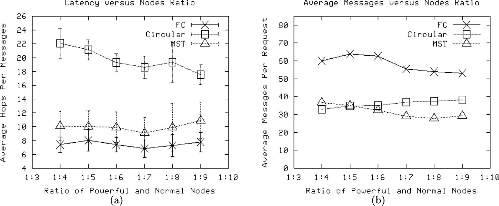
Effects of numbers of powerful nodes for $\frac{| V_{S N} |}{| V_{P N} |} = 4$ , where (a) the average message delay and (b) the average number of messages.

Figure 5

Effects of numbers of powerful nodes for $4 \leq \frac{| V_{S N} |}{| V_{P N} |} \leq 9$ , where (a) the average message delay, and (b) the average number of messages.

From the above discussion, we conclude that FC outperforms Ring and MST in terms of average message delay at the expense of creating more communication paths among nodes in V_PN. In contrast, MST outperforms FC, which takes the least number of messages to disseminate a data item. MST can prolong the lifetime of sensor nodes in V_SN.

5.3. Performance of our Proposed Algorithm

We compare FC, MST and our proposed algorithm. The number of overlay nodes is 15, and the performance for the network size from 600m × 600m to 1000m × 1000m is investigated. In this experiment, we let nn = 2, α = 3, and δ = 2.

Figure 6(a) shows the measured message latency. Our proposed protocol is better than MST and worse than FC. In Fig. 6 (b), the message cost in our protocol is obviously less than FC's and is slightly more than MST's.

Figure 6

Comparison of FC, MST, and our proposed protocol, where (a) message latency versus network size, (b) message cost versus network size, and (c) CDF of remaining energy.

The results conclude that our protocol can have a smaller message delay while keeping the message cost low. Figure 6(c) depicts the CDF for remaining energy. FC uses more energy than our protocol and MST. Our protocol is slightly better than MST.

After comparing with other protocols, we examine our proposed protocol under different settings. We first vary the number of neighbors (i.e., the neighbor threshold) that a node can have. Figure 7(a) shows that when the neighbor threshold increases, the resultant overlay could have a shorter message latency. In Fig. 7 (b), the message cost increases along with the increase of neighbor threshold. The remaining energy of nodes in V_SN increases when neighbor threshold is small, however (see Fig. 7 (c)). This is because the resultant overlay will be degenerated to FC if nn is larger. If nn = |V_PN − 1|, nodes in the overlay will be fully connected.

Figure 7

Performance of our porposed algorithm, where (a) message latency versus overlay size, (b) messages cost versus overlay size, and (c) CDF of remaining energy.

Our simulation study also varies α and δ. The simulations results are depicted in Fig. 8 (a)–Fig. 8(c). We can see in Fig. 8 (a) that a shorter search range can shorten the search delay. However, smaller α leads to the partition of the overlay network. We solve this partition problem by having each tree root build a direct route to the nodes that it did not receive a response from earlier.

Figure 8

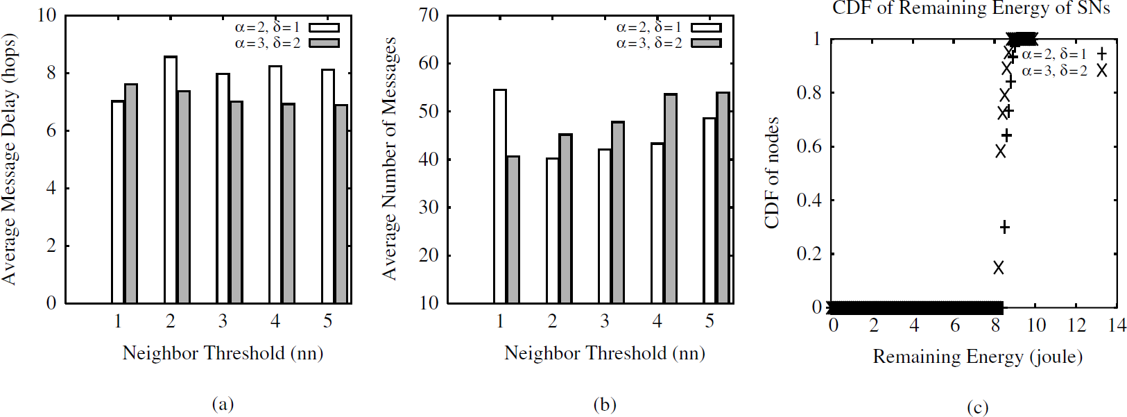
(a) Message latency versus neighbor threshold, (b) Messages cost versus neighbor threshold, (c) CDF of remaining energy in V_SN versus neighbor threshold.

From the experimental results presented in this section, we conclude that our proposal has a shorter message latency than MST's (and Ring's), and approximates to FC. Our solution outperforms FC in terms of the message cost and the CDF for the remaining energy.

6. Related Works

Various approaches have been proposed to address the power and latency problem in wireless sensor networks. Generally, they can be classified into the following categories.

Clustering: Building a layered structure by clustering sensors can both conserve energy and improve system throughput. In LEACH [13], homogeneous sensors are organized into clusters. Heinzelman et al. [5] considers a heterogeneous network composed of powerful and normal sensors. They investigate the optimal number of clusters and suitable energy allocation for each type of sensors in a heterogeneous environment to prolong the network life.

Centralized Approach: Youssef et al. [14] focus on energy conserving routing and try to maintain good routing delay in a cluster. They assume that sensors can tune the radio amplifier to change their maximum transmission range. A constrained shortest path routing protocol is proposed to adjust the radio transmission power to obtain diverse in-cluster topologies. The path to the cluster-head is then set with the minimum transmission energy. Lifetime optimization for in-home heterogeneous sensor networks is discussed in [1]. Its resource oriented protocol (ROP) divides the sensors into several energy levels. The protocol then constructs a hierarchical structure and calculates the energy-optimal topology in a centralized manner.

Dominating Set: Guo et al. [15] build a backbone-like structure using the dominating set to eliminate redundant messages during broadcast and to avoid message collision. The node receiving a broadcast packet will wait a period before it declares itself as a forwarding node. This latency is determined by the remaining power of the node.

The system model used in [5], [13] is different from ours. In LEACH [13], it assumes a homogeneous network consisting of a single base station aggregating data from a large sensing field and sensors having the capability to control radio electronics. The network model in our study is similar to [5], but [5] assumes that those overlay sensors would take turns to become cluster-heads and cover the whole area. Besides, [5] centers on finding the optimal number of clusters. ROP [1] targets at home-scale networks and periodically builds energy efficient topology for routing. Unfortunately, it is a centralized method and is not suitable for large outdoor applications.

Both dominating set [6], [15] and forwarding set selection [16] can be used to reduce redundant packets caused by the broadcast. However, our work is to provide an energy-efficient communication substrate where many applications can be implemented. Our focus is on shortening the end-to-end delay among the overlay sensors under the energy constraint of the normal sensors. Our model is established on a heterogeneous environment. These features are different from previous works.

7. Summary

In this paper, we study different overlay formation protocols through mathematical analysis and simulations. A fully connected overlay can be treated as a tree whose height is one. On the other hand, the height of a ring overlay is equal to n/2, where n is the number of overlay nodes. We then propose a novel distributed overlay formation protocol for shortening routing delay while conserving energy. Our protocol builds a spanning tree for each overlay node. These spanning trees not only are helpful for removing routing loops, but also can provide short routing paths.

Simulation results show that our protocol can achieve shorter message latency while retaining low energy deviation. We also evaluate our protocol with various parameters and the results show that by choosing a suitable neighbor threshold and search range, it is possible to obtain better performance and avoid the risk of network partition.

There are several possible improvements to our protocol. For example, we can build a layered overlay. That is, we cluster all nearby overlay nodes first and then use our protocol to build a spanning tree in each layer. Constructing such a hierarchical structure could not only save the energy consumption but make our protocol more scalable. Another possible improvement is the routing protocol of the underlay network. In this paper we only focus on solving problems on overlay, but the underlay routing deserves further study.

Footnotes

Acknowledgment

This work was supported in part by the National Science Council, R.O.C., under Grant NSC 93-2752-E-007-004-PAE, by the MOEA Research Project under Grant No. 94-EC-17-A-04-S1-044, and by the CCL of ITRI.

References

Aylor

J. H.

, “System lifetime optimization for heterogeneous sensor networks with a hub-spoke technology,” IEEE Transaction on Mobile Computing, vol. 3, no. 3, pp. 286–294, July 2004.

Mhatre

Rosenberg

, “Homogeneous vs heterogeneous clustered sensor networks: a comparative study,” in Proceedings of IEEE International Conference on Communications. IEEE Communication Society, June 2004, pp. 3646–3651.

Mhatre

V. P.

Rosenberg

Kofman

Mazumdar

Shroff

, “A minimum cost heterogeneous sensor network with a lifetime constraint,” IEEE Transaction of Mobile Computing, vol. 4, no. 1, pp. 4–15, Jan. 2005.

Singh

Prasanna

V. K.

, “A hierarchical model for distributed collaborative computation in wireless sensor networks,” in Proceedings of International Parallel and Distributed Processing Symposium. IEEE Computer Society, Apr. 2003.

Duarte-Melo

E. J.

Albert

, “Analysis of energy consumption and lifetime of heterogeneous wireless sensor networks,” in Proceedings of IEEE Global Telecommunications Conference. IEEE Communication Society, 2002, pp. 21–25.

, “On calculating connected dominating set for efficient routing,” in Proceedings of the Third International Workshop on Discrete Algorithms and Methods for Mobile Computing and Communications. ACM, Aug. 1999, pp. 7–14.

Perkins

C. E.

Royer

E. M.

, “Ad-hoc on-demand distance vector routing,” in Proceedings of Second IEEE Workshop on Mobile Computing Systems and Applications, Feb. 1999, pp. 90–100.

Park

V. D.

Corson

M. S.

, “A highly adaptive distributed routing algorithm for mobile wireless networks,” in Proceedings of INFOCOM. IEEE Communication Society, Apr. 1997, pp. 1405–1413.

Neapolitan

Naimipour

, Foundations of Algorithms, using C+ pseudocode. Jones and Bartlett, 1998, ch. Computational Complexity and Intractability: An Introduction to the Theory of NP.

10.

Hassan

Jha

, “Optimising expanding ring search for multi-hop wireless networks,” in Proceedings of IEEE Global Telecommunications Conference. IEEE Communication Society, Dec. 2004, pp. 1061–1065.

11.

ns2, http://www.isi.edu/nsnam/ns/.

12.

Miller

M. J.

Vaidya

N. H.

, “Minimizing energy consumption in sensor network using a wakeup radio,” in Proceedings of IEEE Wireless Communications and Networking Conference. IEEE Communication Society, Mar. 2004, pp. 2335–2340.

13.

Heinzelman

W. R.

Chandrakasan

Balakrishnan

, “Energy-efficient communication protocol for wireless microsensor networks,” in Proceedings of the 33rd Annual Hawaii International Conference on System Sciences, Jan. 2000.

14.

Youssef

M. A.

Younis

M. F.

Arisha

K. A.

, “A constrained shortest-path energy-aware routing algorithm for wireless sensor networks,” in Proceedings of Wireless Communications and Networking Conference. IEEE Communication Society, Mar. 2002, pp. 794–799.

15.

Guo

, “Broadcasting for network lifetime maximization in wireless sensor network,” in Proceedings of First Annual IEEE Communications Society Conference on Sensor and Ad Hoc Communications and Networks. IEEE Computer Society, Oct. 2004, pp. 352–358.

16.

Sinha

Sivakumar

Bharghava

, “Cedar: a core-extraction distributed ad hoc routing algorithm,” IEEE Journal on Selected Areas in Communications, vol. 17, no. 8, pp. 1454–1465, Aug. 1999.