Sage Journals: Discover world-class research

Abstract

Small unmanned aerial vehicles (SUAVs) are suitable for many low-altitude operations in urban environments due to their manoeuvrability; however, their flight performance is limited by their on-board energy storage and their ability to cope with high levels of turbulence. Birds exploit the atmospheric boundary layer in urban environments, reducing their energetic flight costs by using orographic lift generated by buildings. This behaviour could be mimicked by fixed-wing SUAVs to overcome their energy limitations if flight control can be maintained in the increased turbulence present in these conditions. Here, the control effort required and energetic benefits for a SUAV flying parallel to buildings whilst using orographic lift was investigated. A flight dynamics and control model was developed for a powered SUAV and used to simulate flight control performance in different turbulent wind conditions. It was found that the control effort required decreased with increasing altitude and that the mean throttle required increased with greater radial distance to the buildings. However, the simulations showed that flying close to the buildings in strong wind speeds increased the risk of collision. Overall, the results suggested that a strategy of flying directly over the front corner of the buildings appears to minimise the control effort required for a given level of orographic lift, a strategy that mirrors the behaviour of gulls in high wind speeds.

Keywords

Orographic lift fixed-wing flight control simulation SUAV

Introduction

The high manoeuvrability of small unmanned aerial vehicles (SUAVs) makes them particularly suitable for many low-altitude operations in urban environments. They have application in many different fields¹ such as border control, search and rescue, surveillance,^2–5 medical supply or parcel delivery^6,7 and natural disaster response.^8,9 Limited on-board energy^10,11 and the effect of the atmospheric turbulence at low altitudes^12–15 are two challenges that have a major effect on the flight performance of SUAVs.

On-board energy storage is limited due to the size and weight constraints of SUAVs. Batteries can constitute up to 40% of the vehicle’s mass, giving a nominal flight time of approximately 60 min for small fixed-wing vehicles.^10,11,16 This restricts the endurance and range of these aircraft, which may compromise their missions. Therefore, energy management constitutes an important challenge in the design of these vehicles.

SUAVs typically operate at low altitude in the atmospheric boundary layer (ABL). The challenge of this resides in the increase in turbulence intensity closer to the ground, where the flow is dominated by horizontal transport of atmospheric properties and wind speeds increase because of the pressure gradients caused by buildings and obstacles.¹³ This can result in wind disturbances that are the same order of magnitude as the vehicle’s flight speed. As the flight of these vehicles is characterised by low Reynolds number, low inertia, low flight speed and low stability,¹⁷ this creates a substantial challenge for flight control in some conditions.

One method for reducing the energetic cost of flight is to make use of environmental wind flows. When wind is deflected upwards by the presence of obstacles, such as hills or buildings, this creates opportunities for orographic soaring, where the sink rate of the aircraft is offset by the vertical motion of the air. Langelaan et al.¹⁸ designed a path planner for UAVs which could make use of orographic soaring through optimising a particular cost function based on knowledge of the wind field. Simulations were conducted for two unmanned aircraft, showing improvements for both optimal minimum time and optimal maximum energy trajectories compared to a constant speed trajectories. White et al.¹⁹ studied the feasibility of SUAV soaring in urban environments based on wind-tunnel experiments with scaled model buildings. The aim of this testing was to measure the relationship between the vertical component of the wind and the oncoming mean wind speeds, showing values between 15 and 50%. A further study²⁰ measured the sink rate of a soaring MAV and concluded that depending on the wind strength and direction, it is feasible for a MAV to exploit orographic soaring next to buildings. A MAV platform and control system was later designed to try to mimic the kestrel’s ‘wind-hovering’ strategy, holding the MAV’s longitudinal and lateral position.²¹ Flight tests were conducted around two locations: a hill and a building. The former resulted in consistently successful soaring flights while tests around the latter could not be sustained for over 20 s, which was attributed to gustiness. A CFD model to simulate the turbulent wind flow conditions surrounding buildings was designed by Mohamed et al.,²² with the aim of providing the potential energy available for harvesting. This model was used to locate suitable areas of lift, which were then tested in flight trials.²³

Birds fly in the same conditions as SUAVs and face similar challenges in energy management and flight control. Birds frequently reduce their energy expenditure by exploiting environmental wind fields such as tailwinds, wind gradients and updraughts. Of particular interest for SUAV flight control is how birds exploit orographic updraughts generated by man-made structures, with birds being observed soaring on the upwind side of ferries²⁴ and buildings.²⁵ Shepard et al.²⁵ studied gulls exploiting orographic updraughts by soaring parallel to the face of buildings. The two main findings of this work were that birds used the updraughts to maintain height rather than to gain it and that they positioned themselves in specific regions of the wind field depending on the strength of the wind. It was hypothesised that the gulls flight control requirements in gusty conditions were reduced in these specific regions of the wind field.

Following the work from Shepard et al.,²⁵ the aim of this study is to investigate the control requirements for a powered SUAV to take advantage of orographic soaring when flying along a row of buildings. This is done by simulating an SUAV holding position relative to buildings whilst flying through different wind fields measured in Shepard et al.²⁵ Control effort (CE) is used to compare the control demand of different simulations and ultimately of flights in different regions of the wind field. First, a flight guidance, navigation and control (GNC) framework is described in ‘Framework’. The specific atmospheric conditions, a description of the SUAV and an overall view of the metrics and simulations used are then given in the ‘Simulations’ section. Results are shown and discussed in the ‘Results and discussion’ section and conclusions are drawn in the ‘Conclusions’ section.

Framework

Simulations were carried out using a 6 DOF flight GNC framework implemented in Simulink (MathWorks, MA, USA). This model was used to simulate the behaviour of a powered SUAV flying in gusty, windy conditions.

Guidance

The flight guidance system calculated the changes in pitch and yaw angle required to follow a predefined trajectory based on the SUAVs inertial position.

Altitude control – pitch angle desired

Altitude was controlled by means of a pitch controller adjusting the elevator. The desired pitch angle was calculated following the block diagram in Figure 1.

Lateral control – yaw angle desired

Figure 1.

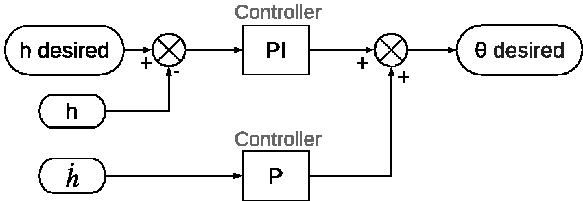
Altitude controller block diagram. h is the altitude, $\dot{h}$ is the vertical speed and θ is the pitch angle of the aircraft.

The lateral position was controlled by means of the ailerons and rudder. The desired yaw angle required to follow the path was calculated following the block diagram in Figure 2.

Figure 2.

Lateral position controller block diagram: χ is the course angle, y is the lateral position of the vehicle and ψ is the yaw angle of the aircraft.

The course angle was defined as the angle between North and the direction of movement of the vehicle. The desired course angle was obtained by looking at a point in the trajectory which was at a distance L1 from the vehicle. L1 was set as 25 m in this study. Under no wind perturbations, the course angle is equal to the heading angle (yaw angle). However, to counteract the wind effects, a PI controller was used with the lateral position error to correct the drift caused by the wind.

Navigation

Following the work of Langelaan et al.²⁶ and Depenbusch,²⁷ the 6DOF flight dynamics equations used in this work are presented in Appendix 1. Figures 3 and 4 show the general structure used to model the flight dynamics.

x and u are the state and control vectors defined in equations (1) and (2) below. V_a is the airspeed, α is the angle of attack, β is the sideslip angle, [p, q, r] are the roll, pitch and yaw body rotation rates, respectively, and [ $ϕ$ , θ, ψ] are the corresponding Euler angles. δ_i for i = ail, ele, rdd and thr is the deflection angle of the aileron, elevator and rudder and the commanded value of throttle, respectively

x = [V_{a}, α, β, p, q, r, ϕ, θ, ψ]

(1)

u = [δ_{ail}, δ_{ele}, δ_{rdd}, δ_{thr}]

(2)

[x, y, z] represented the position of the aircraft expressed in the inertial NED reference system fixed to the ground.

Figure 3.

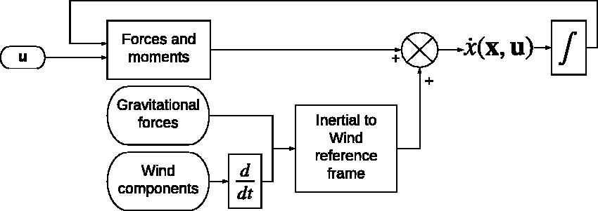
Block diagram of the flight dynamics equations.

Figure 4.

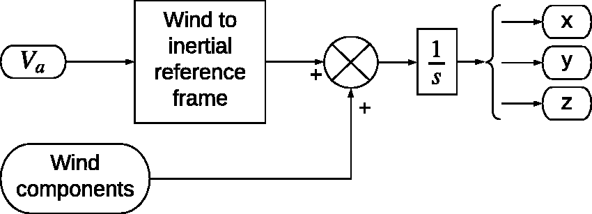
Block diagram of the inertial position of the aircraft.

Control

The flight control framework was composed of a series of controllers which allowed the aircraft to keep steady-level flight and hold its lateral position. Block diagrams of the controllers are presented in Figures 5 to 7. These controllers were designed as follows.²⁸

Figure 5.

Pitch controller block diagram.

Figure 6.

Airspeed controller block diagram.

Figure 7.

Course controller block diagram.

Note that U₀ is the equilibrium airspeed in stability axes and $τ_{ψ}$ and τ_r are time constants.

Limitations

The model did not account for some of the physical limits of the aircraft or the environment. Phenomena such as stall and ground effect were not taken into account. The aircraft was modelled as a point mass, with the distribution of the wind across the wing span not being considered in the flight dynamics of the aircraft.

Simulations

The ultimate goal of this work was to study the control costs of a SUAV when soaring close to buildings, determining if there was a benefit to flying in particular regions of the wind field. This was investigated by simulating a SUAV flying close to a simulated row of buildings in a range of different wind conditions. The aircraft’s controllers were set to hold airspeed, height and lateral position. In particular, the desired airspeed was kept constant and equal to 12.7 ms^(-1) throughout the simulations, and the 26 combinations of desired height and lateral positions studied are defined in Figure 8.

Figure 8.

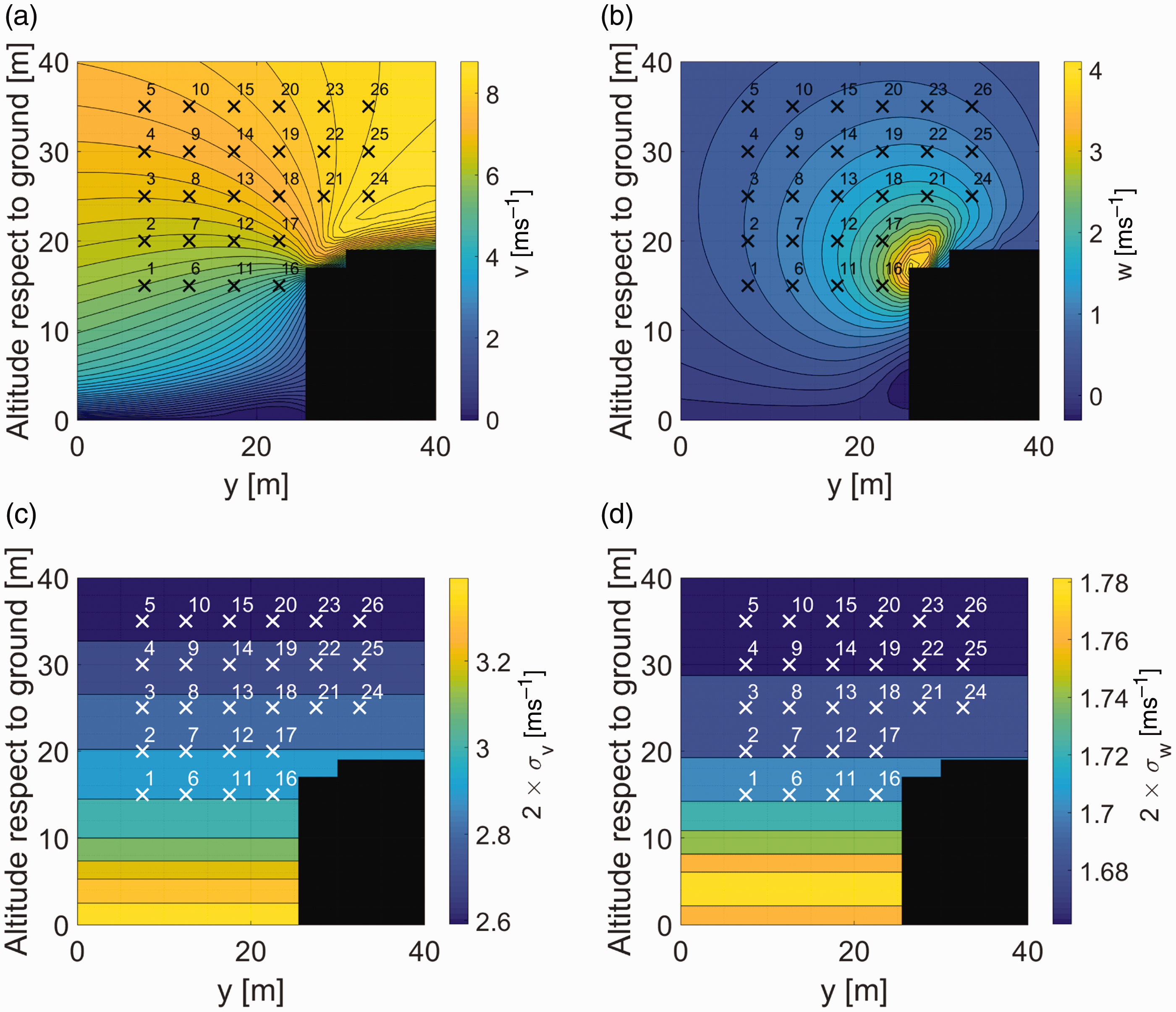
Contour plots of lateral (v) and vertical (w) components of the wind together with the imposed vertical and lateral positions studied (‘x’ symbols) for W20 = 9.34 ms^(-1). 8(a) and 8(b) give the distribution of v and w wind vector components. 8(c) and 8(d) show the distribution of the v and w wind vector components of the Dryden disturbance model. These are given as $2 \times σ_{v}$ and $2 \times σ_{w}$ respectively, corresponding to 95% confidence interval range for the change in wind speed. The strength of the wind components is illustrated with the colour scale, with a resolution of 0.2 ms^(-1) between contour levels for Figures 8(a) and (b); and a resolution of 0.1 ms^(-1) for Figure 8(c) and 0.02 ms^(-1) for Figure 8(d).

Wind field

The urban wind field used in this study was generated by Shepard et al.²⁵ for periods of onshore winds in Swansea Bay, UK. Here, the wind came in over the open sea before meeting a row of four-storied buildings, which deflected the air upwards causing orographic lift. Shepard et al.²⁵ found that the total number of gulls observed soaring by the sea-front in this area increased with wind strength and varied with wind direction. There was a peak in the total number of birds observed for winds from around 150° (SE), which coincided with the wind being perpendicular to the front face of the buildings.

The wind field data were simplified for the simulations by averaging along the direction of flight. This simplification allowed the simulation to run indefinitely, modelling the SUAV flying parallel to a long row of buildings. The two wind fields used in this study had considerably different nominal wind speeds at 20 ft (W20), W20 = 2.26 ms^(-1) and W20 = 9.34 ms^(-1), but similar wind directions, 140.8° and 137°, respectively. Figures 8(a) and 8(b) show a cross-section of one of the wind fields used along with the desired SUAV positions tested.

The Dryden model was used to add a continuous level of disturbance to the steady-state wind field already described. This mathematical model representing the frequency spectrum of continuous gusts was integrated into the flight dynamics equations of motion as an atmospheric disturbance. In this work, the MIL-F-8785C²⁹ specification was applied through the ‘Dryden Wind Turbulence Model (Continuous)’ block in Simulink for low-altitude applications. This model provides both translational and rotational disturbance velocity components. In this particular case, a comparative study using both the translational and rotational components, and the translational components only showed no major difference in the results obtained. Therefore, only the translational components were used for this work. The input required in each simulation was the nominal wind speed at 20 ft (W20) and the wind angle with respect to North. The equations defining the model can be found in Appendix 2. Three low-altitude disturbance levels were studied, defined as: WFDi with i = 75, 100 and 125% of W20 = 2.26 ms⁻¹ and W20 = 9.34 ms^(-1). Figures 8(c) and (d) show the variation of the wind field due to the Dryden disturbance model on its own. The Dryden model does not take into consideration the natural or artificial obstacles in the environment. Because of that, the disturbance level and standard deviation are only affected by the vertical distance from the ground. The standard deviation of the disturbance added by the Dryden model reaches values of up to 20% of W20 for u and v, and up to 10% of W20 for w.

Control effort

In this work, CE refers to the amount of control necessary to keep steady-level-flight whilst holding a specific lateral and vertical position parallel to the buildings. This term is used as a parameter to compare the control demand of different simulations and ultimately of flights in different regions of the wind field.

Considering the rate of change in the control surface deflection and in the throttle demand as a measurement of how much these are being used to control the vehicle, equations (3) to (5) define the CE parameter used in this study.

The deflection angle for the three control surfaces and the demanded throttle value is normalised by their maximum achievable value. Deflection limits are gathered in Appendix 3

δ_{i_{norm}} = \frac{| δ_{i} |}{\max {δ}}

(3)

δ_{i_{rate}} = \frac{d}{d t} δ_{i_{norm}}

(4)

The deflection rate is defined as a timeseries and its root-mean-square (RMS) is reported here

C E_{i} = RMS (δ_{i_{rate}}) = \sqrt{\frac{1}{n} \sum_{i = 1}^{n} δ_{i_{rate}}^{2}}

(5)

SUAV platform

A non-linear flight dynamics model of an instrumented WOT 4 Foam-E Mk2+ (Ripmax, Enfield, UK) (Figure 9) has been derived from outdoor flight tests using the output error method and has been integrated in the model. This vehicle is 1.345 kg and has a 1.205 m span with an aspect ratio of 4.85. It has three control surfaces: elevator, rudder and ailerons.

Figure 9.

Ripmax WOT 4 Mk 2 UAV.

The servo motors and the electric engine responses have been simplified and defined as a linear second-order transfer function

G (s) = \frac{ω_{n}^{2}}{s^{2} + 2 ζ ω_{n} s + ω_{n}^{2}}

(6)

The main physical and aerodynamic characteristics of this platform, the control PID gains for each one of the controllers and the natural frequency ( $ω_{n}$ ) and damping ratio (ζ) of the transfer functions are given in Appendix 3.

Results and discussion

In this section, results are presented for the different atmospheric effects described in ‘Simulations’. Flights under these conditions were simulated for a desired airspeed of 12.7 ms^(-1), and for 26 different paths.

The results showed that the CE required to maintain steady-level-flight and lateral position strongly depended on the height at which the SUAV was flying. Figure 10 shows the trend of this parameter for the three control surfaces and the commanded throttle. The CE with respect to the imposed height is presented for the six different atmospheric conditions studied. The CE required decreased as the imposed height increased for all control surfaces and the throttle in all wind conditions. The slight difference in the pattern shown for the elevator for the most turbulent wind field (WFD125 9.34) was due to the aircraft crashing for some paths close to the buildings. There are two factors that could have an important role in the explanation of this trend. First, the disturbance intensity was correlated with the inverse of the height (Figures 8(c) and (d)), and more CE is required at higher disturbance intensities. Second, the mean wind fields close to the buildings had a greater horizontal variation at lower heights (Figures 8(a) and (b)), which would also have increased the wind gradient experienced by the UAV if it moved laterally. Figure 10 also shows that as the wind speed increased (W20), the CE required also increased. This was as expected because the disturbance intensities of the Dryden model are proportional to the mean wind speed.

Figure 10.

Control effort pattern for the control surface and throttle command versus the imposed flight height for six different atmospheric conditions: WFDi for i = 75, 100 and 125 is the wind field with the Dryden noise, i being the percentage of W20 used for the simulation. Dashed lines represent the data for W20 = 2.26 ms^(-1) and solid lines, W20 = 9.34 ms^(-1). The mean CE value at each imposed height is shown in these figures. Figures 10(a) and (c) on the left-hand side show the effects in the longitudinal dynamics while Figures 10(b) and (d) present the patterns in the lateral dynamics.

Comparing two points in the wind field at the same radial distance to the buildings, Shepard et al.²⁵ suggested that the birds’ flight control requirements may be reduced at higher angle positions than at lower angles. It is important to highlight the fact that as the angle decreases for a constant radial distance, so does the height. Their hypothesis was that at higher angles, birds find a position with a greater velocity stability: lateral displacements do not have a strong effect because they remain in the same contour level and vertical displacements could appear to be self-stabilising. The results shown in Figure 10 are consistent with this hypothesis.

The CE definition used in this work takes into consideration the rate of change of the control surfaces and throttle input. This parameter allows for different paths and wind fields to be compared from a control point of view. However, it is important to note that the throttle value at which the SUAV is flying is also an important factor in the energy consumption of the vehicle and hence, a meaningful parameter to consider to improve SUAV flight performance. Unlike the CE trends, the mean throttle value shows a strong dependency with the radial distance to the buildings. This trend indicates that there is an effect caused by the orographic lift (Figure 8(b)). Figure 11 shows this trend for the six different wind conditions studied. These curves have been obtained by curve fitting the data from the successful paths: where the SUAV has not crashed against the ground or the buildings during simulation. Because of this, the data points used to fit the curves in the case of W20 = 9.34 ms^(-1) are limited in close proximity to the buildings. Note that the throttle command is defined in the limits [0, 1]. The curves in this figure suggest that the SUAV required less throttle input; the stronger the wind field and the closer it was to the buildings. For the slower mean wind speed, the level of disturbance had no significant effect on the mean throttle, but for the stronger wind field, a greater level of disturbance correlated with a lower mean throttle. However, as shown in Figure 12, for the faster wind field, the closer the SUAV path was to the buildings the greater the risk of collision with increased levels of turbulence, with positions 16 and 17 crashing for WFD75 of 9.34 ms^(-1), positions 12, 16 and 17 for WFD100 and positions 11, 12, 16, 17 and 21 crashing for WFD125. These failed flights indicate the risk of flying close to the buildings under strong wind conditions.

Figure 11.

Mean throttle value respect to the radial distance to the buildings for six different atmospheric conditions: WFDi for i = 75, 100, 125 is the wind field with the Dryden noise, i being the percentage of W20 used for the simulation. Dashed lines represent the data for W20 = 2.26 ms⁻¹ and solid lines, W20 = 9.34 ms⁻¹.

Figure 12.

Contour plots of lateral and vertical components of the wind for W20 = 9.34 ms⁻¹ with the imposed vertical and lateral positions studied (‘x’ symbols), and the red circles symbolise the flights that crashed against the ground or the buildings during simulation.

Figure 13 is a visual representation of what has been shown and described above in Figures 10 and 11. Because all control surfaces show the same CE trend with the altitude, only the aileron parameter is presented in Figure 13(b). These contour maps have been obtained as an interpolation of the successful flights for WFD100 of W20 = 9.34 ms⁻¹. The comparison with Figure 8 suggests that the mean throttle value is strongly dependent on the orographic updraughts induced by the buildings and that the CE of the control surfaces is mostly affected by the Dryden noise and the wind gradients in v at low altitudes and close around the buildings. A further study was realised in order to understand the effects the Dryden noise and its altitude dependency have on these results. Simulations were run for WFD100 of W20 = 9.34 ms⁻¹, with the altitude set to 30 m as a constant input to the Dryden noise model; the CE contour maps can be found in Figure 15 (Appendix 4). The results showed that the longitudinal CE was minimised above the front corner of the building, but that the lateral CE was increased in this same region, indicating that there is a trade-off between the CE for the different control surfaces which is overridden by the attenuation in turbulence with altitude.

Figure 13.

Contour plot of the mean throttle command and the CE of the aileron for WFD100 of W20 = 9.34 ms⁻¹. The colour maps are based on the interpolation of the successful flights. The red circles represent the flights that crashed against the ground or the buildings during simulation.

A comparison between flight paths in Figure 13(a) indicates that flying at a short radial distance from the buildings could reduce the required throttle by up to 15%. The power required to fly in position 5 (top left) was 32 W for 46% throttle, while the minimum power consumption was achieved above the front corner of the buildings (position 21), with 18 W required with 32% throttle under the same conditions. Under no wind conditions, the SUAV required 36 W at 54% throttle for steady-level flight, suggesting a saving of up to 50% in power required by exploiting orographic updraughts for wind speeds of 9.34 ms⁻¹. As stated previously, the trade-off is that the closer the SUAV is flown to the buildings, the higher the chances of losing control and crashing. This probability is higher in stronger wind fields and with higher levels of turbulence (Figure 12).

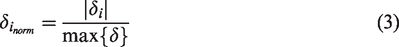
Shepard et al.²⁵ discussed the behaviour of gulls flying at different angles with the same radial distance to the buildings. Figure 14 presents two examples of this for WFD100. The resolution of the contour is 0.2 ms⁻¹ in all sub-figures, and the colorbar is kept constant for both wind fields, which is important to correctly interpret the results. The pairs A and B are situated at the same radial distance to the buildings at different angles. These points correspond to positions 7 and 22 from Figure 8, respectively.

Figure 14.

Comparison of two flight paths at the same radial distance from the buildings (A and B) with the distribution of the lateral (v) and vertical (w) wind vector components in relation to the building. Red error bars indicate the horizontal and vertical flight range of the SUAV during the simulation; the white bars show the standard deviation of the position error during flight. (a) and (b) present the effects of WFD100 of W20 = 2.26 ms^(-1) with a resolution of 0.2 ms^(-1) between levels. (c) and (d) show $WFD 100$ of W20 = 9.34 ms⁻¹ with a resolution of 0.2 ms⁻¹ between levels.

Figure 15.

Contour plots of mean throttle command and CE of control surfaces for WFD100 of $W 20 =$ 9.34 ms⁻¹ with the Dryden model altitude input set to a constant value of 30 m. The contour maps are based on the interpolation of successful flights, where red circles represent the flights that crashed against the ground or the buildings during simulation.

The comparison between the top and bottom figures (W20 = 2.26 ms⁻¹ and W20 = 9.34 ms⁻¹, respectively) highlights the difference between the spatial variation of the paths for the two wind fields. The wind gradient due to the horizontal displacement in the wind field is lower for the weakest wind field. This is due to the Dryden disturbance intensities being low. Therefore, the CE required to fly in this wind field is lower than the one required with W20 = 9.34 ms⁻¹. However, the wind gradient is proportional to the nominal wind speed, meaning that the wind field will have the same effect on the wind gradient in both cases but at different scales.

Figures 14(c) and (d) together with the discussion above suggest that position A requires more CE to hold vertical position in comparison to position B. The contour figures show that the lateral position of the SUAV moves across more w contours when flying at lower angles compared to at a higher altitude. This variation in the contour levels results in a greater wind gradient which is added to the Dryden disturbance model in the flight dynamics model.

Overall, the results suggest two things. First, they confirm that flying at a lower altitude and under stronger wind conditions requires more CE. Second, the magnitude of the wind components in the top figures compared to the bottom indicates that there is little benefit in terms of the required CE to flying in any specific region of the wind field at weaker nominal wind speeds, which was also shown in Figures 10 and 11 when looking at the magnitude of the CE required.

Shepard et al.²⁵ hypothesised that the gulls were flying at higher angles relative to the building in stronger winds in order to reduce their CE. This hypothesis is supported by the results of this study, with the CE required for the SUAV reducing with altitude and the mean throttle required increasing with radial distance from the front corner of the building. With this pattern of effects, the best compromise between reduced CE and reduced requirement for thrust production is to fly directly above the front corner of the building where the altitude is maximised for a given radial distance. However, at lower wind speeds, the gulls flew at lower angles out in front of the buildings, and this behaviour is not explained by this optimisation. When looking at the simulation results, it is apparent that in absolute terms, there is not much of a change in CE required with height at lower wind speeds so it may be that the gulls flew at lower angles to forage by the seafront, exploiting orographic lift whilst gaining a better view of the ground and find possible sources of food. This strategy may then become increasingly energetically costly as wind speed increases, along with having an increasing risk of collision with the buildings at higher wind speeds.

Conclusions

The work presented investigated the CE required for an SUAV to fly parallel to buildings whilst utilising orographic updraughts. The aim was to assess if there are any energetic benefits to flying in specific regions of the wind field. The WOT 4 Foam-E Mk2+ SUAV was simulated in Simulink to fly parallel to buildings by the seafront in Swansea. A range of different flight paths were imposed for a constant airspeed, and the CE and path displacement were calculated and discussed for two different wind fields affected by the Dryden disturbance model. Overall, the findings of this study indicate that:

The CE is correlated with the nominal wind speed and the level of disturbance added with the Dryden model.

The CE is mostly correlated with the inverse of the height at which the SUAV is flying.

Both strong and weak wind fields show a trend between the CE and the imposed height; however, at stronger nominal wind speeds, there is a greater advantage to flying at higher altitudes.

The mean throttle command varies with the radial distance to the buildings, showing a benefit of up to 15% in the throttle command when flying next to them as opposed to flying in the farthest path defined in this study. However, the simulations have shown that flying in this region of the wind field for strong nominal wind speeds increases the risk of collision with the buildings.

A strategy of flying directly over the front corner of the buildings appears to minimise the CE required for a given level of orographic lift and mirrors the behaviour of gulls seen at higher wind speeds.

Footnotes

Declaration of conflicting interests

The author(s) declared no potential conflicts of interest with respect to the research, authorship, and/or publication of this article.

Funding

The author(s) disclosed receipt of the following financial support for the research, authorship, and/or publication of this article: This project has received funding from the European Research Council (ERC) under the European Union’s Horizon 2020 research and innovation programme (grant agreement No 679355) and was supported by the EPSRC Centre for Doctoral Training in Future Autonomous and Robotic Systems (FARSCOPE) at the Bristol Robotics Laboratory.

ORCID iDs

Ana Guerra-Langan

Shane Windsor

References

Cai

Dias

Seneviratne

A survey of small-scale unmanned aerial vehicles: recent advances and future development trends. Unmanned Systems 2014; 2: 175–199.

Girard

Howell

Hedrick

JK.

Border patrol and surveillance missions using multiple unmanned air vehicles. In: 2004 43rd IEEE conference on decision and control (CDC) (IEEE Cat. No.04CH37601), Nassau, 2004, pp.620–625.

Tomic

Schmid

Lutz

, et al. Toward a fully autonomous UAV: research platform for indoor and outdoor urban search and rescue. IEEE Robot Autom Mag 2012; 19: 46–56.

CBP Public Affairs. U.S. Customs and Border Protection.

Qazi

Siddiqui

Wagan

AI.

UAV based real time video surveillance over 4G LTE. In: 2015 International Conference on Open Source Systems and Technologies (ICOSST), Lahore, 2015, pp.141–145.

Thiels

Aho

Zietlow

, et al. Use of unmanned aerial vehicles for medical product transport. Air MedJ 2015; 34: 104–108.

Murray

Chu

AG.

The flying sidekick traveling salesman problem: optimization of drone-assisted parcel delivery. Transport Res Part C: Emerg Technol 2015; 54: 86–109.

Yuan

Zhang

Liu

A survey on technologies for automatic forest fire monitoring, detection, and fighting using unmanned aerial vehicles and remote sensing techniques. Canadian J Forest Res 2015; 45: 783–792.

Erdelj

Natalizio

UAV-assisted disaster management: applications and open issues. In: 2016 International Conference on Computing, Networking and Communications (ICNC), Kauai, HI, 2016, pp.1–5.

10.

Bronz

Moschetta

Brisset

, et al. Towards a long endurance MAV. Int J Micro Air Veh 2009; 1: 241–254.

11.

Gavrilovic

Mohamed

Marino

, et al. Avian-inspired energy-harvesting from atmospheric phenomena for small UAVs. Bioinspir Biomimet 2019; 14: 1–20.

12.

Watkins

Milbank

Loxton

, et al. Atmospheric winds and their implications for microair vehicles. AIAA J 2006; 44: 2591–2600.

13.

Watkins

Thompson

Loxton

, et al. On low altitude flight through the atmospheric boundary layer. Int J Micro Air Veh 2010; 2: 55–68.

14.

Watkins

Fisher

Mohamed

, et al. The turbulent flight environment close to the ground and its effects on fixed and flapping wings at low Reynolds number. In: 5th European Conference for Aeronautics and Space Sciences (EUCASS), Munich, Germany, 2014, pp.1–10.

15.

Mohamed

Poksawat

Watkins

, et al. Developing a stable small UAS for operation in turbulent urban environments. In: International Micro Air Vehicle Conference and Flight Competition (IMAV), Toulouse, France, 2017, pp.184–189.

16.

Traub

LW.

Range and endurance estimates for battery-powered aircraft. J Airc2011; 48: 703–707.

17.

Shyy

Berg

Ljungqvist

Flapping and flexible wings for biological and micro air vehicles. Prog Aerosp Sci 1999; 35: 455–505.

18.

Langelaan

JW.

Long distance/duration trajectory optimization for small UAVs. In: AIAA Guidance, Navigation and Control Conference, Hilton Head, South Carolina, 2007, pp. 3654–3667

19.

White

Lim

Watkins

, et al. A feasibility study of micro air vehicles soaring tall buildings. J Wind Eng Indus Aerodyn 2012; 103: 41–49.

20.

White

Watkins

Lim

, et al. The soaring potential of a micro air vehicle in an urban environment. Int J Micro Air Veh 2012; 4: 1–13.

21.

Fisher

Marino

Clothier

, et al. Emulating avian orographic soaring with a small autonomous glider. Bioinspir Biomimet 2015; 11: 016002.

22.

Mohamed

Carrese

Fletcher

, et al. Scale-resolving simulation to predict the updraught regions over buildings for MAV orographic lift soaring. J Wind Engi Indus Aerodyn 2015; 140: 34–48.

23.

Watkins

Mohamed

Fisher

, et al. Towards autonomous MAV soaring in cities: CFD simulation, EFD measurement and flight trials. IntJ Micro Air Veh 2015; 7: 441–448.

24.

Tennekes

The simple science of flight: from insects to jumbo jets. Cambridge, MA: MIT Press, 2009.

25.

Shepard

Williamson

Windsor

SP.

Fine-scale flight strategies of gulls in urban airflows indicate risk and reward in city living. Philos Trans R Soc B: Biol Sci. Available at: https://doi.org/10.1098/rstb.2015.0394.

26.

Langelaan

JW.

Gust energy extraction for mini and micro uninhabited aerial vehicles. J Guid Control Dyn 2009; 32: 464–473.

27.

Depenbusch

NT.

Atmospheric energy harvesting for small uninhabited aircraft by gust soaring. PhD Thesis, Pennsylvania State University, Pennsylvania, USA, 2011.

28.

J.P. How. 16.333 Aircraft Stability and Control. MIT OpenCourseWare, Massachusetts Institute of Technology.

29.

Department of Defense. Flying Qualities of Piloted Aircraft. Department of Defense Handbook Mil-HDBK-1797B, 2012.

30.

Etkin

Dynamics of flight, stability and control. 2nd ed. Hoboken, NJ: John Wiley & Sons, 1982.

Unmanned aerial vehicle control costs mirror bird behaviour when soaring close to buildings

Abstract

Keywords

Introduction

Framework

Guidance

Navigation

Control

Limitations

Simulations

Wind field

Control effort

SUAV platform

Results and discussion

Conclusions

Footnotes

Declaration of conflicting interests

Funding

ORCID iDs

References