Sage Journals: Discover world-class research

Abstract

In this article, an optimal method of unmanned aerial vehicle selection for following a moving ground target is presented. The most suitable unmanned aerial vehicle from an aircraft operating fleet is selected for tracking task. The aircraft choice is done taking regarding the unmanned aerial vehicle distribution in the mission zone, individual performance of fleet platforms, and maneuverability of a ground platform. The unmanned aerial vehicle fleet members’ flying qualities are various, so an optimization process is used to assign an aircraft to follow the ground target. A target trajectory prediction is embedded in tracking algorithm. The simulation results demonstrated the effectiveness of algorithms developed, and in-flight demonstration proved the possibility of realization of computed trajectories by the unmanned aerial vehicle.

Keywords

Adaptive control optimization flight control system simulation control engineering

Introduction

A tracking of moving objects by unmanned aerial vehicles (UAVs) is investigated by many authors.^1–4 In this research, the tracking task was a part of wider mission that contains three phases: Locate, Target, and Track (LTT). The optimization of Locate and Target tasks was subject to other research optimized within the project OpUSS—“Optimization of Unmanned System of Systems”—performed at Warsaw University of Technology under a research grant agreement with Lockheed Martin Corporation. The main objective of OpUSS project was to create and implement a methodology that optimizes the performance of a UAV fleet for the LTT mission at each phase. It was realized using multilevel optimization methods for each task of the LTT mission. For the Track task, the optimization was used for the selection of the most proper and useful UAV for following the moving object and generation of tracking trajectory. The optimization of third—Track—task is presented in this article. The novelty of the research shows multilevel optimization, taking into account as well the model of the UAVs and the estimation of the escaping object’s trajectory. The presented method considers the UAV’s performance and fuel/energy resources. The main difficulty of the research was to apply such an algorithm that may be used onboard, so the calculation can be done in real time. The algorithm and method were developed and tested in virtual environment (computer simulations), but to prove its applicability, the method was applied in real flight, with the use of set of various UAVs.

One of the key elements of optimization was the selection of the best aircraft for tracking. The process takes into account the performance and maneuverability of each fleet member, actual positions of aircraft, and estimated available flight time durations based on remaining fuel/energy consumption.

There are several references published, which concern target tracking. In some of them, stochastic methods^1,3,5 were used for generating tracking trajectory; in others, a deterministic approach^2,4 was investigated. To optimize the path of a tracking vehicle, various methods were used, such as Markov decision processes¹ or dynamic programming.^6–8 In this article, an approach used to solve the tracking problem is delivered. Next, the method of selection of an optimal aircraft for tracking is described, followed by a description of UAV/target models, track algorithm, and target motion prediction method. The simulation findings illustrate the applicability and effectiveness of the algorithms developed, and flight tests proved the applicability of the results in practice.

UAV optimal selection for tracking phase

The non-moving object on the ground was searched in the mission zone and has been identified by a member of UAV fleet. Being found, the object starts moving on the ground. This is the initial situation for research described in this article. A decision must be undertaken which UAV from in-the-air operating fleet over the mission area will be used to track the running object. The followed object performance is known in general, but its trajectory is not known in advance by the tracking fleet and may vary during the Track phase. The main factors taken into account, which influence the selection of UAV for tracking, are as follows:

Fleet distribution in the mission area when the target is detected;

Estimated remained flight duration of each UAV performing tracking, based on fuel/energy consumption and assumed the “worst” target escaping trajectory;

UAV maneuverability depending on UAV type, which is attached to the UAV model;

Target maneuverability, which is considered in an object model.

The main criterion for selection of an optimal aircraft is the estimated tracking time duration, depending on fuel/energy consumption. The fuel consumption is considered in both mission phases: reaching the target and tracking the target.

An UAV and an object trajectory are considered as a movement on a two-dimensional (2D) space, which means that the UAV altitude is constant. An example of random fleet distribution over the mission area when an object was found is presented in Figure 1. The distances of UAVs to the object and its initial position are presented. The UAV are placed randomly, and their distances $d_{AT, i}$ to the target are

d_{A T, i} = \sqrt{{(x_{a i} - x_{T})}^{2} + {(y_{a i} - y_{T})}^{2}}

(1)

Figure 1.

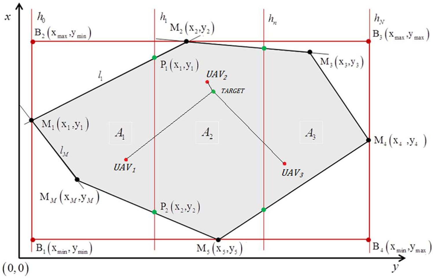
Search area definition.

The fuel/electrical energy consumption by a UAV is estimated by the following formulas:

For piston engines

Δ m_{F i} = q_{e i} \cdot \frac{d_{A T, i}}{v_{a i}} \cdot N (v_{a i})

(2a)

For electrical engines

Δ Q = \frac{d_{A T, i}}{v_{a i}} \frac{N (v_{a i})}{η U (Q)}

(2b)

where $q_{e}$ is the specific fuel consumption. The N parameter represents the power required to maintain required speed, $η$ is the efficiency of the electric drive, U is the voltage on energy source, and $v_{opt}$ is the UAV velocity selected to reach starting tracking position. The power that is required to maintain specified altitude and velocity is represented by an equation

N_{t, i} = \frac{ρ {(v_{a, i})}^{3}}{2} S C_{D, i}

(3)

By inserting equation (3) into equation (4), the following expressions for fuel/energy consumption is delivered

\begin{array}{l} Δ m_{F i} = ρ d_{A T, i} {(v_{a, i})}^{2} [q_{e, i} \frac{1}{2} S C_{D, i}] or \\ Δ Q = ρ d_{A T, i} {(v_{a, i})}^{2} [\frac{1}{2 η U} S C_{D, i}] \end{array}

(4)

The crucial factors that have an impact on the fuel/energy consumption are air density, distance flown, flight velocity $v_{a, i}$ , and UAV characteristics like propulsion efficiency and aircraft aerodynamics. To begin tracking phase, the selected UAV has to get to the initial tracking position. In the research, it was assumed that the trajectory to the target will be a straight line and its velocity $v_{a, i}$ will be constant. In this part of task, UAV would consume a specified amount of fuel/energy $Δ m_{F, i} or Q_{i}$ . An estimated tracking time $t_{track, i}$ during which an UAV may follow the target depends on the target motion and the tracking strategy realized by aircraft, which result in a distance $d_{i}$ flown by UAV with velocity $v_{a, i}$ . To select the UAV which is best for tracking, the tracking time is estimated using the algorithm for target following (described in subsequent part of this article), which will be used to track the object, and its trajectory is chosen from a certain class of trajectories consistent with its maneuverability.

Vehicle models

In the literature, various models of vehicle motion may be found for trajectory optimization processes, like Dubins car,^9,10 full dynamics aircraft model,¹¹ or models based on transfer functions^12–15 identified during tests in flight. In optimization processes, the model complexity influences the selection of an applied method and computation time. Usually, for simulation efficiency, the applied model is not very complex. This is the case in this research, but the software structure allows to make it more comprehensive in the future research. An UAV and the object to find are modeled as a maneuvering point. An UAV flies at a fixed altitude. Both—UAVs’ and object’s—trajectories are expressed by two parametric equations in horizontal plane of north-east-down (NED) coordinate system

\begin{matrix} x_{a} = x_{a} (t) & x_{T} = x_{T} (t) \\ y_{a} = y_{a} (t) & y_{T} = y_{T} (t) \end{matrix}

(5)

UAV and object motion are presented by kinematic equations

{\dot{x}}_{a} = v_{a} \cos (ψ_{a}), {\dot{x}}_{T} = v_{T} \cos (ψ_{T})

(6)

{\dot{y}}_{a} = v_{a} \sin (ψ_{a}), {\dot{y}}_{T} = v_{T} \sin (ψ_{T})

(7)

{\overset{\cdot}{y}}_{a} = v_{a} \sin (ψ_{a}), {\overset{\cdot}{y}}_{T} = v_{T} \sin (ψ_{T})

(8)

{\overset{\cdot}{ψ}}_{a} = Ω_{a} = \frac{v_{a}}{R_{a}}, {\overset{\cdot}{ψ}}_{T} = Ω_{T} = \frac{v_{T}}{R_{T}}

(9)

The UAV is subjected to constraints imposed on:

Horizontal velocity: minimal $v_{a, min}$ because of the stall conditions and maximum $v_{a, max}$ —power constrains

v_{a, min} \leq v_{a} \leq v_{a, max}

(10)

Roll angle—stall constrains

0 \leq | φ_{a} | \leq φ_{a, max}

(11)

The minimum turn radius calculated as

R_{a, min} = \frac{v_{a}^{2}}{g \sqrt{n_{max}^{2} - 1}}

(12)

Aircraft turn radius may also be taken from measures in experimental flights. Target velocity is constrained by maximum engine power

v_{T} \leq v_{T, max}

(13)

An algorithm for target following

The object following algorithm is a deterministic one, based on the method developed in Rafi et al.² and Ruangwiset.⁴ In Figure 2, parameters crucial for the tracking algorithm are illustrated. Point $A (x_{a}, y_{a})$ is the aircraft actual position and point $T (x_{T}, y_{T})$ is the target estimated position in the next time step. An object circle is drawn with the center in target position and radius $r_{TARGET}$ equals to a minimum aircraft turn radius $R_{a, min}$ . The relative distance $β$ of aircraft to the target is defined as

β = \frac{d_{A \hat{T}}}{r_{TARGET}}

(14)

Figure 2.

Bearing selection.

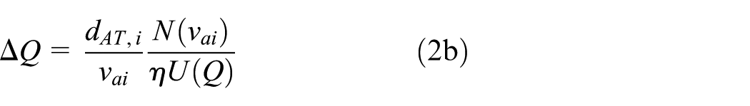
At each time step, calculations are done as follows:

Actual target position $T (x_{T, t}, y_{T, t})$ is determined (using aircraft sensors) during the actual instant of time t;

Predicted target position $\hat{T} (x_{T, est, t + 1}, y_{T, est, t + 1})$ in the next time step t + 1 is calculated using algorithm for prediction of target motion;

Heading change $Δ ψ_{a, t}$ of the aircraft located in point $A (x_{a, t}, y_{a, t})$ is calculated, which depends on predicted target position $\hat{T} (x_{T, est, t + 1}, y_{T, est, t + 1})$ and the distance to the predicted target position $d_{A \hat{T}, i}$ , expressed in a non-dimensional form as parameter $β$ ;

The UAV position in consequent step is calculated using aircraft model

\begin{matrix} x_{at + Δ t} = x_{a, t} + v_{a} \cos (ψ_{a, t} + Δ ψ_{a, t}) Δ t \\ y_{a, t + Δ t} = y_{a, t} + v_{a} \sin (ψ_{a, t} + Δ ψ_{a, t}) Δ t \\ ψ_{a, t + Δ t} = ψ_{a, t} + Δ ψ_{a, t} \end{matrix}

(15)

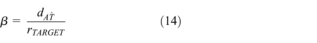
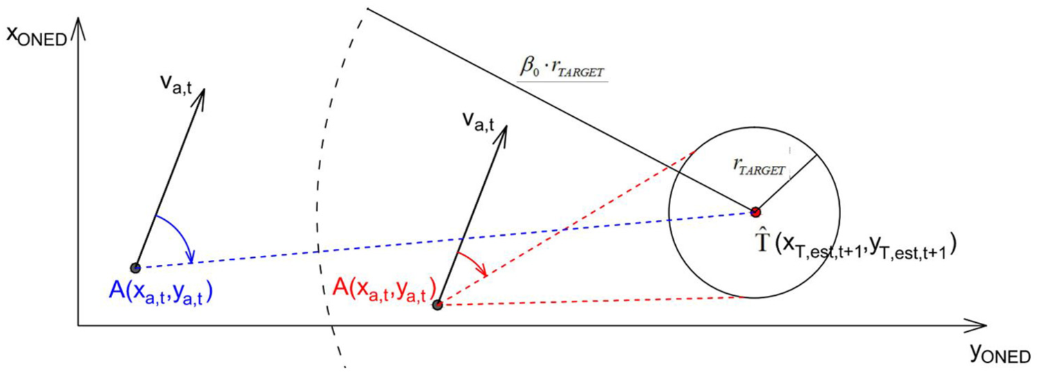
The heading changes along the UAV, and depends on the actual value of parameter β, that is, the relative distance between UAV and the object. The fixed β₀ value was assumed to improve the algorithm efficiency. For each instant of time one of the three cases may be encountered:

The UAV is inside an object circle, that is, 0 < β < 1. If so, the heading rate is constant and does not change, $Δ ψ_{a, t} = 0$ .

The UAV is outside the object circle, however closer than assumed relative distance β₀, that is, if 1 < β < β₀. In this case, the target tracking algorithm described below is applied.

The UAV is further than β₀, that is, β > β₀. If so, the aircraft heading is selected straight to the target (a dotted line AT in Figure 3).

Figure 3.

Target tracking algorithm steps.

The object following algorithm developed here and applied in case 2 is described now. In Figure 4, point $A (x_{a}, y_{a})$ is an actual UAV position, and point $T (x_{Test}, y_{Test})$ is a predicted target position in a next instant of time. The target circle is drawn around the target predicted position $T (x_{Test}, y_{Test})$ . The lines AT₁ and AT₂ tangent to the target circle are drawn from actual aircraft position (point $A (x_{a}, y_{a})$ ). The aircraft velocity vector is $v_{a}$ . The UAV heading change is calculated as the lower value of one of the two bearings of the tangent lines τ₁ and τ₂

τ = min (τ_{1}, τ_{2})

(16)

Figure 4.

Mean and maximum distances to the target as a time step function.

To calculate the angles τ₁ and τ₂, the bearing $δ$ to predicted target position is calculated as

\begin{array}{l} \sin δ = \frac{| v_{a} \times d_{A \hat{T}} |}{v_{a} \cdot d_{A \hat{T}}} = \frac{v_{a} \cdot d_{A \hat{T}} \cdot \sin (v_{a}, d_{A \hat{T}})}{v_{a} \cdot d_{A \hat{T}}} \\ = \sin (v_{a}, d_{A \hat{T}}) \end{array}

Angles τ₁and τ₂ are calculated as

τ_{1} = δ - Δ τ, τ_{2} = δ + Δ τ

(17)

and the incremental change $Δ τ$ is calculated as

Δ τ = \arcsin \frac{r_{TARGET}}{d_{AT'}}

(18)

where $d_{A \hat{T}, t} = \sqrt{{(x_{T, est, t + 1} - x_{a, t})}^{2} + {(y_{T, est, t + 1} - y_{a, t})}^{2}}$ the distance $d_{A \hat{T}}$ between the UAV actual position and object’s predicted position in the next time step. When the bearing is selected, an algorithm decides about the heading change in the current time step. And so, if the $τ (t) < | Δ ψ_{a, max} |$ dependency is true, then

Δ ψ_{a, t} = \pm τ_{t}

(19)

else

Δ ψ_{a, t} = \pm Δ ψ_{a, max}

(20)

If the actual angle between aircraft velocity vector and the tangent direction is smaller than a maximum change of an aircraft turn angle in one time step, then the heading change is $τ_{t}$ . Otherwise, the UAV changes its heading $Δ ψ_{a, max}$ . The object position prediction in the following time step is an element of tracking algorithm, proposed in this study. There are many methods used to predict target motion, for instance.^4,16 Usually, the past object’s motion knowledge is used. Thanks to the modular algorithm structure, the various prediction methods can be applied and tested. In presented research, a deterministic extrapolation is applied, where the last time step data are used to estimate the object’s trajectory using the object’s model

ψ_{T, est, t + 1} = ψ_{T, t}

(21)

x_{T, est, t + 1} = x_{T, t} + v_{T, t} \cos ψ_{T, t} Δ t

(22)

y_{T, est, t + 1} = y_{T, t} + v_{T, t} \sin ψ_{T, t} Δ t

(23)

The advantages of presented method are that it is not necessary for extensive onboard calculations and a fact that a deterministic approach assures the solution repeatability for constant parameters.

Simulation results

In this section, the results of simulation of the tracking algorithm are summarized within two groups of calculations. First one concerns the assessment of dependence of the target tracking algorithm results on the algorithm internal parameters:

Time step $Δ t$ ;

Relative distance to the target $β_{0}$ ;

Target circle radius $r_{TARGET}$ .

The second group concerns sample computations of tracking paths for various UAVs and target motion parameters. Finally, comparison of simulated trajectories with experimental flight results is presented. All calculations were done using MATLAB R2014b software. To assess the quality of tracking process, two indicators were calculated for the whole duration of the tracking task—first one, a mean distance to the target

d_{mean} = \frac{\sum_{t = 0}^{T} d_{AT} (t)}{T} Δ t

(24)

where $d_{AT} (t)$ is a distance to the target at the moment t, T is the total tracking time and $Δ t$ is the time step size reflecting sampling time of the onboard sensors; the mean distance to the target reflects possibility and quality of monitoring the target behavior. And, the second indicator, a maximum distance to the target

d_{max} = max_{t \in 〈 0; T 〉} (d_{AT} (t))

(25)

which indicates whether the target is all the time within the sensor field of view. To test the algorithm properties, three different aircraft models were used, due to their availability for flight tests; the aircraft performance data are given in Table 1.

Table 1.

Aircraft performance data.

	REKIN	CITABRIA	T-REX
Aircraft type	Fixed-wing	Fixed-wing	Rotorcraft
Propulsion type	Electrical motor	Internal combustion engine	Electrical motor
Best endurance velocity (m/s)	22.8	25	5
Turn radius (m)	40	70	10

Investigation of algorithm properties

In this section, the target tracking algorithm sensitivity to its internal parameters is discussed. There are three algorithm internal parameters crucial for simulation efficiency: $Δ t$ is the time step size; $β_{0}$ is the relative distance to the target, according to which an aircraft changes its tracking strategy; and radius of the target circle $r_{TARGET}$ . A size of a time step $Δ t$ reflects a sampling time of onboard sensor, which is also related to computing power needed for the realization of algorithm online. Minimum duration of the time step is selected depending on sensor sampling frequency, aircraft velocity, and time of computations to be performed in one time step. The last factor turned out to be non-crucial in our application (max computing time for one step was 0.07 (s)).

Assuming a constant velocity of an aircraft, the time step was changed within range from 0.1 to 2 s. Other values set in simulation are given in Table 2.

Table 2.

Simulation parameters (time step).

Parameter	Value
Selected aircraft	REKIN (fixed-wing)
Trajectory	Straight line
Target velocity	5 m/s (constant)
Transition value of the relative distance	2

The time step duration significantly influences the maximal distance, but not so much the mean to the target (Figure 4). The longer is a time step, the greater is the maximum distance to the target; for time step of 2 s, it is about 56% larger than for time step of 0.1 s. Increasing the time step results in slightly larger mean distances to the target (23% more for 2 s than for 0.1 s).

The tracking trajectories obtained for 0.1 and 2 s time steps are compared in Figure 5. The larger time step results in the deterioration of algorithm performance (longer trajectories), which is coherent with engineering understanding of the process. Such a situation may appear when a sampling time in an onboard sensor, which reflects the distance and relative position to the target, is high due to sensor performance or severe weather conditions.

Figure 5.

Aircraft trajectories for time step t = 0.1 s and t = 2 s.

The parameter $β_{0}$ is a relative distance to the target with respect to the aircraft turn radius, influencing aircraft tracking strategy. As the value of this parameter is chosen arbitrary, only detailed simulations for the specific cases may provide conclusive results of the impact of this parameter on tracking quality. It is expected that for each UAV—target case, it is possible by simulations to find an optimal value of $β_{0}$ , which ensures the best tracking performance. An influence of $β_{0}$ was checked for fixed-wing UAV (REKIN) and rotorcraft (T-REX). The simulation parameters for investigating the influence of $β_{0}$ are given in Table 3, and simulation results are presented in Figure 6.

Table 3.

Simulation parameters (relative distance).

Parameter	Value
Selected aircraft	REKIN (fixed-wing) and T-REX (rotorcraft)
Trajectory	Straight line
Target velocity	5 m/s
Time step	0.1 s

Figure 6.

Mean and maximum distances to the target in β₀ function.

For both cases, the influence of this parameter on tracking efficiency is not substantial. For REKIN aircraft, larger $β_{0}$ gives smaller maximum (1.5% less for maximum values) and smaller mean distance to the target (6.7% less). However, there is a transition range of $β_{0}$ where the values of these quality indicators are significantly higher (up to 12.5% more) in the region of 1.5 relative distance to the target. It seems that for a particular case, such a region should be identified and avoided. For rotorcraft, increasing the relative transition distance results in a slightly greater tracking maximum distance (2.3% more) and in a smaller mean distance to the target (3.4%). The parameter $r_{TARGET}$ is the radius of the “target circle,” which was assumed to be equal to the minimal turn radius of the tracking aircraft. It was interesting to assess the algorithm efficiency dependence on the ratio of turn radius to target circle radius ratio $R_{min} / r_{TARGET}$ . It may be expected that the best value of these ratios may be found in terms of fuel/energy consumption and total tracking time. To check the impact of the target circle radius, it was combined with aircraft turn radius as a non-dimensional parameter

Π = \frac{r_{TARGET}}{R_{a, min}}

(26)

The value of $Π$ used in the previous simulations was equal to 1; therefore, current set of simulations tested the algorithm performance for other values of $Π$ . The simulation parameters for $Π$ simulation are given in Table 4, and the simulation results are presented in Figure 7.

Table 4.

Simulation parameters (target circle radius).

Parameter	Value
Selected aircraft	REKIN (fixed-wing)
Trajectory	Straight line
Target velocity	5 m/s
Time step	0.1 s

Figure 7.

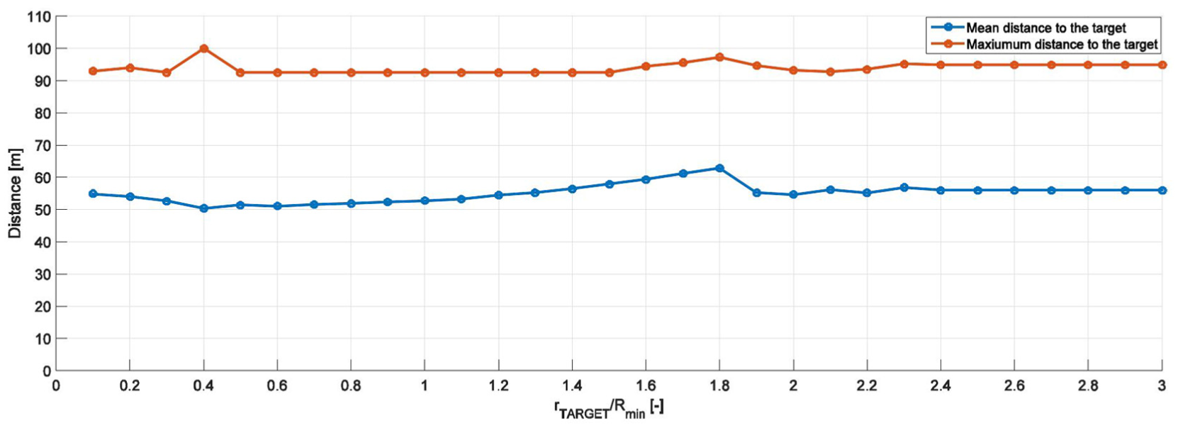
Mean and maximum distances to the target in Π function.

When increasing the value of $Π$ parameter, the maximum distance to the target is slightly changed with a tendency to increase for greater $Π$ values. The value of the mean distance to the target is increasing, until $Π = 1.8$ , then it drops about 12% and stays constant. Comparing to the case of the value $Π = 1$ assumed previously, the values of mean distances are smaller for $Π \in 〈 0.3; 0.9 〉$ . This indicates that by the selection of “tracking radius,” the tracking performance may be influenced and improved. However, it still requires simulations to get better insight into the impact of $Π$ for other target trajectories and other UAVs.

UAV/target motion parameters

In this section, the influence of target trajectories and target/aircraft velocity ratio $v_{T} / v_{a}$ is investigated. A target trajectory influenced significantly the aircraft trajectory, as there is close relation between these two motions. The simulations were performed for various aircraft models and for two trajectories: straight line and zig-zag composed of straight segments. The simulation was performed for three different UAVs (see Table 5).

Table 5.

UAV performance used in simulation.

Aircraft type	Performance
T-REX (rotorcraft)	$v_{a} = 6 m / s, R_{a} = 10 m$
REKIN (fixed-wing)	$v_{a} = 6 m / s, R_{a} = 40 m$
CITABRIA (fixed-wing)	$v_{a} = 6 m / s, R_{a} = 70 m$

UAV: unmanned aerial vehicle.

The tracking trajectories are presented in Figure 8.

Figure 8.

Trajectories for straight-line target trajectory: T-REX—green, REKIN—blue, and CITABRIA—yellow.

T-REX (helicopter) has available velocity only slightly larger than the target; therefore, it is compensated by making sinusoidal movements, sufficient to directly follow the target. The airplanes (fixed-wing): REKIN and CITABRIA due to much higher flight velocities compared to the target velocity perform loiter around moving point.

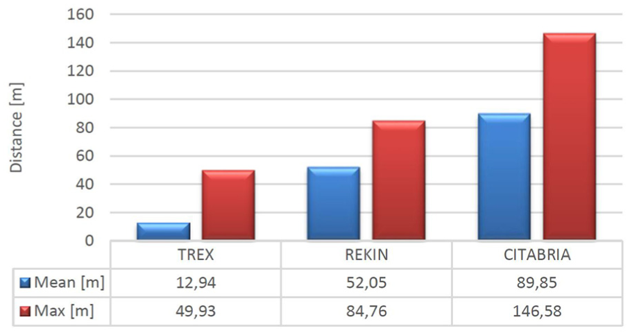
In Figure 9, the tracking quality indicators are presented for each case shown in Figure 9. The higher mean and maximum distances to the target for quicker flying aircraft are intuitively explainable, which prove that the algorithm operations are proper. A similar analysis was done for zig-zag trajectory. In Figure 10, trajectories for all three UAVs are shown.

Figure 9.

Mean and maximum distances to the target for all UAVs for straight-line target trajectory.

Figure 10.

Trajectories for zig-zag target trajectory: T-REX—green, REKIN—blue, and CITABRIA—yellow.

The zig-zag “non-smooth” target trajectory has larger influence on rotorcraft than on fixed-wing UAVs, which results from velocity ratios. In the zig-zag corners, helicopter needs more time to reach the target than the fixed-wing loitering around the target.

The comparison of maximal and mean distances to the target for zig-zag trajectories, presented in Figure 11, reveals the same trends as in the straight-line case. But, there is largest relative change for T-REX, which suggests that the quality of tracking by rotorcraft is influenced by the shape of trajectories more than fixed-wing.

Figure 11.

Mean and maximum distances to the target for all UAVs for zig-zag target trajectory.

Velocity ratio

In this section, the algorithm behavior is investigated for various target/UAV velocity ratios $v_{T} / v_{a}$ . From this part of the simulations, additional guidance for selecting the aircraft best suited to track the specified target may be expected. It was assumed that the constant UAV velocity is 22.8 m/s, and the target velocity is changed from 1 to 21 m/s every 1 m/s. In Figure 12, mean and maximum distances to the target are presented as a function of relative target/aircraft velocity ratio.

Figure 12.

Mean and maximum distances to the target as a velocity ratio function.

For the velocity ratio $v_{T} / v_{a} = 0.65$ , the tracking quality parameters encounter substantial change, which results from changing the tracking strategies. From this plot, some practical conclusions may be drawn. It is important to select the aircraft velocity to be comparable with the target velocity. In the case where it is not possible, aircraft velocity should be as high as possible. It may be recommended to avoid velocity ratio in range of 0.2–0.75. The conclusions above depend on aircraft and target performances, so such calculations should be done to define the best aircraft velocity from the mean and the maximum distances to the target.

Comparison between simulation and experimental flights

In this section, the simulated trajectories are compared with demonstrations in flight. The tracking trajectories were calculated for rotorcraft UAV (T-REX) flying with horizontal velocity of 4.5 m/s, tracking the target moving along the straight line with constant velocity of 3 m/s. On the simulated trajectories, the waypoints were selected, with mean distance between two simulated waypoints were about 10–15 m and downloaded to rotorcraft autopilot. The helicopter flight trajectories with respect to required waypoints are presented in Figure 13. The rotorcraft followed the waypoints with assumed accuracy of 15 m. This result proves the applicability of computed for real tracking flight. In Figure 14, the distance is shown between points of helicopter trajectory obtained from simulation and nearest points from experiment. The mean distance to the reference (simulation) trajectory was 2.33 m and the maximum inaccuracy was 6.64 m.

Figure 13.

Simulated and experimental trajectories comparison.

Figure 14.

Distance between simulated and experimental trajectory points.

Conclusion

The tracking of a ground-moving platform by an UAV is considered in the article. The tracking algorithm starts with the first step—a method for selection of the best UAV from the fleet distributed throughout the mission zone, based on one-step optimization. The kinematic models of aircraft and target are used, including their maneuverability. The objective of optimization is to achieve the longest tracking time taking into account the actual fuel/energy consumption. The tracking algorithm was developed considering the aircraft maneuverability, which significantly have an impact on the tracking trajectory. The algorithm properties were investigated showing efficiency in performing tracking for various types of UAVs. Having such strong results, the simulation could be taken into the real flight tests. The presented method’s complexity is not high, so its applicability in real flight was possible. Due to the algorithm simplicity, the calculation could be performed onboard. The test on an airfield has been performed and the applicability of simulation results was proved by demonstration in flight with the use of various UAVs fleet. Further research would consider applying the method and integrating the estimating the trajectory along with the sensors feedback (cameras and lasers). Furthermore, the method’s applicability should be tested for a wider spectrum of various UAVs.

Footnotes

Appendix 1

Handling Editor: Dumitru Baleanu

Declaration of conflicting interests

The author(s) declared no potential conflicts of interest with respect to the research, authorship, and/or publication of this article.

Funding

The author(s) disclosed receipt of the following financial support for the research, authorship, and/or publication of this article: This paper was prepared within project OpUSS—Optimization of Unmanned System of Systems—performed at Warsaw University of Technology under research grant agreement with Lockheed Martin Corporation supported by Drs Derreck Holian and Karen Duneman.

ORCID iD

Antoni Kopyt

References

Baek

Kwon

Yoder

et al . Optimal path planning of a target-following fixed-wing UAV using sequential decision processes. In: Proceedings of the 2013 IEEE/RSJ international conference on intelligent robots and systems (IROS), Tokyo, Japan, 3–7 November 2013. New York: IEEE.

Rafi

Khan

Shaﬁq

et al . Autonomous target following by unmanned aerial vehicles. In: Proceeding of SPIE defense and security symposium, Orlando, Florida, May 2006.

Peng

Zhao

Lin

et al . Vision based target tracking/following and estimation of target motion. In: Proceedings of the AIAA guidance, navigation, and control conference (AIAA Paper No.2013–5036), Boston, MA, 19–22 August 2013. Reston, VA: AIAA.

Ruangwiset

. Path generation for ground target tracking of airplane-typed UAV. In: Proceedings of the 2008 IEEE international conference on robotics and biomimetics, Bangkok, Thailand, 22–25 February 2009. New York: IEEE.

. Probabilistic path planning for cooperative target tracking using aerial and ground vehicles. In: Proceedings of the American control conference, San Francisco, CA, 29 June–1 July 2011. New York: IEEE.

Kim

Moving ground target tracking in dense obstacle areas using UAVs. In: Proceedings of the 17th World Congress the international federation of automatic control, Seoul, Korea, 6–11 July 2008. New York: IEEE.

Quintero

SAP

Papi

Klein

et al . Optimal UAV coordination for target tracking using dynamic programming. In: Proceedings of the 49th IEEE conference on decision and control, Atlanta, GA, 15–17 December 2010. New York: IEEE.

Bayat

Mobayen

Javadi

Finite-time tracking control of nth-order chained-form non-holonomic systems in the presence of disturbances. ISA T 2016; 63: 1–14.

Witkowski

Proposed algorithms for mission planning for groups of UAVs: European seventh framework programme FP7–218086-collaborative project, 2010, http://www.indect-project.eu/files/deliverables/public/Deliverable%202.7.pdf/view

10.

Shanmugavel

Tsorudos

White

et al . Co-operative path planning of multiple UAVs using Dubins paths with clothoid arcs. Control Eng Pract 2010; 18: 1084–1092.

11.

Chen

et al . Coverage path planning for UAVs based on enhanced exact cellular decomposition method. Mechatronics 2011; 21: 876–885.

12.

Lin

Goodrich

. UAV intelligent path planning for wilderness search and rescue. In: Proceedings of the IEEE/RSJ international conference on intelligent robots and systems, St. Louis, MO, 10–15 October 2009. New York: IEEE.

13.

Yang

Polycarpou

Minai

Multi-UAV cooperative search using an opportunistic learning method. J Dyn Syst: T ASME 2013; 129: 716–728.

14.

Santamaria

Segor

Tchouchenkov

et al . Path planning for rapid aerial mapping with unmanned aircraft systems. In: Proceedings of the international conference on systems (ICONS), Seville, 31 January–1 February 2013. Red Hook, NY: Curran Associates.

15.