A monolithic algorithm for the flow simulation of flexible flapping wings

Abstract

It has been a challenge to simulate flexible flapping wings or other three-dimensional problems involving strong fluid–structure interactions. Solving a unified fluid–solid system in a monolithic manner improves both numerical stability and efficiency. The current algorithm considered a three-dimensional extension of an earlier work which formulated two-dimensional fluid–structure interaction monolithically under a unified framework for both fluids and solids. As the approach is extended from a two-dimensional to a three-dimensional configuration, a cell division technique and the associated projection process become necessary and are illustrated here. Two benchmark cases, a floppy viscoelastic particle in shear flow and a flow passing a rigid sphere, are simulated for validation. Finally, the three-dimensional monolithic algorithm is applied to study a micro-air vehicle with flexible flapping wings in a forward flight at different angles of attack. The simulation shows the impact from the angle of attack on wing deformation, wake vortex structures, and the overall aerodynamic performance.

Introduction

Fluid–structure interaction (FSI) is inevitable in the study of dynamic behaviors in nature and engineering applications. Due to its complexity involving both fluid flows and flexible structures, FSI is usually studied in a progressive manner: first one-way coupling, then two-way coupling but with rigid-body motion, and eventually two-way coupling with visco-elastic solid structures. One example is the century-long study of (flexible) flapping-wing flight mechanism involving strong FSI between air and wings. The basic mechanism of the thrust generation from flapping wings is described independently by Knoller ¹ and Betz ² more than a century ago. The difference in thrust generation from pure plunging and pitching was first studied by Garrick. ³ More recently, there were studies^4–7 considering “onsideri impact from moving structures to fluid flow. With the need to understand the impact of flexibility on flapping-wing aerodynamics in modern technologies,^8–16 it becomes crucial to explore the physics of two-way fully coupled FSI problems computationally and experimentally.

Numerical simulation of a fully coupled FSI problem typically includes two separate sets of equations, algorithms and modularized computer codes, for fluid and solid, respectively. The coupling of the two parts is achieved by an iterative process of exchanging information at the fluid–solid interface.^17–20 During the process, other algorithms may be involved for the projection and mapping between different coordinate systems for the computation of fluid flows and solid structures. Despite the convenience from separating the code development on fluid and solid solvers, this common practice faces challenges in computational efficiency and stability. The projection and exchange at the fluid–solid interface may potentially reduce the overall efficiency and may not reach the convergence with an iterative process at each time step. Physically, the response in fluids and solids are largely different in time scale, and the smaller time scale may limit the overall time to reach the convergence at the fluid–solid interface and therefore reduce the computational efficiency. An ideal remedy would be to have a unified description and a monolithic algorithm to solve the entire FSI problem simultaneously without iterations.

The presented monolithic approach is based on a unified fluid–solid equation in an Eulerian configuration for a combined domain of fluids, solids, and the interfaces.^10,21,22 The immersed boundary method^23–32 was implemented relying on surface-force and body-force terms to represent the fluid–structure boundaries and the structural dynamics for viscoelastic bodies with one simple discretization. On the other hand, to assure the accuracy in the computation of structural dynamics, a Lagrangian mesh is kept to track the location of the structure. In the current work, the elastic stress in solids, at the expense of a projection process between fluid and solid,^10,21 gets more sophisticated for three-dimensional systems. When the situation requires a prescribed motion for certain solid structures (e.g. control gear in mechanical system, or skeleton system in a flying bird),^10,31 the aforementioned formulation allows additional terms to define motion trajectory in a way similar to traditional immersed boundary method.^26,30

The rest of the paper introduces the basic idea and derivation of the unified governing equations for fluids and solids. Followed by the governing equations, a detailed description of various algorithms is presented to deal with numerical challenges in the implementation of the unified fluid–solid equation. The focus is to explain the theoretical derivation and computational treatment of elastic stress terms during the cell division and the projection between the Eulerian and Lagrangian coordinates. Two benchmark cases were demonstrated to validate the algorithm in three dimensions and the viscoelastic treatment in two dimensions. Finally, the current monolithic approach for FSI systems was applied to simulate the flow surrounding the flexible flapping wings of a micro-air vehicle (MAV), which involves all the fundamental features provided by the current algorithm: three-dimensional system, passive viscoelastic structure (i.e. the wing), actively prescribed motion (i.e. the control gear for flapping mechanism). In this study of a flapping-wing forward flight, different angles of attack are considered for the impact on wing deformation, flow structures, and the overall aerodynamic performance. A concise discussion concludes this work.

Governing equations

The whole region is divided into two parts: the fluid region Ω _f and the solid region Ω _s . The solid region Ω _s is further divided into two parts, the prescribed region Ω _sp and the free passive region Ω _sf , as shown in Figure 1. In other words, $\Omega ={\Omega }_f\cup {\Omega }_s$ and ${\Omega }_s={\Omega }_{\mathit{sp}}\cup {\Omega }_{\mathit{sf}}$ . The whole region Ω is formulated in an Eulerian coordinate, while the solid region Ω _s is tracked in a Lagrangian manner. The combined governing equations for both incompressible solids and fluids can be expressed in a unified format under the Eulerian configuration.

Figure 1.

Sketch of different regions in a unified fluid–solid domain: the fluid region Ω _f , the solid region Ω _sf with free passive motion, and the solid region Ω _sp with actively prescribed motion.

Eulerian description for fluids

For an incompressible fluid, the non-dimensional continuity and momentum equations must be satisfied

$$\nabla ·{\mathbf{u}}_f=0$$

(1)

$$\rho \frac{D{\mathbf{u}}_f}{\mathit{Dt}}=\nabla ·{\mathit{\sigma }}_f$$

(2)

where the Cauchy stress for incompressible fluids ${\mathit{\sigma }}_f$ includes pressure p and dissipative viscous stress ${\mathit{\tau }}_f$

$${\mathit{\sigma }}_f=-p\mathbf{I}+{\mathit{\tau }}_f$$

(3)

For a Newtonian fluid, the dissipative viscous stress tensor can be derived by employing Onsagerng reciprocal relations and Coleman–Noll procedure in Clausius–Duhem inequality as ³³

$${\mathit{\tau }}_f={\mu }_f(\nabla {\mathbf{u}}_f+\nabla \mathbf{u}\mathit{fT})$$

(4)

By substituting equations (3) and (4) into equation (2), the celebrated Navier–Stokes equations for incompressible viscous flows can be found

$$\nabla ·{\mathbf{u}}_f=0$$

(5)

$$\frac{\partial {\mathbf{u}}_f}{\partial t}+{\mathbf{u}}_f·\nabla {\mathbf{u}}_f=-\nabla p_f+\frac{1}{R{e}_f}{\nabla }^2{\mathbf{u}}_f$$

(6)

where ${\mathbf{u}}_f$ is the velocity vector for fluid, t is time, p is pressure, and $R{e}_f={\rho }_f{U}_{\infty }L/{\mu }_f$ is the Reynolds number defined by density ρ_f, free stream velocity $U_{\infty }$ , characteristic length L, and dynamics viscosity μ_f.

Eulerian description for solids

Motions of solid structures are usually described in a Lagrangian coordinate, and it is uncommon that the motions are formulated in an Eulerian configuration. The balance law of linear momentum for solids in reference configuration is^34,35

$$\rho {\dot{\mathbf{u}}}_s-\nabla ·{\mathit{\sigma }}_s-\rho \mathbf{b}=0$$

(7)

where ${\mathbf{u}}_s$ is the velocity field for solid, ${\mathit{\sigma }}_s$ is the Cauchy stress for solids, and $\mathbf{b}$ is the body force density. In an Eulerian description, ${\dot{\mathbf{u}}}_s$ is expanded as the material derivative of velocity field.

For a viscoelastic solid, the constitutive equation can be found as a function of ${\mathit{\sigma }}_s={\mathit{\sigma }}_s(\mathbf{e},\dot{\mathit{ϵ}})$ through Coleman–Noll procedure subject to the axioms of admissibility and objectivity, where

$$\mathbf{e}=\mathbf{F}·{\mathbf{F}}^T-\mathbf{I}$$

(8)

is the Eulerian strain tensor with the deformation gradient tensor, $\mathbf{F}=\partial \mathbf{x}/\partial \mathbf{X}$ , and

$$\dot{\mathit{\epsilon }}=\frac{1}{2}(\nabla {\mathbf{u}}_s+\nabla \mathbf{u}\mathit{sT}\hspace{0.17em})$$

(9)

is the Eulerian strain rate tensor. ³⁴

The obedience of objectivity allows the Cauchy stress tensor for solid to be expanded with the complete and irreducible set of generators in isotropic function representation theorem.^33,34,36,37 With the approximation of incompressiblity for solids, i.e. $\text{det}(\partial \mathbf{x}/\partial \mathbf{X})=1$ , the condition of unity in strain should be enforced by a Lagrange multiplier p_s as an undetermined pressure in the constitutive equations. The linear constitutive model for viscoelastic solids is then found as^34,38,39

$$\begin{array}{l}{\mathit{\sigma }}_s=-p_s\mathbf{I}+{\mathit{\tau }}_s+{\mathit{\sigma }}_{\mathit{visc}}\\ =-p_s\mathbf{I}+{\mu }_s\mathbf{e}+{\mu }_{\mathit{fs}}\dot{\mathit{\epsilon }}\\ =-p_s\mathbf{I}+{\mu }_s(\mathbf{F}·{\mathbf{F}}^T-\mathbf{I})+\frac{1}{2}{\mu }_{\mathit{fs}}(\nabla {\mathbf{u}}_s+\nabla {\mathbf{u}}_{\mathit{sT}})\end{array}$$

(10)

where μ_s is the shear modulus and μ_fs is the viscosity of viscoelastic materials, and neo-Hookean model is applied for the shear stress term.

Finally, by employing the material derivative and substituting equation (10) into equation (7), we have

$$\frac{\partial {\mathbf{u}}_s}{\partial t}+{\mathbf{u}}_s·\nabla {\mathbf{u}}_s=-\nabla p_s+\frac{1}{R{e}_s}{\nabla }^2{\mathbf{u}}_s+\nabla ·{\mathit{\tau }}_s+\mathbf{b}$$

(11)

which is the governing equation for solid motion in an Eulerian description and has a similar format to the Navier–Stokes equations with $R{e}_s={\rho }_s{U}_{\infty }L/{\mu }_{\mathit{fs}}$ .

Unified framework for solids and fluids

By comparing equations (6) and (11) and assuming the same density and viscosity in both solids and fluids (i.e. ${\rho }_f={\rho }_s$ and ${\mu }_f={\mu }_{\mathit{fs}}$ ), the governing equation can be rewritten in a unified fashion as

$$\frac{\partial {\mathbf{u}}_m}{\partial t}=-\nabla p_m-{\mathbf{u}}_m·\nabla {\mathbf{u}}_m+\frac{1}{\mathit{Re}}{\nabla }^2{\mathbf{u}}_m+\nabla ·({\chi }_s{\mathit{\tau }}_s)$$

(12)

where m indicates the material choice (s is for solids and f is for fluids)

$${\chi }_s=\{\begin{array}{cc}1& \mathrm{in}{\Omega }_s\\ 0& \mathrm{otherwise}\end{array}$$

(13)

and the elastic stress term is calculated by using a neo-Hookean model

$${\mathit{\tau }}_s={\mu }_s(\mathbf{F}·{\mathbf{F}}^T-\mathbf{I})$$

(14)

The external force at the fluid–solid interface becomes an internal force and is removed from the unified formulation. Although the assumption of the same density provides convenience in the current work, it is possible to remove this constraint for more general applications. ¹³

Implementation of prescribed motion

The unified framework allows to solve the fluid flows and the solid structure simultaneously. Using a rubber ball in a driven cavity flow as an example, ²¹ part of the computation domain is labeled as solid domain for the rubber ball, and the rest of the computational domain is labeled as fluid. By solving equation (12), motions of both the rubber ball and the surrounding fluid flow can be achieved. It should be noticed that the rubber ball only deforms under the influence of the surrounding fluid flow. In other words, the trajectories of each solid points are passively controlled by the surrounding flow. However, in some applications (e.g. the motion of an actively flapping wing), an actively moving trajectory for the solid, i.e. Ω _sp , is required. The Lagrangian cells used for actively deformed solids are tagged as control cells. The moving gaits of such control cells are defined in a way similar to the commonly used direct-forcing approach. ²⁴

In the direct-forcing approach, an additional force term is added for the prescribed motion. To show the basic idea of a direct-force approach, we may lump all the right-hand side terms of equation (12) into $\text{RHS}$ , and discretize the governing equation with an Euler forward method, without loss of generality

$$\frac{{\mathbf{u}}^{n+1}-{\mathbf{u}}^n}{△t}={(\text{RHS})}^n$$

(15)

Then a body force term being confined in the prescribed region Ω _sp

$$\mathbf{f}=\{\begin{array}{ll}-{(\text{RHS})}^n+\frac{1}{△t}(\mathbf{V}-{\mathbf{u}}^n)\hfill & \mathrm{in}{\Omega }_{\mathit{sp}}\hfill \\ 0\hfill & \mathrm{otherwise}\hfill \end{array}$$

(16)

can be added to the right-hand side of equation (15) with a prescribed velocity $\mathbf{V}$ . The velocity $\mathbf{V}$ is used to prescribe the exact moving trajectories of the control cells in Ω _sp .

The unified fluid–solid dynamical equation

Based on the unified governing equations for FSI and the trajectory control with a direct-forcing approach, the final momentum equations for a combined fluid–solid system and with active control mechanism are

$$\frac{\partial {\mathbf{u}}_m}{\partial t}=-\nabla p_m-{\mathbf{u}}_m·\nabla {\mathbf{u}}_m+\frac{1}{\mathit{Re}}{\nabla }^2\mathbf{u}+\nabla ·({\chi }_s{\mathit{\tau }}_s)+{\chi }_c\mathbf{f}$$

(17a)

$$\nabla ·\mathbf{u}=0$$

(17b)

$$\text{det}\left(\frac{\partial \mathbf{x}}{\partial \mathbf{X}}\right)=1$$

(17c)

where χ_s is defined earlier in equation (13) and χ_c is defined similarly but with values only within the domain Ω _sp . It should be noted that equation (17b) is enforced in the whole computation domain Ω, while equation (17c) is only employed on the solid domain Ω _s .

Numerical implementation

Solving momentum equation

The numerical implementation of equation (17) for FSI is straightforward by adopting the conventional simulation methods for incompressible Navier–Stokes equations (e.g. projection method ⁴⁰ ). In this study, all the computation in an Eulerian framework is based on a staggered Cartesian mesh, where the velocity components u, v, and w are evaluated at the surface center of Cartesian cells and the pressure p is evaluated at the cell center. A third-order Runge–Kutta/Crank–Nicolson scheme^21,41 was chosen for time advancement. The non-temporal term for fluids

$${\mathbf{R}}_f=-\mathbf{u}·\nabla \mathbf{u}-\nabla p+\frac{1}{R{e}_f}{\nabla }^2\mathbf{u}$$

is discretized by a central difference scheme on the staggered Cartesian mesh. The direct forcing term ${\chi }_c\mathbf{f}$ in equation (17a) is specified by a prescribed velocity (for “forc skeletoned identified in a Lagrangian fashion for solids.

In order to account for the prescribed motions, the velocity is then projected back to the Cartesian mesh points for the calculation in an Eulerian framework. As a result, the corresponding Cartesian mesh points associated with each Lagrangian points need to be located. When uniform mesh is used, the surrounding Cartesian points of each Lagrangian point $(x_s,y_s,z_s)$ are easily located by floor function and ceiling function.^21,41

Elastic stress calculation and projection

Although the unified formulation is used for both solid structures and fluid flows, a Lagrangian mesh is required to keep the sharp interface between fluids and solids. Therefore, there are two steps for the numerical implementation of the elastic term for solids, $\mathbf{S}=\nabla ·({\chi }_s{\mathit{\tau }}_s)$ , in Ω _sf : (1) stress calculation (on Lagrangian mesh) and (2) force projection (to Eulerian mesh). The force projection is critical to keep the accuracy of fluid flow and the sharpness of fluid–solid interface in simulation.

Stress calculation

First, elastic stress is calculated on Lagrangian mesh points using the neo-Hookean model in equation (14). The stress field inside the Lagrangian cell is obtained by using interpolation coefficients, i.e. shape functions. However, the stress field is discontinuous at the interface between the neighboring cells. This discontinuity in stress field is smoothed by using Zienkiewicz –Zhu (ZZ) patch, which uses polynomials to approximate the target variables through a least-squares approach.⁴²

Force projection

The force project method proposed by Zhao et al.^21,41 is used to distribute the smoothed solid stress from the Lagrangian frame back to the background Eulerian mesh with the trilinear interpolation as

$${\mathbf{f}}_{\mathit{ijk}}=-\frac{1}{h_x{h}_y{h}_z}{\displaystyle {\int }_{V_s}\nabla }{\psi }_{\mathit{ijk}}·{\mathit{\tau }}_s\text{d}V$$

(18)

where ${\mathbf{f}}_{\mathit{ijk}}$ is the projected force on the background mesh, indices i, j, and k are the Gauss points in the Lagrange mesh corresponding to an Eulerian point, and ψ_ijk is the trilinear interpolation coefficient.

Gauss quadrature for force projection

The solid stress field at an arbitrary point (x, y, z) can be approximated by ${\mathit{\tau }}_s={\mathit{a}}_0+{\mathit{a}}_{\mathit{x}}x+{\mathit{a}}_{\mathit{y}}y+{\mathit{a}}_{\mathit{z}}z$ , where the coefficients ${\mathit{a}}_{\text{0}},{\mathit{a}}_{\mathit{x}},{\mathit{a}}_{\mathit{y}}$ , and ${\mathit{a}}_{\mathit{z}}$ were determined by solving a set of linear equations. Therefore, the targeted integration becomes a linear combination of several polynomials $a_{\mathit{lmn}}{x}^l{y}^m{z}^n$ ( $l+m+n\le 4$ ) over the cell volume V_s. The Gauss quadrature technique is adopted to calculate the integration of polynomials. Green–Gauss theorem can then further convert the volume integration of polynomials into a surface integral over V_s

$$\begin{array}{l}{\displaystyle {\int }_{V_s}{\displaystyle \sum \left(a_{\mathit{lmn}}{x}^l{y}^m{z}^n\right)}}\text{d}V\\ ={\displaystyle {\int }_{\partial V_s}{\displaystyle \sum \left(a_{\mathit{lmn}}\frac{1}{l+1}{x}^{l+1}{y}^m{z}^n\right)}}{n}_x\text{d}S\end{array}$$

(19)

Then Gauss quadrature rule was used to calculate the integration

$$\begin{array}{l}{\displaystyle {\int }_{\partial V_s}{\displaystyle \sum \left(a_{\mathit{lmn}}\frac{1}{l+1}{x}^{l+1}{y}^m{z}^n\right)}}{n}_x\text{d}S\\ ={\displaystyle \sum _{s_i}\left\{A_i{\displaystyle \sum _{\mathit{iGq}}\left\{{\left[{\displaystyle \sum (a_{\mathit{lmn}}\frac{1}{l+1}{x}^{l+1}{y}^m{z}^n)}\right]}_{\mathit{iGq}}{w}_{\mathit{iGq}}\right\}}\right\}}\end{array}$$

(20)

For a two-dimensional integration, M² integration points are needed to obtain the exact integration of polynomial with a degree of $2M-1$ . Since the highest degree in equation (20) is 4, at least $M^2={2.5}^2\approx 7$ integration points are needed in using Gauss quadrature technique. Additionally, to accomplish the Gauss quadrature rule, the outward normal vector of the surface $\mathbf{n}$ of the corresponding Lagrangian cell should be found. Such normal vector of surfaces can be determined by using three points, P₁, P₂, P₃, on the surface and another point, P₄, which belongs to the cell but not the surface. Figure 2 shows the sketch of the four points, and the desired normal vector is calculated by

$$\mathbf{n}=-\frac{({\overrightarrow{P}}_{21})\times ({\overrightarrow{P}}_{31})·({\overrightarrow{P}}_{41})}{|({\overrightarrow{P}}_{21})\times ({\overrightarrow{P}}_{31})·({\overrightarrow{P}}_{41})|}({\overrightarrow{P}}_{21})\times ({\overrightarrow{P}}_{31})$$

(21)

where ${\overrightarrow{P}}_{\mathit{ij}}=(x_j,y_j,z_j)-(x_i,y_i,z_i)$ defines a vector pointing from P_i to P_j.

Figure 2.

Demonstration of using vectors on edges to define the normal vector of an arbitrary surface in a tetrahedron.

Cell division technique

The original work of Zhao et al.^21,41 laid the foundation to maintain the accuracy in the projection of elastic stresses from the Lagrangian mesh to the background Eulerian mesh. In particular, they tracked the intersection points of two meshes in a two-dimensional domain and used Gauss quadrature for an accurate integration of stresses in the projection to the Cartesian mesh of an Eulerian framework. In an extension from the two-dimensional algorithm to the current three-dimensional configuration, there are obvious challenges in the formulations including more complicated Gauss quadrature rules as explained earlier. However, the most challenging (and complicated) modification comes from the change of both cells, the Lagrangian mesh cell for solids and the Eulerian mesh cell for the unified fluid–solid equation, from two-dimensional geometries to three-dimensional geometries. The entire process to deal with the intersection of three-dimensional cells in the projection of stresses including special treatment for reducing numerical errors, dubbed as cell division technique, is described below.

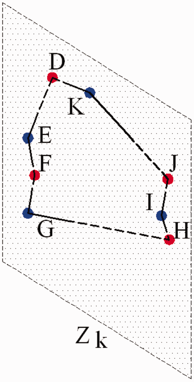
The cell division starts as the Lagrangian cells being cut into sub-elements by the two-dimensional faces of the Cartesian (Eulerian) cells. The surfaces of new sub-elements belong to either the original surfaces of the Lagrangian cells or the Cartesian surfaces cutting into. The boundaries of sub-surfaces are defined by the intersection points of all cut surfaces which are computed and saved whenever there is a relative motion of the two meshes. Figure 3 demonstrates a case of a tetrahedron being divided into three sub-elements by two background Cartesian surfaces.

Figure 3.

Cell division of a tetrahedron cell by two background Cartesian surfaces.

The basic rule for cell division to generate sub-elements is simple and it adds almost negligible computational overhead. However, some extreme cases may appear in the implementation and require special treatments. Figure 4 shows an example of such special cases. The tetrahedron OABC represents a typical Lagrangian solid cell for the computation of elastic stresses. The cell is cut by Cartesian surfaces X_i, $X_{i+1}$ , Y_j, and $Y_{j+1}$ of the background Eulerian framework. As the Lagrangian cells move, the relative locations of surfaces are changed and result in different divisions. The special case here assumes that the cell surface OAC coincide to the location of one Cartesian surface Z_k. In theory, its sub-surface DEFGHIJK from the cut stays on the surface Z_k. However, the sub-surface is described by all intersection points which are computed numerically as the tetrahedron moving through the background surfaces. The characteristics of numerical process inevitably lead to misalignment of these intersection points at the level of round-off error. The newly defined sub-surface will not be perfectly coincided to the location of Z_k or even perfectly flat. A possible scenario is shown in Figure 5, where some points (in red) are behind the surface Z_k and other points (in blue) are in front of of Z_k. The misalignment essentially defines some concave cells and leads to the invalidation of derivation and a failed computation. It is not hard to notice that the above scenario and anything similar only happen when a vertex of the tetrahedron cell is close enough to the background Cartesian surface. So, one remedy is to add a check process for all vertices before the cell division and prevent the situation in an ad hoc manner. ⁴³ It is noted that this challenge of misalignment does not appear in previous studies of two-dimensional configurations.^10,21,31,41 The reason is simply that two intersection points guarantee a straight line to define edges (of sub-elements) in a two-dimensional case but multiple intersection points will not numerically guarantee a flat surface to define sub-surfaces in a three-dimensional case.

Figure 4.

Demonstration of a tetrahedron OABC being cut by the background Cartesian surfaces X_i, $X_{i+1}$ , Y_j, and $Y_{j+1}$ , where the surface OAC is assumed to be parallel to a Cartesian surface Z_k, and the cut of surfaces creates a new sub-surface DEFGHIJK .

Figure 5.

A possible scenario for the sub-surface DEFGHIJK being misaligned with the background Cartesian surface Z_k: red points are behind Z_k and blue points are in front of Z_k.

Benchmark studies

Two benchmark cases were studied for the validation of different aspects in the development of the current algorithm: (1) a two-dimensional viscoelastic particle in shear flow is simulated to validate the treatment of solid in the unified formulation and its interaction with surrounding fluids; (2) the flow passing a rigid sphere, as a classical flow dynamics problem with embedded solid structure, to further validate the extension of the algorithm from two-dimensional to three-dimensional.

Viscoelastic particle in shear flow

To validate the accuracy of treating elastic stresses in the unified Eulerian framework and the associated fluid–solid interaction in the same framework, the algorithm is applied for the simulation of a two-dimensional floppy viscoelastic particle in shear flow (Figure 6). It is noted that the immersed boundary approach used here is fast and different from the algorithm in the original study of the same problem.^44,45

Figure 6.

Sketch of a viscoelastic particle in a shear flow.

Typically, the inertia term is neglected for creeping-flow problems where the Reynolds number, $\mathit{Re}=\rho \dot{\gamma }{a}^2/{\mu }_f$ , based on shear rate $\dot{\gamma }$ and particle radius a is very small. The governing equation becomes

$$\frac{\partial {\mathbf{u}}_m}{\partial t}=-\nabla p_m+\frac{1}{\mathit{Re}}{\nabla }^2{\mathbf{u}}_m+\nabla ·({\chi }_s{\mathit{\tau }}_s)$$

(22)

where the stress ${\mathit{\tau }}_s$ is based on the same neo-Hookean model in equation (14). Figure 6 shows the basic setup of the problem that a viscoelastic particle initially with circular shape is moving, deforming, and rotating under the interaction with the surrounding Couette flow. Three different types of motions, shown in Figure 7, are determined by the particleed initial aspect ratio ω₀ and capillary number $G=\dot{\gamma }{\mu }_f/{\mu }_s$ : tank-treading, swinging (trembling), and tumbling.

Figure 7.

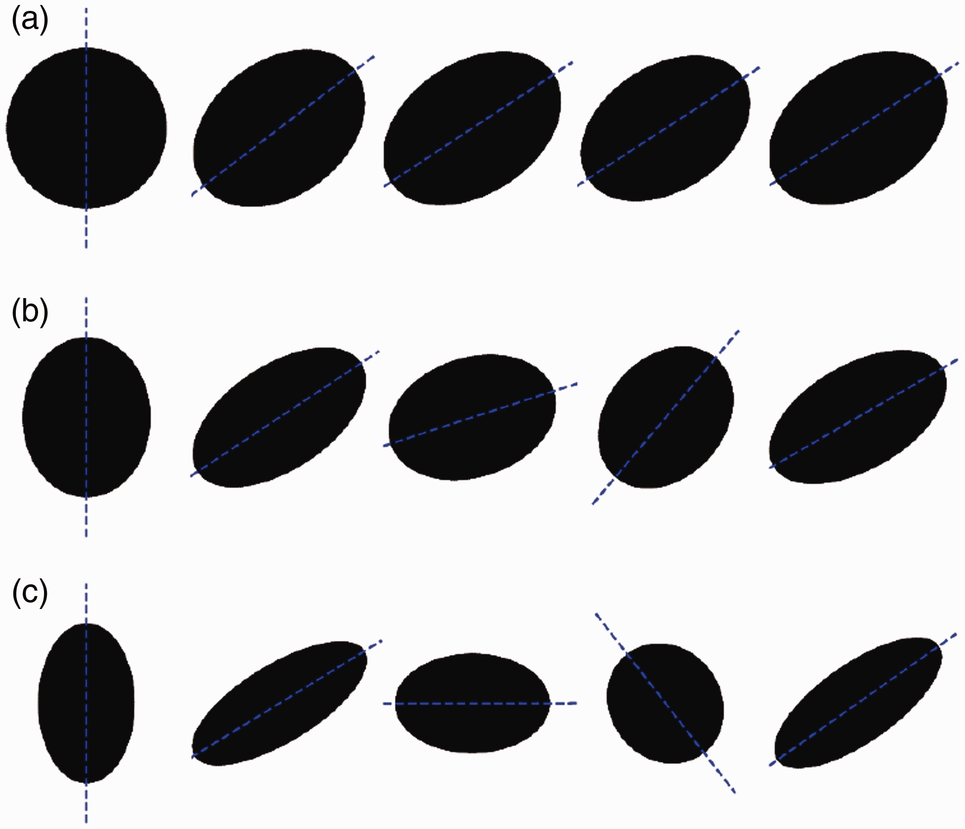
Different types of motion of viscoelastic particle in a shear flow: (a) tank-treading, (b) trembling, (c) tumbling.

The current immersed boundary approach was able to simulate all different types of motions. The computational domain is $[-2,2]\times [-2,2]$ with the mesh of 200 × 200. For a more quantitative benchmark, parametric study was performed for different aspect ratio and capillary number to find the boundary in parametric space to separate the region of trembling motion and the region of tumbling motion. As shown in Figure 8, the boundary computed by the current approach matches well with the study of others using a different approach. ⁴⁵

Figure 8.

Regions of trembling motion and tumbling motion for a two-dimensional viscoelastic particle in a shear flow: a comparison of our results to the results from literature ⁴⁵ using a different approach.

Incompressible flow passing a rigid sphere

An incompressible flow passing a stationary rigid sphere, as a classical benchmark case, has been investigated theoretically, numerically,^46,47 and experimentally.^48,49 This case was used to further validate the current approach of using a unified fluid–solid equation in a three-dimensional configuration which was not included in the first benchmark case. There are two reasons to consider only a rigid sphere in this validation: one is that the rigid sphere case is well studied and suitable for benchmark purpose, and the other is that the elastic formulation has already been validated in the first benchmark but the direct-forcing term (for rigid body and control gears) has not been validated yet.

In this study, the non-dimensional diameter of the sphere is D = 1, and the free stream velocity is $u_{\infty }=1$ . The dynamic viscosity of fluid μ_f is varied for different Reynolds number $R_e=\rho u_{\infty }D/{\mu }_f$ : R_e = 50, 100, 150, 200, 250, and 300, which are the same as the numbers used by Johnson and Patel. ⁴⁷ The computational domain is $[-10,10]\times [-4,4]\times [-4,4]$ with the mesh of $500\times 100\times 100$ . As shown in Figure 9, at low Reynolds numbers R_e = 50, 100, 150, and 200, the downstream flow is axisymmetric and different wake patterns are compared quantitatively between the simulations by the current algorithm and the study of Johnson and Patel. ⁴⁷ When Reynolds number increases to 250 and 300, the flow becomes asymmetric and a clear structure of hairpin vortex appears. Figure 10 compares the hairpin structure computed by Johnson and Patel ⁴⁷ and the current approach at Reynolds number 300. A more quantitative comparison is given in Figure 11, where the drag coefficient

$$C_d=\frac{F_d}{\frac{1}{2}\rho U_{\infty }^{2}D}$$

(23)

is computed for different Reynolds numbers. A good match is observed between our results and other numerical and experimental studies.^47,48

Figure 9.

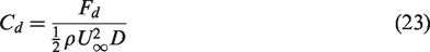
Comparison of the vorticity contours (ω_z) showing different wake patterns for the flow passing a sphere: (left) the numerical simulation by Johnson and Patel ⁴⁷ and (right) the current simulation using an immersed boundary approach with a unified formulation.

Figure 10.

Comparison of the flow structure of hairpin vortex from a flow passing a sphere at R_e = 300: (a) Johnson and Patel ⁴⁷ and (b) the current simulation.

Figure 11.

Comparison of the drag coefficient for a flow past a sphere with different Reynolds numbers.

Application on the simulation of a MAV with flexible wings

Established by the aforementioned benchmark cases, the current approach is ready for the simulation to study the aerodynamics of a MAV with flexible flapping wings, where the challenges of three-dimensionality, elastic structures, and direct-forcing controls all exist.

The computation domain is $-1<x<3,-1<y<1$ , and $0<z<2$ , with a mesh of $200\times 100\times 100$ . A uniform staggered mesh is used in an Eulerian framework, and quadratic tetrahedron cells are used for a Lagrangian mesh.

The wing model used in this simulation is based on the measurements from a wing of a toy MAV (by Interactive Toy Concepts Ltd). Figure 12 compares the original toy model to the numerical model with flapping motion. The lengths in the figure are non-dimensionalized by the length of the wingth leading edge. The green part of the numerical model moves passively and described by the elastic terms in the unified formulation, and the blue part of the model is prescribed by the direct-forcing terms either to control the flapping motion (the blue “lueonngor line) or to fix the wing structure to the body (the blue patch).

Figure 12.

Demonstration and comparison: (top) a toy MAV and its flexible wing; (bottom) the numerical model and the basic dynamics. In the numerical model, the green part is flexible with passive motion and the blue part is rigid with prescribed motion.

The flapping of wing is driven by the rotation of the blue “skeleton” line described by the flapping angle θ (marked in Figure 12) and the angular velocity $\omega =\dot{\theta }$

$$\theta =\frac{a}{L}\sin (2.0K\pi t)+{\theta }_0$$

(24a)

$$\omega =\frac{2.0aK\pi }{L}\cos (2.0K\pi t)$$

(24b)

where a = 0.1, $K=1.0/\pi ,L=18/(19.5\pi )$ , and ${\theta }_0=10.5°$ . The parameters were chosen to match with the realistic data of the toy as close as possible. In the study, two cases are simulated to understand the impact from two different angles of attack, $\alpha =0°$ and $\alpha =14°$ .

As shown in Figure 13, the wing deformation of the case with angle of attack $\alpha =0°$ is larger in both the deformation amplitude and the size of area with obvious deformation. For more quantitative comparison, the deformation is painted on wing surfaces by contours measured by the distance between points on the deformed wing surface and their projection on an imaginary rigid wing surface under the same motion. In fact, this larger deformation of the flexible wing shown in the case of $\alpha =0°$ may help to limit the width of vortex structures shedding as shown in Figure 14. It is also shown in Figure 14 that higher value of streamwise vorticity (marked in red), ${\omega }_x\ge 1$ , is being sustained further downstream in wake structures when the angle of attack is higher, as an indication of generally stronger shedding vortices in the case with higher angle of attack.

Figure 13.

Wing deformations when flapping with the angle of attack $\alpha =0^{°}$ (top row) and $\alpha ={14}^{°}$ (bottom row) at different phases of a period: (a) t = 0, (b) t = T/4, (c) t = T/2, and (d) t = 3T/4. The deformation is also highlighted by the contours on wing surfaces, which are measured by the distance deviated from the rigid wing under the same motion.

Figure 14.

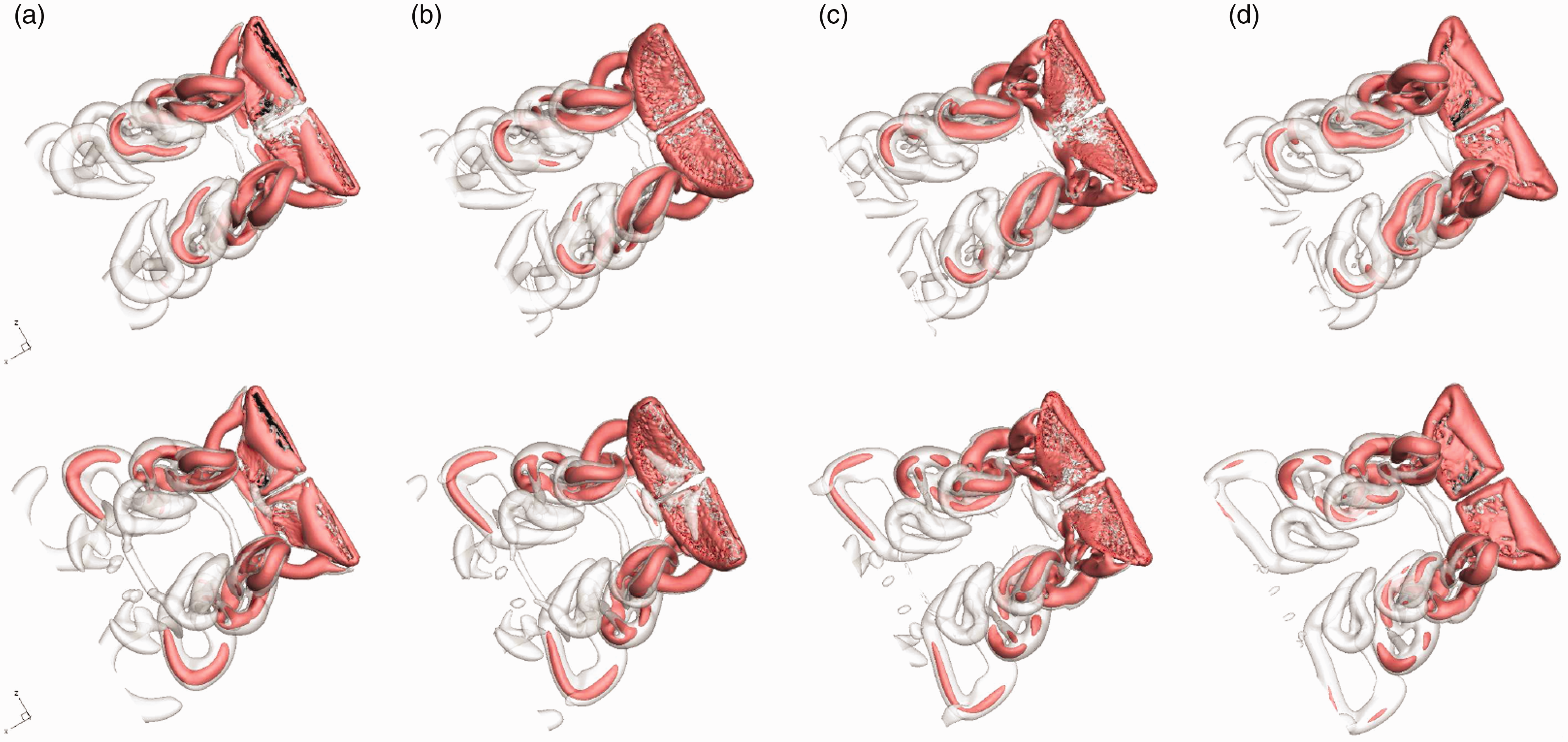
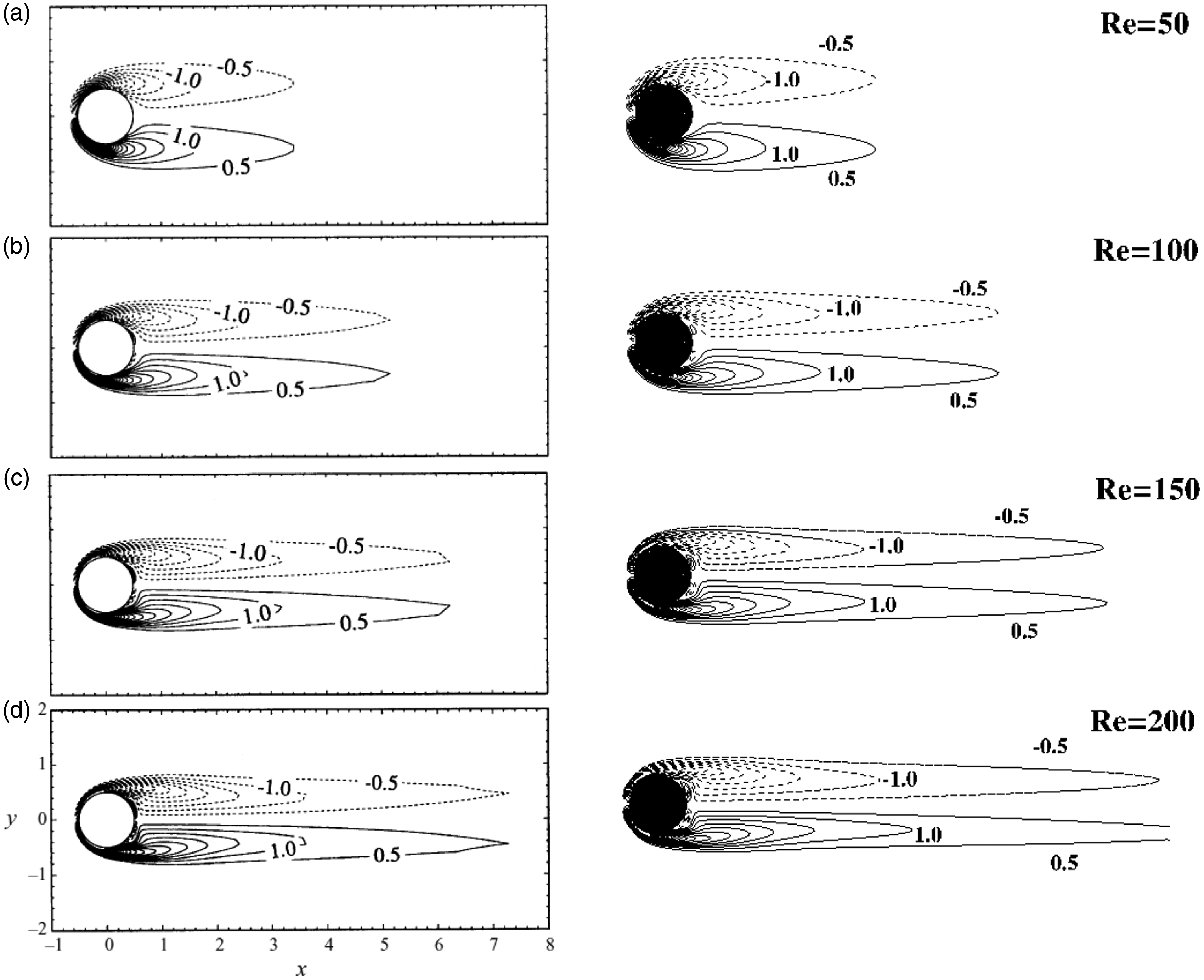
Vortex structures of the wake flows when the wing flapping with the angle of attack $\alpha =0^{°}$ (top row) and $\alpha ={14}^{°}$ (bottom row) at different phases of a period: (a) t = 0, (b) t = T/4, (c) t = T/2, and (d) t = 3T/4. The vortex structure is shown by the iso-surface of Q criteria and highlighted by the streamwise vorticity ${\omega }_x\ge 1$ .

Figure 15 compares the overall aerodynamic performance of these two cases. It is not surprising to see the non-dimensional lift increases with the increase of angle of attack, with the averaged non-dimensional lift ${\overline{F}}_L=3.92\times {10}^{-2}$ for $\alpha =0°$ and ${\overline{F}}_L=4.58\times {10}^{-2}$ for $\alpha =14°$ . The effect on drag is, however, more complicated. For the case of $\alpha =14°$ , though the shedding vortex is stronger, the resulted thrust is actually smaller as the vortex structures are diverted sideward. As the result, the case of $\alpha =0°$ actually achieves a thrust with an averaged non-dimensional drag ${\overline{F}}_D=-1.44\times {10}^{-2}$ (the negative sign indicates a thrust), while the case of $\alpha =14°$ stays in the drag region with an averaged non-dimensional drag ${\overline{F}}_D=7.52\times {10}^{-3}$ under current control parameters.

Figure 15.

Time history of the (a) lift and (b) drag for the flexible wing flapping at different angle of attack $\alpha =0^{°}$ and $\alpha ={14}^{°}$ .

Conclusions

In this study, a strongly coupled three-dimensional algorithm for FSI is constructed through a monolithic immersed boundary method. The motions of flows and structures as well as its interaction are simulated under a unified Eulerian framework, while the location of structure is tracked accurately by a Lagrangian mesh. The interpretation and projection between the Eulerian and Lagrangian frameworks are calculated through a cell division technique and Gauss quadrature. It should be noted that the interpretation and projection between the Lagrangian and Eulerian frameworks are meant for the evaluation of solid elastic stress, and the time advancement for both fluid and solid is performed in an Eulerian framework (i.e. the unified governing equation). It is intrinsically a monolithic immersed boundary algorithm for fluid–solid interactions in an Eulerian description.

The monolithic FSI algorithm was validated by comparing the simulation results with other numerical simulations and experimental measurements in literature using two classical cases to cover two- and three-dimensional configurations and rigid and flexible structures: the flow passing a three-dimensional rigid stationary sphere and a two-dimensional floppy viscoelastic particle in a shear flow. The qualitative and quantitative comparisons agree well with the existing literature in both cases.

The monolithic FSI algorithm was then used to study three-dimensional flexible flapping wings with different kinematics and parameters in a forward flight. The simulations at an angle of attack $\alpha =0°$ and $\alpha =14°$ showed the impact from the angle of attack to wing deformation, wake vortex structures, and eventually aerodynamic performances of a flexible flapping wing in forward flight. It is shown that the vortex street in wake tends to spread spanwise at larger angle of attack while the strength increases slightly. Further investigation shows that, at lower angle of attack, the larger deformation of flexible wings helps to align the vortex street downstream and reduce the wake spreading, and therefore increase the vortex-generated thrust. Overall, the case with angle of attack $\alpha =0°$ provides more thrust, and the case of larger angle of attack at $\alpha =14°$ provides more lift.