Sage Journals: Discover world-class research

Abstract

The demand for micro-air vehicles is increasing as well as their potential missions. Whether for discretion in military operations or noise pollution in civilian use, the improvement of aerodynamic and acoustic performance of micro-air vehicles propeller is a goal to achieve. Micro- and nano-air vehicles operate at Reynolds numbers ranging from 10³ to 10⁵. In these conditions, the aerodynamic performance of conventional fixed and rotary wings concepts drastically decreases due to the increased importance of flow viscous forces that tend to increase drag and promote flow separation, which leads to reduced efficiency and reduced maximum achievable lift. Reduced efficiency and lift result in low endurance and limited payloads. The numerical simulation is a potential solution to better understand such low Reynolds number flows and to increase the micro-air vehicles’ performance. In this paper, it is proposed to review some challenges related to micro-air vehicles by using a Lattice-Boltzmann method. The method is first briefly presented, to point out its strengths and weaknesses. Lattice-Boltzmann method is then applied to three different applications: a DNS of a single blade rotor, a large eddy simulation of a rotor operating in-ground effect and a large eddy simulation of a rotor optimised for acoustic performance. A comparison with reference data (Reynolds Averaged Navier-Stokes, DNS or experimental data) is systematically done to assess the accuracy of lattice-Boltzmann method-based predictions. The analysis of results demonstrates that lattice-Boltzmann method has a good potential to predict the mean aerodynamic performance (torque and thrust) if the grid resolution is chosen adequately (which is not always possible due to limited computational resources). A study of the turbulent flow is conducted for each application in order to highlight some of the physical flow phenomena that take place in such rotors. Different designs are also investigated, showing that potential improvements are still possible in terms of aerodynamic and aero-acoustic performance of low-Reynolds rotors.

Keywords

Lattice-Boltzmann method micro-air vehicles aerodynamics aero-acoustics

Introduction

Numerical simulation, supported by high-performance computing (HPC) and experimental validation, led to major breakthroughs in our knowledge of complex physical phenomena and our capability to design innovative technologies. To go beyond the current state of the art, there is still a need to improve our aptitude to deal with complex flow physics, including aerodynamics, aero-acoustics or fluid/structure interactions. Such capabilities are mandatory to address ambitious targets, such as earth exploration but also the investigations beyond the limit of our planet. Together with the advent of micro-technologies, micro-air vehicles (MAVs) recently appeared as a relevant solution for missions of observation and surveillance. MAVs with enhanced endurance and ability to operate in constrained environments would considerably decrease surveillance costs while preserving safety of the operators in many civilian and military applications. They can also be used in an environment where the presence of humans is not yet possible. However, because of their small dimensions and the intrinsically low Reynolds numbers at which they operate, as well as the difficulty to optimise aerodynamic performance for both forward and hovering flight, current MAVs exhibit relatively low endurance (typically between 15 and 25 min in hover).

Low-to-moderate Reynolds number flows, typical of MAVs ( $R e \approx 10^{3} - 10^{5}$ ), tend to promote flow separations (that decrease efficiency and lift), which are difficult to predict with classical computational fluid dynamics methods, based on a Reynolds Averaged Navier-Stokes (RANS) approach (where all scales of turbulence are modelled). With the increase in computing power, large eddy simulation (LES) emerges as a promising technique to improve the reliability of flow solver predictions.¹ Several works have already shown that LES leads to significant improvements both in the understanding of flow physics and the performance predictions of rotors.² Usually, LES is based on the resolution of the filtered Navier-Stokes equations. While effective, this method requires the use of artificial dissipation which limits its accuracy (e.g. transport of turbulence on a long distance, noise predictions, etc.). Lattice-Boltzmann method (LBM) is a recent and (more and more) popular alternative to such Navier-Stokes flow solvers.³ Instead of directly solving the Navier-Stokes equations, this method tackles the Boltzmann equation, a statistical equation for the kinetics of gas molecules. Thus, the primitive variables of the LBM represent the statistical particle probability distribution function, to which the usual macroscopic variables, such as pressure and velocity, relate as velocity moments, or as observables in the sense of statistical mechanics. The particle distribution is a continuous quantity: in contrary to popular believe, the LBM is a continuum method and not a discrete particle approach. Indeed, the method offers an Eulerian view of the flow and is mesh based.

To illustrate the advantages and drawbacks of LBM, three applications have been selected in line with MAV challenges: a Direct Numerical Simulation (DNS) of a single blade rotor at low Reynolds number, a LES of a rotor operating in-ground effect and a LES of a rotor optimised for acoustic performance.

Description of the LBM

The LBM considers the discrete Boltzmann equation, a statistical equation for the kinetics of gas molecules, instead of solving directly the Navier-Stokes equations. The primitive variables of the LBM represent the statistical particle probability distribution function, to which the usual macroscopic variables, such as pressure and velocity, relate as velocity moments. In that regard, the particle distribution function is a continuous quantity (and not on a discrete particle approach). Beyond its computational performance, the main advantage of LBM is that the method is stable without artificial dissipation, which makes the method equivalent to solve the Navier-Stokes equations with a high-order numerical scheme. Its drawback is that it requires the use of Cartesian grids, which dramatically increase the number of grid points necessary to compute the flow close to walls. As detailed in Lallemand and Luo³ and D’Humieres et al.,⁴ the governing equations of LBM consider the probability $f_{i} (x, t)$ to have a set of particles at location x and time t, with a velocity c_i

f_{i} (x + c_{i} δ t, t + δ t) = f_{i} (x, t) + Ω_{i j} (x, t)

(1)

for

[0 < i, j < N]

, where c_i is a discrete velocity of a set of N velocities and Ω _ij is an operator representing the internal collisions of pairs of particles. For the present 3D problems, the kinetic scheme is based on the D3Q27 set of velocities (27 velocities, so equation (1) is solved 27 times, for each velocity c_i). This kinetic scheme ensures the conservation of mass and momentum, which are related to the population of particles, f_i, as

ρ = \sum_{i = 1}^{N} f_{i}

and

ρ u = \sum_{i = 1}^{N} f_{i} c_{i}

. The numerical method is divided into two steps: a collision step (during which the collision model is used to relax the particle populations towards their equilibrium) and a streaming step (during which the new populations of particles are transported to neighbouring sites with the velocity c_i). Such an approach is of second order both for the spatial discretisation and time integration.

The collision operator is represented by a single relaxation time model, and a regularisation technique is applied to increase the stability and accuracy of the method.^5,6 The regularisation step can be seen as an explicit filtering step (that is applied at each time step). Depending on the target in terms of Reynolds number, the turbulence can be fully simulated (DNS) (e.g. for the application to the single blade rotor at Reynolds number 10³) or only the largest scale can be simulated while the smallest one are filtered (LES).⁷ Due to the filtering provided by the regularisation step, the use of subgrid scale model is not mandatory (however, SGS models as the Smagorinsky model are available). The LBM equations are solved using the open source software Palabos (www.Palabos.org), developed by the University of Geneva.

The boundary conditions on the external faces of the computational domain are of Neumann type with zero velocity and pressure gradients. With this set of boundary conditions, the flow inside the computational box is fully driven by the rotor, and hence it helps to reduce the time needed to converge the flow inside the computational box. Sponge layers are imposed on each face to limit spurious reflections of acoustic waves, as proposed in Bodoni.⁸ Such sponge layers rely on a progressive increase of the flow viscosity in order to damp the pressure and velocity fluctuations close to the boundary conditions. The movement of rotating blades is represented in the computational grid through an immersed boundary approach.⁹ A wall model can be used to improve the description of the boundary layers.¹⁰ However, due to the low number of grid points generally used in the boundary layer (less than 10 for the applications reported in this paper), the numerical predictions close to the wall should be considered with caution.

Single-bladed rotor at low-Reynolds number

The first application deals with the development of bio-inspired nano-flying robots. At very small scales, the observation of nature suggests that flapping wings may be a relevant solution to perform both hovering and forward flight with enhanced manoeuvrability. Although there is no compelling evidence that flapping wings are more aerodynamically efficient (or alternatively more aeroacoustically efficient) than other hovering capable concepts, in particular rotating wings, flapping wings have gained considerable attention due to the unique flow features upon which it relies. These include the development of a large-scale leading edge vortex (LEV), wing–wake interactions and other unconventional mechanisms such as clap-and-fling, depending on the precise kinematics of the flapping wing (see Shyy et al.,¹¹ for a review). Among these mechanisms, the development of an intense conical LEV has proven to be the predominant mechanism at play for the generation of strong aerodynamic forces. The dynamics of the LEV can be investigated by looking at a single stroke of the whole flapping cycle. Note that a flapping cycle can essentially be decomposed into two revolving phases – namely the downstroke and upstroke phases – and two rotating phases – namely the pronation and supination phases. In this section, a direct numerical simulation of the flow is performed past a single stroke of the flapping cycle, which is here modelled by a wing revolving at constant speed about its root.

The main characteristics of the blade are summarised in Table 1. The wing has a rectangular planform with an aspect ratio of 4. It revolves at constant speed (impulsively started) about its root through 180°. The blade angle is set to 45°. The Reynolds number based on the revolving speed and the wing chord at the tip is 10³. Figure 1 shows the instantaneous lift coefficient C_L as a function of the revolving angle $ϕ$ , defined as

C_{L} = \frac{L (ϕ)}{\frac{1}{2} ρ {(Ω . R_{p})}^{2} . S}

(2)

with L the lift, ρ the density, R_p the radius at the pressure centre point (evaluated at

R_{p} = 0.0231

m) and S the surface of the blade.

Figure 1.

Comparison of lift coefficient between DNS–LBM and DNS results obtained by Mengaldo et al.¹² and Jardin and David.¹³

Table 1.

Main parameters of the single blade rotor.

Number of blades	1
Rotation rate, Ω	37.5 rad.s^–1
Rotor tip speed	1.5 m.s^–1
Rotor blade chord, C	0.01 m
Rotor radius, R	0.04 m
Reynolds number, Re	10 × 10³

Results are compared with those reported in Mengaldo et al.¹² (DNS with an immersed boundary Lattice Green Function Method^14,15) and Jardin and David¹³ (DNS obtained with the commercial STAR-CCM+ software). It is shown that the results obtained from the present DNS–LBM approach match those obtained with other well-validated methods within reasonable accuracy (less than 3%). Three grids have been designed with resolution $Δ x = 0.015 C, Δ x = 0.012 C, Δ x = 0.011 C$ (with C the blade chord), respectively. Converged lift is achieved for resolution finer or equal to $Δ x = 0.012 C$ . Indeed, while approaches by Mengaldo et al.¹² and Jardin and David¹³ demonstrate mesh independency for cell sizes on the order of $0.015 C$ , the present LBM approach requires space resolution on the order of $0.012 C$ , which demonstrates the good accuracy of the immersed boundary method used in the LBM code.

Present results show that the revolving wing produces high levels of lift (considering the Reynolds number at which it operates) immediately after the impulsive start. In addition, lift remains at high levels during the whole revolving motion. This is fundamentally different to what is observed on a two-dimensional airfoil where the lift first reaches high levels but then drops together with the separation of the LEV. Figure 2 shows that sustained lift is correlated with the development of a stable LEV on the upper surface of the wing. The LEV develops during the initial stages of the revolving motion but rapidly reaches a stable state, i.e. it does not shed into the wake, hence generating high aerodynamic forces. Recent studies suggest that LEV stability is promoted by rotational effects^16–18 and is therefore inherent to low aspect ratio of the revolving and rotating wings. Present results further show that the conical LEV bursts into small-scale structures at the wing tip, in agreement with experimental observations,^19,20 highlighting the capability of the present DNS–LBM approach to track the onset of chaotic/turbulent flow. Such capability is further investigated in the next sections, at higher Reynolds numbers.

Figure 2.

Iso-surface of Q criterion obtained from DNS–LBM simulations at different instants of time that describe half a rotation of the blade.

Two-bladed rotor in-ground effect

This application targets the prediction of the turbulent flow produced by the MAV rotor interacting with the ground,²¹ at moderate Reynolds number, $R e \approx 10^{5}$ . The main parameters of the configuration are summed up in Table 2. The rotor is composed of two untwisted flat plates, with a radius R = 0.125 m. The chord of the blade C is set to 0.025 m. The pitch angle of the blade θ is set to 15°. The rotor is located at two radii from the ground, corresponding to $z / R = 2.0$ (z = 0 corresponds to the ground and $z / R = 2.0$ corresponds to the rotor). An overview of the flow produced by such a configuration is shown in Figure 3. The wake generated by the rotor impacts the ground and is progressively deviated towards the outside part of the domain. A boundary layer then develops at the ground level. Such a flow impacts the operability of MAVs using propellers²² and can limit the mission that can be achieved, especially in highly confined environment (exploration of cave or buildings). An accurate description of the rotor wake in-ground interaction requires the use of complex methods based on overset grids and vortex tracking algorithms.²³

Figure 3.

Instantaneous flow field obtained with LES–LBM.

Table 2.

Main parameters of the two-bladed rotor in-ground interaction.

Number of blades	2
Rotation rate, Ω	414.69 rad.s^–1
Rotor tip speed	51.8 m.s^–1
Rotor blade chord, C	0.025 m
Rotor radius, R	0.125 m
Reynolds number, Re	0.86 × 10⁵

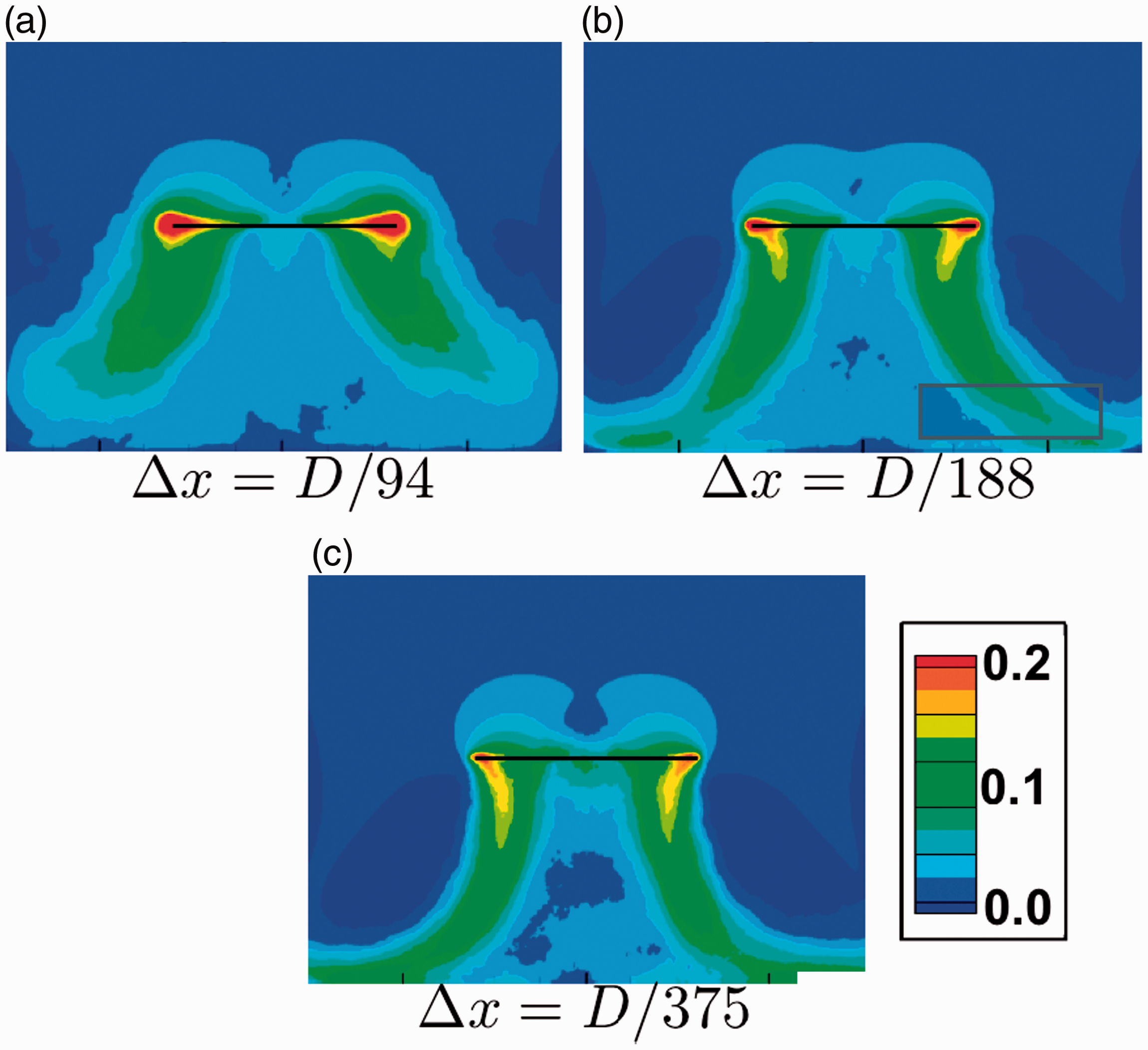
The main objective of this application is to validate the capability of LES–LBM to reproduce the flow generated by such in-ground effect, by comparing with the experimental data. To study the sensitivity of the solution to the grid, three meshes are used to perform the numerical simulations: for each grid, the resolution is increased by a factor of 2 compared to the previous grid. The resolutions compared to the rotor chord are, respectively, $Δ x / C = 0.100$ (grid 0), $Δ x / C = 0.050$ (grid 1) and $Δ x / C = 0.025$ (grid 2). The rotor diameter (from the root to the tip) is described, respectively, by 94 points (grid 0), 188 points (grid 1) and 375 points (grid 2). The total number of points is, respectively, $13 \times 10^{6}, 105 \times 10^{6}$ and $830 \times 10^{6}$ for grid 0, grid 1 and grid 2. A complete rotation of the rotor requires, respectively, $3 \times 10^{3}, 6 \times 10^{3}$ and $12 \times 10^{3}$ time steps for grid 0, grid 1 and grid 2.

A comparison of the time-averaged flow field obtained with the three grids is shown in Figure 4. Regarding the convergence of the flow close to the ground, the numerical simulation on grid 0 is not able to reproduce the interaction of the rotor wake with the ground. The main reason is due to the under-prediction of the rotor thrust (as reported in Gourdain et al.²¹), which results in a lower velocity at the rotor outlet and a dissipation of the wake before it reaches the ground. Results on grids 1 and 2 are in reasonably good agreement, but discrepancies are observed in the rotor wake (where the peaks of velocity are under-estimated with grid 1) and close to the ground (where the velocity in the ground boundary layers is under-estimated with grid 1). This qualitative comparison shows that the obtention of grid-independent results remains a difficult task with pure Cartesian grids (the use of a hierarchical grid refinement, as considered for the third application, could help to overcome this limitation). For this reason, only the results on grid 2 are compared with the experimental data.

Figure 4.

Time-averaged flow field coloured with normalised velocity $V / (Ω . R)$ : (a) grid 0, (b) grid 1 and (c) grid 2.

Experimental data from Jardin et al.²⁴ are compared with numerical predictions obtained on grid 2. Experimental measurements rely on the particle image velocimetry (PIV) technique. The PIV system consists of a 2 × 200 mJ DualPower Bernoulli laser to which two FlowSense EO 16M cameras are synchronised, using DantecStudio commercial software. The comparison is shown in Figure 5(a) (at two heights from the ground) and Figure 5(b) (at two radial locations). This comparison shows that LES–LBM correctly reproduces the time-averaged flow, in the vicinity of the rotor wake ( $z / R = 1.5$ ). The discrepancy with measurements, close to the rotation axis ( $x / R = 0.0$ ), is mainly related to the presence of the motor that is excluded from the numerical simulations. At $z / R = 0.5$ , approaching the ground, LES–LBM under-predicts the peak velocity by 7%, but the thickness of the rotor wake is well predicted, included far from the rotor.

Figure 5.

Comparison between experimental data and LES–LBM of time-averaged velocity signals: (a) $V = f (x / R)$ and (b) $V = f (z / R)$ .

The interaction between the rotor wake and the ground drives the development of a ground boundary layer. The velocity magnitude is shown in Figure 5(b) at two locations, $x / R = 1.0$ (where the rotor wake impacts the ground) and $x / R = 2.0$ . LES–LBM is in good agreement with measurements, especially close to the ground. At $x / R = 1.0$ , LES–LBM under-predicts the peak of velocity by less than 5%, and the location of the velocity peak is shifted from $z / R = 0.55$ to $z / R = 0.60$ , compared to experimental data. At $x / R = 2.0$ , the thickness of the shear layer is well reproduced by the LES–LBM approach and the peak of velocity is also slightly under-predicted by 7%. This quantitative comparison demonstrates that LES–LBM on grid 2 is able to reproduce the complex flow field generated by the interaction between a rotor and the ground.

To reduce the influence of the wake on the ground, a ducted rotor is compared with the initial free rotor. The immersed boundary approach is well suited to such an approach, as it allows continuing the numerical simulation by simply adding a shroud to the rotor, which avoid complex remeshing operations (which are often done manually).

Shrouded rotors usually generate more thrust than equivalent free rotors at a given rotation speed.²⁵ Indeed, the presence of a shroud contributes, at a given thrust, to reduce the velocity at the ground level since the rotation speed of the rotor can be reduced compared to unshrouded rotors. In this work, the rotational speed of the shrouded-rotor configuration can be reduced by 27%, with respect to the free rotor configuration, to provide similar total thrust. This reduction in rotation speed leads to a direct reduction of the flow velocity at the ground level. In addition, another effect of the shroud is to expand the rotor jet (through a diverging nozzle), which further contributes to decrease the downward velocity of the rotor wake. All this is conducive to weaker interactions between the rotor and the ground. The velocity flow field generated by ducted and free rotor configurations are compared at a constant thrust in Figure 6. At $x / R = 1.0$ , the duct is responsible for a shift of the velocity peak from $z / R = 0.6$ (free rotor) to $z / R = 1.0$ (ducted rotor). At the ground level, the velocity is reduced by 20%, compared to the free rotor. This behaviour is also well highlighted in Figure 7 that shows the time evolution of the velocity fluctuations at $z / R = 1.0$ (mid-distance between the ground and the rotor). A low-frequency oscillation of the rotor wake is observed only for the free rotor configuration (represented by the dashed line). This low-frequency phenomenon is suppressed in the case of a ducted rotor. Indeed, this work also indicates that the behaviour of the flow at the ground level is more stable in the case of a ducted rotor than in the case of a free rotor.

Figure 6

Comparison between a ducted rotor and a free rotor at constant thrust, interacting with the ground: time-averaged velocity flow field $V / (Ω . R)$ .

Figure 7.

Velocity fluctuation $u' / (Ω . R)$ flow field at $z / R = 1.0$ , with respect to normalised time: (a) free rotor and (b) ducted rotor. The dashed dot line indicates the location of velocity peaks and the dashed line shows the low frequency phenomenon in the case of the free rotor.

The conclusion of this second application is that LES–LBM successfully reproduces the flow generated by the rotor/ground interaction (which is validated by a comparison with experimental measurements). The use of immersed boundaries is also a very convenient way to study different geometries for the same configuration, avoiding the use of a costly remeshing step. However, the near wall flow has not yet been validated, due to unsufficient grid resolution and a lack of experimental data in the vicinity of the rotor.

Three-bladed rotor optimised for aero-acoustic performance

Whether for discretion in military operations or noise pollution in civilian use, noise reduction of MAV is a goal to achieve. Aeroacoustic research has long been focusing on full-scale rotorcrafts. At MAV scales, however, the quantification of the numerous sources of noise is not straightforward, as a consequence of the relatively low Reynolds number that ranges typically from 10³ to 10⁵. Reducing the noise generated aerodynamically in this domain then remains an open topic. This part of the work deals with the numerical simulations performed through unsteady Reynolds-Averaged Navier-Stokes (URANS) and LES–LBM to study the flow phenomena that are responsible for the noise generation of a rotor in hover.

URANS

LES–LBM predictions are compared in this section with those provided by an URANS approach. The three-dimensional URANS equations are solved using a finite volume approach, by means of Star-CCM+ commercial code. The computational domain is discretised using polyhedral cells. The boundary conditions upstream and downstream the rotor are implemented as pressure conditions, while the periphery of the domain is treated as a slip wall. The blades are modelled as non-slip surfaces. Both spatial and temporal discretisations are achieved using second-order schemes. Momentum and continuity equations are solved in an uncoupled manner using a predictor–corrector approach. Specifically, a colocated variable arrangement and a Rhie-and-Chow-type pressure–velocity coupling combined with a SIMPLE-type algorithm are used.^26,27 A $k - ϵ$ model is employed for turbulence closure with maximum y⁺ values below 1 (boundary layers are assumed fully turbulent).

Geometry and grid convergence study

The test case is a three-bladed rotor, designed to reduce acoustic emissions. The design is yielded from a low-cost numerical tool developed at ISAE-Supaero based on blade element and momentum theory (BEMT)²⁸ for the aerodynamic prediction and formulation of the Ffowcs-Williams and Hawkings equation as expressed by Farassat²⁹ coupled with broadband noise models for the acoustic prediction. The distributions of lift and drag are estimated from the local lift and drag coefficients on 2D sections. The estimation of sectional aerodynamic performance relies on a low-fidelity approach, which considers Euler equations along a streamline coupled with an integral boundary layer formulation.³⁰ Such an approach demonstrated a good accuracy for low Reynolds number flows. More information about the design tool are available in Serre et al.³¹ The main characteristics of the rotor obtained with this design technique are indicated in Table 3. The airfoil section is a Gottingen 265, which is well adapted to low Reynolds number flows (thin and cambered profile).

Table 3.

Main parameters related to the three-bladed rotor.

Number of blades	3
Rotation rate, Ω	518.36 rad.s^–1
Rotor tip speed	45.4 m.s^–1
Rotor blade chord, C	0.024 m
Rotor radius, R	0.088 m
Reynolds number, Re	0.72 × 10⁵

Three grids are designed, which all match wall-model LES requirements: the dimension of the first cell in the direction normal to the wall is, respectively, set to 480 μm, 355μm and 240 μm (which corresponds to $\bar{y^{+}} \approx 35, \bar{y^{+}} \approx 25$ and $\bar{y^{+}} \approx 15$ ) for grid 0, grid 1 and grid 2. The discretisations of the airfoil are thus, respectively, $Δ x = 0.020 \times C$ (grid 0), $Δ x = 0.015 \times C$ (grid 1) and $Δ x = 0.010 \times C$ (grid 2), with C the mean chord of the profile. The radial direction (from the root to the tip) is discretised with 183 points, 251 points and 366 points, respectively. To reduce the number of grid points, a hierarchical grid refinement approach is used with seven grid levels (a grid level corresponds to a constant resolution part of the grid). The total number of points are, respectively, $23 \times 10^{6}, 153 \times 10^{6}$ and $179 \times 10^{6}$ for grid 0, grid 1 and grid 2. A full rotation of the rotor is discretised with, respectively, $11.6 \times 10^{3}, 16.0 \times 10^{3}$ and $23.2 \times 10^{3}$ time steps for grid 0, grid 1 and grid 2. The grid parameters for both URANS and LES are summed up in Table 4.

Table 4.

Main grid parameters for URANS and LES

	$Δ x / y^{+}$	$y^{+}$	$Δ z / y^{+}$	$Δ x / C$
URANS	20	1	20	0.022
LES–LBM, grid 0	1	35	1	0.020
LES–LBM, grid 1	1	25	1	0.015
LES–LBM, grid 2	1	15	1	0.010

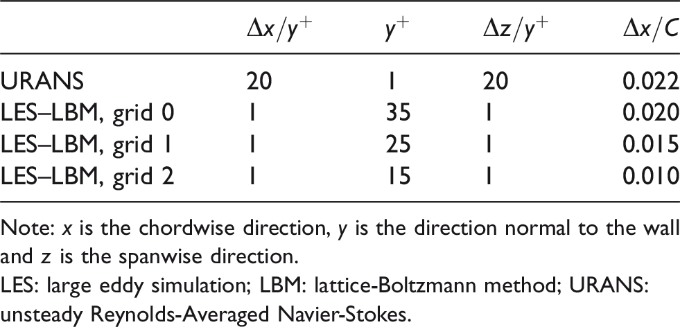
Note: x is the chordwise direction, y is the direction normal to the wall and z is the spanwise direction.

LES: large eddy simulation; LBM: lattice-Boltzmann method; URANS: unsteady Reynolds-Averaged Navier-Stokes.

The influence of mesh resolution is observed on the torque coefficient, defined as

C_{Q} = \frac{Q}{\frac{1}{2} ρ {(Ω . R)}^{2} π R^{3}}

(3)

with Q the torque. The results are shown in Figure 8. With all grid resolutions, the convergence of the torque coefficient is achieved after four rotor rotations. However, the torque coefficient is under-predicted by 10% with grid 0 compared to grid 2, and by 1% with grid 1 compared to grid 2. Despite the moderately good quality of the grid in the vicinity of the wall, the torque coefficient is not sensitive to the grid resolution when considering a resolution higher or equal to

Δ x / C = 0.015

, which is compatible with the results discussed for grid convergence study in previous sections. Only data obtained with grid 1, for which torque and thrust coefficients are converged, are analysed in the rest of the paper.

Figure 8.

Comparison of global performance: (a) thrust coefficient C_T and (b) torque coefficient C_Q.

Comparison with measurements

Three sets of data are compared with measurements: LES–LBM, URANS and BEMT (as used for the design step). Only the global aerodynamic forces are measured with a five-component balance. Indeed, the comparison between experimental and numerical predictions is done only for the torque and thrust coefficients, C_Q and C_T, defined as

C_{T} = \frac{T}{\frac{1}{2} ρ {(Ω . R)}^{2} π R^{2}}

(4)

with T the rotor thrust. These coefficients are shown in Figure 9. To check the dependency of the performance curve to rotation speed, another operating point at

Ω = 314.16 rad {.s}^{- 1}

(3000 r/min) has been simulated both with URANS and LES–LBM. At 3000 r/min, the accuracy of LES–LBM on thrust is very good (about 1%). Both URANS and BEMT over-predict the thrust coefficient by 15%.

Figure 9.

Comparison of global performance: (a) thrust coefficient C_T and (b) torque coefficient C_Q.

When considering the torque coefficient, the order of the methods regarding their accuracy is inverted: LES–LBM, URANS and BEMT over-predict torque by 50%, 40% and 21%, respectively. At 4950 r/min, similar conclusions can be drawn: the thrust coefficient is under-predicted by 2.5% with LES–LBM and over-predicted by 14% and 17% by URANS and BEMT, respectively. For the torque, LES–LBM, URANS and BEMT over-predict by 29%, 23% and 12%, respectively. It is unclear why three very different numerical methods over-predict the torque (especially the BEMT which neglect 3D effects and predicts fully attached boundary layers). Unfortunately, due to the lack of experimental data, it is not possible at the moment to identify the origin of such discrepancies.

The local thrust coefficient is plotted in Figure 10 for the three methods. As already shown, BEMT predicts the higher thrust coefficient and LES–LBM the lowest one. From the root to $r / R = 0.4$ , the three methods give the same local thrust coefficient. Then, both URANS and LES–LBM predict the same evolution until $r / R = 0.75$ , while BEMT already predicts a higher value. All methods show a peak for the thrust coefficient at $r / R = 0.82$ (URANS, LES–LBM) or 0.83 (BEMT). However, the values of C_T at the peak are different: C_T=0.19 (LES–LBM), 0.22(URANS) and 0.265 (BEMT). Beyond $r / R = 0.85$ , the value of C_T decreases rapidly. Actually, the main conclusion is that the three numerical methods agree reasonably well on a large part of the rotor span, but predict very different behaviour close to the tip, due to 3D flow effects.

Figure 10.

Comparison of local thrust coefficient, along the rotor span.

Analysis of the blade vortex interaction

One of the dominant sources of noise in the present rotor comes from the ingestion of turbulence by the leading edge of the rotor blades.^31,32 Figure 11 shows an instantaneous iso-surface of Q criterion, coloured by the pressure coefficient $- C_{p}$

- C_{p} = \frac{(p - p_{0})}{\frac{1}{2} ρ {(Ω . R)}^{2}}

(5)

Figure 11.

Instantaneous iso-surface of Q-criterion coloured by the pressure coefficient – Cp (LES–LBM data).

Three different vortices are generated close to the rotor tip: one starts at the leading edge, one comes from the pressure side and one begins at mid-chord. The breakdown of these three vortices starts close to the trailing edge, due to the recompression. These vortices merge also with the vortex due to the separation of the suction side boundary layer, close to the tip. The mixing process between the different vortices produces turbulence that impacts the following blade (located on the left part of the picture in Figure 11).

The numerical data obtained with URANS and LES–LBM are analysed for the reference configuration, for the rotation speed $Ω = 518.36 rad {.s}^{- 1}$ (4950 r/min). The flow field coloured with the normalised streamwise component of the velocity $V_{z} / (Ω . R)$ is shown in Figure 12, at the altitude $z / R = 0$ , that corresponds to a plane that intersects the blade close to the rotor trailing edge. The plane starts at $r / R = 0.05$ to $r / R = 1.15$ . With the convention used, a negative value corresponds to a flow that is directed in the streamwise direction (i.e. in the ‘expected’ direction). Similar flow patterns are observed on both URANS and LES–LBM flow fields, such as the contraction of the wake. Most of the thrust is achieved in the external part of the rotor, at a radius greater than $r / R > 0.5$ . However, as expected, some discrepancies appear close to the tip. In the case of LES–LBM, a boundary layer separation is observed on the suction side of the blade and the tip vortex has a low influence on the flow at this location. On the URANS flow field, the influence of the tip vortex is well highlighted and its influence on the velocity field is observed even far downstream the blade.

Figure 12.

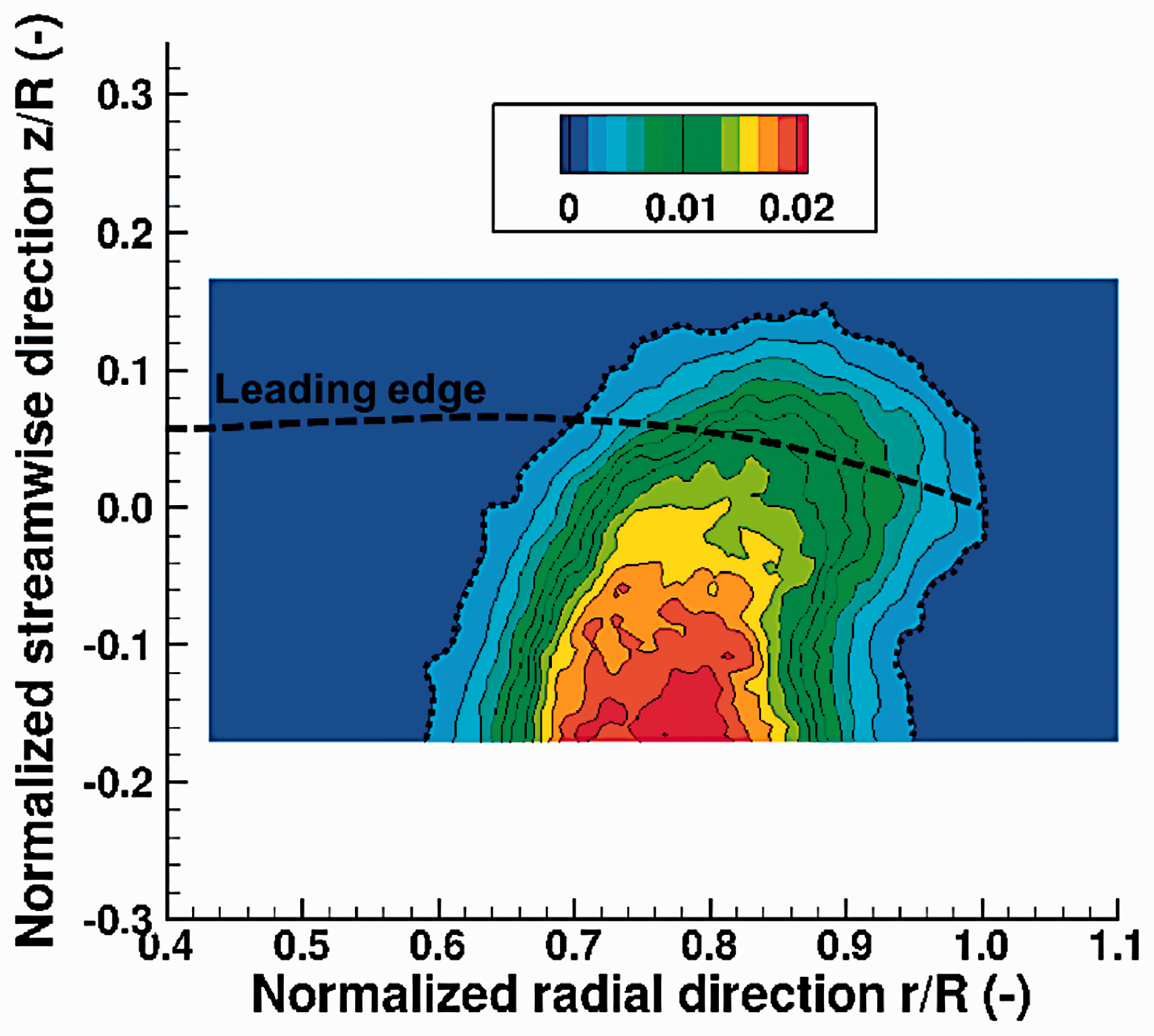
Time-averaged flow field coloured with the normalised streamwise component of the velocity $V_{z} / (ω . R)$ at $z / R = 0.0$ : (a) URANS and (b) LES–LBM. (Data are averaged in the reference frame of the rotor.)

To point out the influence of vortical flows in this configuration, a flow field is extracted at 50% of the chord downstream the trailing edge and coloured with the normalised vorticity magnitude, as shown in Figure 13. The wake generated downstream the blade is then convected by the flow in the streamwise direction, with a higher speed in the vicinity of $r / R \approx 0.7$ . In the case of LES–LBM, a region of intense vorticity is also observed in the tip region, corresponding to the merging of the vorticity generated by the tip vortex and the boundary layer separation. The effect of the tip vortex generated by the previous blade is also visible as a diffuse flow pattern (rather than as a coherent vortex), typical of a vortex breakdown phenomenon. This observation is compatible with the flow dynamics already reported in Figure 2 (however at a much lower Reynolds number). On the contrary, in the case of URANS, only one very intense vorticity region is observed in the tip region, corresponding to a coherent vortex. The trace of the previous vortex, which is still coherent, is also visible below the rotor trailing edge. The conclusion at this step is that the performance discrepancy between LES–LBM and URANS comes from the discrepancy on the behaviour of the tip vortex (breakdown in the case of LES–LBM) and the prediction of a boundary layer separation on the suction side close to the tip in the case of LES–LBM.

Figure 13.

Time-averaged flow field coloured with the vorticity magnitude $ω / Ω$ downstream the trailing edge: (a) URANS and (b) LES–LBM. The dashed line is a projection of the rotor trailing edge. (Data are averaged in the reference frame of the rotor.)

As reported in Lucca-Negro and O’Doherty,³³ an empirical criterion to evaluate the risk of vortex breakdown is to evaluate the Reynolds number based on the vortex characteristics Re_c and the Rossby number Ro, defined as

R o = \frac{V_{c}}{ω_{c} . r_{c}}

(6)

with V_c, ω_c and r_c, the axial velocity, rotation rate and radius of the vortex core, respectively. In the present case,

R e_{c} = 1.5 \times 10^{4}

and Ro = 0.35. The critical value to observe vortex breakdown is to have Ro < 0.65 Spall et al.³⁴ Indeed, based on this consideration, the tip vortex observed in this configuration should breakdown. Several works reported in the literature already pointed out the difficulty to predict the vortex breakdown phenomenon with classical RANS models Morton et al.,³⁵ while methods that are able to simulate, at least partially, the turbulent spectrum, such as LES or DES usually successfully reproduce it.^36,37

Regarding the prediction of acoustic emissions, the question of potential tip vortex breakdown is of major importance: as shown in Figure 13, in the case of vortex breakdown, the turbulence generated by the tip vortex can impact the following blade on a large part of the span, which is not the case if the vortex remains coherent.

The turbulent kinetic energy, normalised with the rotation speed $2. k / {(Ω . R)}^{2}$ , is shown in Figure 14 (from LES–LBM data). Turbulence is mainly observed in the region around $r / R \approx 0.8$ due to the shear layer between the rotor flow and the quiescent flow. Turbulence is also observed above the leading edge, with a turbulent intensity that represents around 5% of the rotor tip speed. This turbulence is produced mainly by the vortex breakdown generated by the previous blade, which then impact the leading edge of the following blade.

Figure 14.

Time-averaged flow field coloured with the normalised turbulent kinetic energy $2. k / {(Ω . R)}^{2}$ upstream the rotor leading edge. (Data are averaged in the reference frame of the rotor.)

The typical turbulent scales seen by the rotor leading edge are estimated by computing the Taylor microscale λ_g. Such turbulent scales are deduced from the two-point correlations in the spanwise direction using the azimutal component of the velocity $V_{θ}$ . Results are shown in Figure 15 for a plane located upstream the rotor leading edge, at 30% of the rotor chord. The typical value for λ_g evolves from $0.02 R$ (internal part of the shear layer) to $0.03 R$ (external part of the shear layer, close to the tip). Indeed, the value of λ_g is roughly constant all over the rotor span, which is an interesting point since it means that a control solution (or an optimised design) will have to deal with only one typical turbulent length scale.

Figure 15.

Normalised Taylor microscale $λ_{g} / R$ , upstream the rotor leading edge. (Data are averaged in the reference frame of the rotor.)

Effect of different designs on acoustic performance

Four designs are investigated with the objective to reduce the blade vortex interaction and thus to increase the acoustic performance. The original geometry is referred as the reference. The second geometry (referred as wavy) is the reference geometry which includes tubercles at the leading edge: the wavelength of the sinusoidal variation is $L / R = 0.28$ , which is equivalent to one blade chord and the amplitude from peak to valley is $A / R = 0.05$ . The use of tubercles at the leading edge is a promising way to increase the aerodynamic³⁸ and acoustic^39,40 performance of profiles. However, it has been poorly investigated for rotating profiles. The third geometry (referred as shifted) is the same as the reference geometry, except that two blades are shifted along the z-axis (streamwise direction): the second blade is shifted by $z / R = - 0.057$ below its initial position and the third blade is shifted by $z / R = + 0.057$ above its initial position.

For the three designs, a breakdown of the tip vortex starts close to the trailing edge. A time-averaged flow field, obtained in the reference frame of the rotor, and coloured with the normalised fluctuations of pressure $p' / (\frac{1}{2} ρ {(Ω . R)}^{2})$ is shown in Figure 16. For the three designs, most of the pressure fluctuations are observed at two locations close to the trailing edge in the vicinity of the rotor tip (tip vortex and suction side separation). The noticeable differences between the three geometries are: (1) for the reference and the wavy leading edge cases, the three blades exhibit the same field of pressure fluctuations, but it is not the case for the shifted blade case (as expected); (2) the source of fluctuations at the rotor tip is reduced with the wavy leading edge; (3) the level of pressure fluctuations in the shifted blade geometry is reduced for two blades (the top-shifted and the middle blade) and is increased for the last one (the bottom-shifted). Compared to the reference geometry, the shifted blade reduces pressure fluctuations at the leading edge, but it has a detrimental impact on the trailing edge noise.

Figure 16.

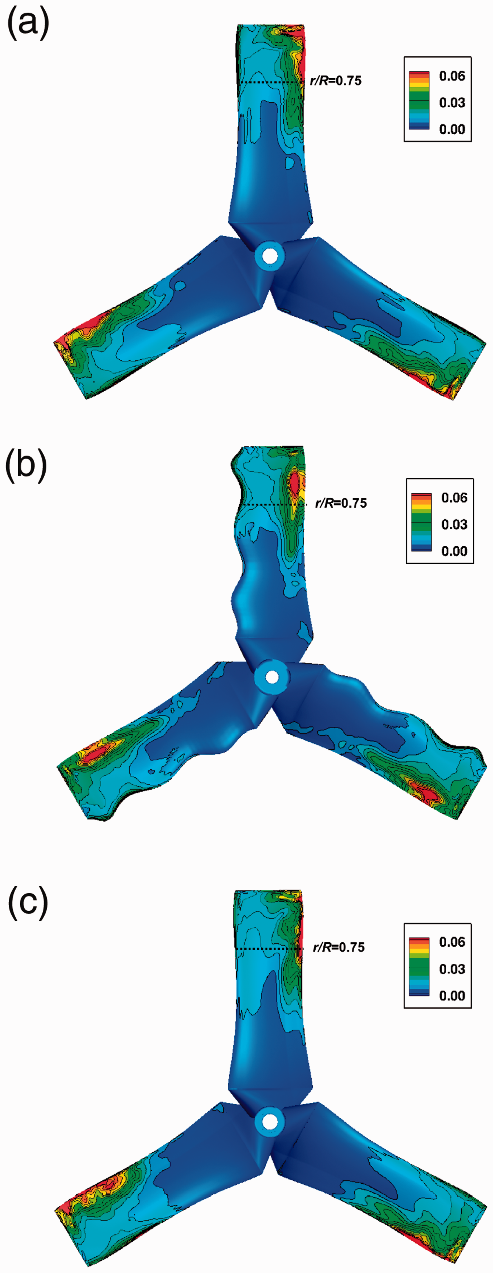
Time-averaged solution on the suction side coloured by the normalised pressure fluctuations $p' / (\frac{1}{2} ρ {(Ω . R)}^{2})$ : (a) reference geometry, (b) wavy leading edge and (c) shifted blades.

The global noise of each configuration can be evaluated at a distance of 10 rotor radii, by integrating the pressure signal on all frequencies, which gives a total noise of (1) 64.9 dB (reference geometry), (2) 64.1 dB (wavy leading edge) and (3) 68.4 dB (shifted blade). The aerodynamic performance is plotted in Figure 17 with respect to the acoustic performance. A validation of these results can be found in Serre et al.^31,41 This analysis of LES–LBM results demonstrates that the adaptation of the leading edge is a potential solution to increase both the aerodynamic and acoustic performance of MAV propeller.

Figure 17.

Comparison of the Figure of Merit (aerodynamic performance) with respect to far-field noise (acoustic performance) for three different designs.

Conclusions

This works shows that LES–LBM has a very good potential to describe the flow related to MAV applications. Three different applications have been investigated, of increasing complexity: a single blade low-Reynolds rotor, a two-bladed rotor in interaction with the ground and a three-bladed rotor optimised for acoustic performance. In all cases, the torque and thrust can be correctly predicted with a good accuracy, but only if a particular care is brought to the near wall grid resolution. The work reported in this paper shows that a correct magnitude order for the grid resolution is to choose $Δ x / C = 0.015$ (with C the chord). Regarding the analysis of flow physics, LES–LBM (as methods based on the resolution of Navier-Stokes equations) has the capability to provide useful information related to turbulence, for example by providing Taylor micro-scale estimations. Such information could help to design more efficient rotor for MAVs. Among the different designs tested to improve the acoustic performance, the use of a wavy leading edge is the most promising approach.

Further investigations include some investigations to assess the potential of LES–LBM to describe near wall flows (use of wall-modelling) and fluid/structure interactions that could be efficiently represented by taken advantage of the immersed boundary approach.

Footnotes

Acknowledgements

Numerical simulations have been performed thanks to the computing center of the Federal University of Toulouse (CALMIP, project p1425) and resources provided by GENCI (project A0042A07178). These supports are greatly acknowledged. Special thanks to the technical team of DAEP at ISAE-Supaero for the acquisition of experimental data and to Orestis Malaspinas and Jonas Latt, from the University of Geneva, for their support on Palabos. The authors also thank CERFACS, for providing the post-processing tool and ONERA for the collaborative work on MAVs.

Declaration of conflicting interests

The author(s) declared no potential conflicts of interest with respect to the research, authorship, and/or publication of this article.

Funding

The author(s) received no financial support for the research, authorship, and/or publication of this article.

References

Piomelli

Reynolds-averaged and wall-modelled large-eddy simulations of impinging jets with embedded azimuthal vortices. Eur J Mech – B/Fluids 2016; 55: 44–66.

Ghias

Mittal

Dong

et al . Large-eddy simulation of the tip flow of a rotor in hover. In: 34th AIAA fluid dynamics conference and exhibit, Portland, OR, USA, 28 June–1 July 2004, paper 2004-2432.

Lallemand

Luo

LS.

Theory of the lattice Boltzmann method: dispersion, dissipation, isotropy, Galilean invariance, and stability. Phys Rev E 2000; 61(6): 6546–62.

D’Humieres

Ginzburg

Krafczy

et al . Multiple relaxation time lattice Boltzmann models in three-dimensions. Phil Trans R Soc A 2002; 360: 437–451.

Latt

Chopard

Lattice Boltzmann method with regularized non-equilibrium distribution functions.

Math Comp Sim 2006; 72: 165–168.

Malaspinas

Chopard

Latt

General regularized boundary condition for multi-speed lattice Boltzmann models. J Comput Fluids 2011; 49: 29–35.

Sagaut

Toward advanced subgrid models for lattice Boltzmann based large-eddy simulation: theoretical formulations.

Comput Math Appl 2010; 59: 2194–2199.

Bodoni

DJ.

Analysis of sponge zones for computational fluid mechanics.

J Comput Phys 2006; 212: 681–702.

Inamuro

Lattice Boltzmann methods for moving boundary. Fluid Dyn Res 2012; 44: 024001.

10.

Malaspinas

Sagaut

Wall model for large eddy simulation based on the lattice Boltzmann method.

J Comput Phys 2014; 275: 25–40.

11.

Shyy

Aono

Chimakurthi

et al . Recent progress in flapping wing aerodynamics and aeroelasticity. Progr Aerosp Sci 2010; 46: 284–327.

12.

Mengaldo

Liska

et al . Immersed boundary lattice Green function methods for external aerodynamics. In: 23rd AIAA computational fluid dynamics conference, 2017: 1–15.

13.

Jardin

David

Root cutout effects on the aerodynamics of a low-aspect-ratio revolving wing.

AIAA J 2017; 55: 2717–2726.

14.

Liska

Colonius

A fast lattice Green’s function method for solving viscous incompressible flows on unbounded domains.

J Comp Phys 2016; 316: 360–384.

15.

Liska

Colonius

A fast immersed boundary method for external incompressible viscous flows using lattice Green’s functions.

J Comp Phys 2017; 331: 257–279.

16.

Lentink

Dickinson

MH.

Rotational accelerations stabilize leading edge vortices on revolving fly wings.

J Exp Biol 2009; 212: 2705–2719.

17.

Jardin

David

Coriolis effects enhance lift on revolving wings.

Phys Rev E 2015; 91: 031001.

18.

Jardin

Coriolis effect and the attachment of the leading edge vortex.

J Fluid Mech 2017; 820: 312–340.

19.

Carr

DeVoria

Ringuette

MJ.

Aspect-ratio effects on rotating wings: circulation and forces.

J Fluid Mech 2015; 767: 497–525.

20.

Medina

Jones

Leading-edge vortex burst on a low-aspect-ratio rotating flat plate.

Phys Rev Fluids 2016; 1: 044501.

21.

Gourdain

Singh

Jardin

et al . Analysis of the turbulent wake generated by a micro-air vehicle hovering near the ground with a Lattice Boltzmann Method. J Am Helicopter Soc 2017; 64: 1–15.

22.

Sanchez-Cuevas

Heredia

Ollero

Characterization of the aerodynamic ground effect and its influence in multirotor control.

Int J Aerosp Eng 2017; 2017: 1823056.

23.

Lakshminarayan

Kalra

Baeder

JD.

Detailed computational investigation of a hovering microscale rotor in ground effect.

AIAA J 2013; 51: 893–909.

24.

Jardin

Prothin

Magana

CG.

Aerodynamic performance of a hovering microrotor in confined environment.

J Am Helicopter Soc 2017; 62: 022008.

25.

Pereira

Chopra

Hover tests of micro aerial vehicle scale shrouded rotors, part i: performance characteristics. J Am Helicopter Soc 2009; 54: 012001.

26.

Rhie

Chow

WL.

Numerical study of the turbulent flow past an airfoil with trailing edge separation.

AIAA J 1983; 21: 1525–1532.

27.

Ferziger

Peric

Computational methods for fluid dynamics. Volume 3rd rev. ed. Berlin: Springer-Verlag, 2002.

28.

Winarto

BEMT algorithm for the prediction of the performance of arbitrary propellers. The Sir Lawrence Wackett Centre for Aerospace Design Technology, Royal Melbourne Institute of Technology, [online resource] available at http://mirror.unpad.ac.id/orari/library/library-non-ict/aero/docs/CoEAL%20report%20BEMT.pdf, 2004.

29.

Farassat

Theory of noise generation from moving bodies with an application to helicopter rotors. NASA Tech. Report, volume R-451, 1975.

30.

Drela

Giles

MB.

Viscous-inviscid analysis of transonic and low Reynolds number airfoils.

AIAA J 1987; 25: 1347–1355.

31.

Serre

Gourdain

Jardin

et al . Analysis of the flow produced by a low-Reynolds rotor optimized for low noise applications. Part ii: acoustics. In: 43rd European rotorcraft forum. Milan, Italy, 12–15 September 2017.

32.

Gourdain

Serre

Jardin

et al . Analysis of the flow produced by a low-Reynolds rotor optimized for low noise applications. Part i: aerodynamics. In: 43rd European rotorcraft forum. Milan, Italy, 12–15 September 2017.

33.

Lucca-Negro

O’Doherty

Vortex breakdown: a review. Progr Energy Combust Sci 2001; 27: 431–481.

34.

Spall

Gatski

Grosh

A criterion for vortex breakdown.

Phys Fluids 1987; 30: 3434.

35.

Morton

Forsythe

Mitchell

et al . DES and RANS simulations of delta wing vortical flows. In: 40th AIAA aerospace sciences meeting and exhibit, Reno, Nevada, 14–17 January 2002, AIAA 2002-0587.

36.

Muller

Kleiser

Large eddy simulation of vortex breakdown in compressible swirling jet flow.

Comput Fluids 2008; 37: 844–856.

37.

Mary

Large eddy simulation of vortex breakdown behind a delta wing.

Heat Fluid Flow 2003; 24: 596–605.

38.

Johari

Henoch

Cosutodio

et al . Effects of leading edge protuberances on airfoil performance. AIAA J 2007; 45: 2634–2642.

39.

Clair

Polacsek

Garrec

et al . Experimental and numerical investigation of turbulence – airfoil reduction using wavy leading edges. AIAA J 2013; 51: 2695–2713.

40.

Chaitanya

Joseph

Narayanan

et al . Performance and mechanism of sinusoidal leading edge serrations for the reduction of turbulence-aerofoil interaction noise. J Fluid Mech 2017; 818: 435–464.

41.

Serre

Gourdain

Jardin

et al . Towards silent micro air vehicles: investigations on an optimized low Reynolds number rotor. J Sound Vibr under review.

Application of a lattice Boltzmann method to some challenges related to micro-air vehicles

Abstract

Keywords

Introduction

Description of the LBM

Single-bladed rotor at low-Reynolds number

Two-bladed rotor in-ground effect

Three-bladed rotor optimised for aero-acoustic performance

URANS

Geometry and grid convergence study

Comparison with measurements

Analysis of the blade vortex interaction

Effect of different designs on acoustic performance

Conclusions

Footnotes

Acknowledgements

Declaration of conflicting interests

Funding

References