
Abstract
The work presented in this paper is part of a project called ARChEaN (Aerodynamic of Rotors in Confined ENvironment) whose objective is to study the interactions of a micro drone rotor with its surroundings in the case of flight in enclosed environments such as those encountered, for example, in archeological exploration of caves. To do so the influence of the environment (walls, ground, ceiling, etc) on the rotor’s aerodynamic performance as well as on the flow field between the rotor and the surroundings is studied. This paper focuses on two different configurations, flight near the ground and flight near a corner (wall and ground), and the results are analyzed and compared to a general free flight case (i.e. far away from any obstacle). In order to carry out this analysis both numerical and experimental approaches are conducted. The objective is to validate the numerical model with the results obtained experimentally and to benefit from the advantages of both approaches in terms of flow analysis. This research work will provide knowledge on how to operate these systems as to minimize the possible negative environment disturbances, reduce power consumption and predict the micro drone’s behaviour during enclosed flights.
Introduction
Since their first developments, drones (unpiloted aircrafts) have revolutionized flight, opening a wide range of new possibilities that were unconceivable some decades ago. Drones allow us to go further than ever and their applications, which go from military uses to observation, exploration, meteorology, audio-visuals etc., are nowadays growing exponentially in parallel to new technological developments. Their versatility and flexibility offer significant opportunities for new research and development projects.
The present study focuses on how a micro rotor of a drone at stationary flight (i.e. hovering flight) interacts with its environment. The aerodynamic forces experienced by the micro rotor and the velocity of the surrounding fluid are evaluated and correlated. The analysis and comprehension of this correlation will allow to define models that represent the physics involved in these situations and to integrate them in the drone’s control laws. The outcomes should therefore help improve the efficiency of drones flying in confined spaces and help reduce the effects of detrimental phenomena on the local environment (e.g. brownout phenomenon during archaeological exploration).
In particular, the scope of this paper is to carry out new configuration cases and to study them using both numerical and experimental approaches, in parallel, in order to compare them with one another and to benefit from the advantages that each one has to offer in terms of flow and performance analysis.
In what follows, the configuration of the study is detailed, the numerical and experimental approaches are presented in order to explain and analyze the results obtained with each one of them and finally, both approaches are compared. A list of nomenclature and a list of figures as well as literature references are included at the end of the manuscript in order to aid the reader in his/her understanding of the text.
The scientific literature is scarce regarding investigations of the aerodynamics of micro drone flight in closed environments. While out-of-ground effect (OGE) and in-ground effect (IGE) have been addressed by previous works,1–5 the vast majority of available literature considers helicopter flight for which the Reynolds number is large. Hence, results do not necessarily apply to present cases where Reynolds numbers are relatively small, typically on the order of 104–105. On the other hand, there are, to the author’s knowledge, no studies that report flight in corner effect, which is a relatively common situation in real-life applications.
Geometry and configurations
Rotor geometry
As previously mentioned, two approaches are carried out in the present project. First, an experimental approach is conducted as a reference. Second, numerical simulations are conducted to achieve a more thorough knowledge of the aerodynamics involved. The two approaches are compared and validated with one another.
The geometry of the rotor selected for every test cases carried out in this project is a two-bladed rotor with rectangular blades of 100-mm span and 25-mm chord length (c), having an aspect ratio (AR) of 4. As shown in Figure 1, the radius of the rotor (R) is 125 mm. That is, there is a 25-mm root cut-out. The very same rotor geometry is used for numerical simulations. The blades have a constant pitch angle of 15°. The geometry is chosen simply to facilitate analysis, especially regarding force distribution along the blade, which are hence not influenced by blade twist and chord variations. It is also similar to that used in previous work by the authors. 6

Top and side views of the rotor geometry.
Confined configurations
A closed environment can be parameterized using many variables depending on the types of obstacles encountered, the obstacle-to-obstacle distances and drone-to-obstacle distances, etc. In order to simplify the problem and be able to study the phenomena in a general manner, different test cases have been chosen to model representative enclosed configurations. These configurations are briefly listed below. Illustration is also provided in Figure 2.

Configurations of rotor interacting with walls.
Out-of-ground effect (OGE): the reference, free case without obstacles.
In ground effect (IGE): presence of a wall downstream of the rotor.
In ceiling effect (ICE): presence of a wall upstream of the rotor.
In wall effect (IWE): presence of a wall perpendicular to the rotor plane.
In channel effect (IChE): presence of two walls, one upstream and one downstream of the rotor.
In low corner effect (ILoCE): presence of two walls, one downstream of the rotor and the other perpendicular to the rotor plane.
In upper corner effect (IUpCE): presence of two walls, one upstream of the rotor and the other perpendicular to the rotor plane.
OGE, IGE, ICE, IChE cases are reported in Jardin et al.,6 and we presently focus on the ILoCE configuration, which we compare with OGE and IGE cases.
The ILoCE refers to the situation where an aircraft flies or hovers close to the ground (flat surface in this case) and close to a perpendicular wall (flat surface in this case) simultaneously. In what follows, all experiments and simulations are conducted in hovering flight conditions.
Within this configuration, three different cases are analyzed each with a different rotor-to-ground and rotor-to-wall distance. To characterize each case, the dimensionless rotor-to-ground distance h/R is used and we introduce a new dimensionless distance, d/R where d is the distance from the centre of the rotor to the wall and R is the rotor radius.
The cases studied within this configuration will therefore be referred to as
ILoCE h/R = 2 d/R = 2 ILoCE h/R = 2 d/R = 3 ILoCE h/R = 3 d/R = 2
Similarly to the IGE configuration reported in Jardin et al., 6 the objective is to fly at a constant thrust value of 2 N. This value is somehow arbitrary, yet it is set as being representative of the thrust needed for an MAV with dimensions on the order of 20 cm to hover. Experimental tests on each of the above-mentioned configurations are carried out to obtain the rotation speeds that satisfy this thrust constraint, which will then be imposed in the numerical simulations and used to obtain the blade force distribution and the behaviour of the fluid around the rotor. Note that typical rotation speeds are on the order of 3500 r/min, which yields a typical tip Reynolds number on the order of 78,000. In this regime, it is believed that viscous effects have significant effects which preclude application of inviscid theory for numerical analysis. Additionally, in the ILoCE case, further experimental analysis of the wake is carried out using particle image velocimetry (PIV) measurements. Further information on both numerical and experimental approaches is detailed in the corresponding sections below.
Experimental approach
Force measurements
As previously mentioned, all configurations in this paper are carried out considering a 2 N constant thrust value. The rotation speed corresponding to this thrust value may change significantly depending on the configuration studied. These speeds have therefore been obtained experimentally. The apparatus used to obtain the experimental values plays a crucial role in the results obtained. Therefore, the main components are detailed below, as well as their importance in the experiment.
The rotor frame of reference is shown in Figure 3 to help understand the set-up. The balance has a different frame of reference as will be explained further on but the measurements are converted to the rotor frame of reference since the results will be expressed as seen by the rotor.

Rotor frame of reference.
The balance used to measure forces and moments in three directions is shown in Figure 4. It is 21.6 mm long and has a diameter of 25 mm. The sensing range of the balance is 125 N for the forces along the X and Y axis, 500 N along the Z axis and 3 Nm for each moment. The maximum error in a measurement given by the manufacturer, and verified in our laboratory, is of 1% for forces and 1.25% for moments.

Six-component force/torque balance (ATI Nano 25).
A 350 W brushless MikroKopter® MK3638 motor is connected to the rotor providing it with the necessary power for rotation. The presence of the ground is modelled using nine assembled 30 by 30 cm2 PMMA plates, leading to an overall surface of 90 by 90 cm2. Similarly, a wall made out of a single piece is placed perpendicularly to it to model the wall.
A displacement system is used to place the rotor at different distances from the ground and the wall. A steel support rod is used to connect the displacement system and the motor ensemble. The data of each measurement point is acquired at constant rotational speed and static conditions reproducing rotor hovering. Four different measurements are performed for each set of velocity-position to verify the measurement’s repeatability. During the tests, the blade’s azimuthal position is acquired and the atmospheric conditions (Tatm, Patm) measured for data normalization. The azimuth position measurement is performed by an optical encoder having a resolution of 500 dots per revolution. This allows us to have a very high accuracy in position (0.72°) and speed (0.12 r/min).
The convergence of signal-spectrums for all variables is checked. When convergence is achieved, the mean of each variable is calculated using 50,000 samples.
PIV measurements
A PIV analysis is carried out to characterize the behaviour of the fluid surrounding the rotor in ILoCE cases.
For each ILoCE case the rotor plane of symmetry, which is perpendicular to the ground and to the wall, will be analyzed as well as other planes parallel to it to obtain a three-dimensional (3D) velocity distribution of the fluid volume centered around the rotor, Figure 5.

Locations of PIV planes and PIV setup. PIV: particle image velocimetry.
Tracer particles chosen for this experiment are olive oil particles (mean diameter of 1 micron) produced by a TOPAS ATM 210 H generator. The mixing of the particles is carried out in the whole closed room where the experiments take place, prior to the acquisition phase.
The laser used in these experiments is a DualPower Bernouilli PIV 200-15. It is a pulse laser with double cavity which emits light with 532 nm wavelength at a frequency up to 15 Hz. It delivers an energy pulse of 2 × 200 mJ, which is spread onto a laser sheet by means of a cylindrical lens. For the acquisition of two consecutive double-frame images each cavity emits a pulse with a time step (which corresponds to the time between two images) that ensures a maximum particle image displacement of 7 to 8 pixels. The thickness of the laser sheet is set to 1.5 mm.
For each measurement plane, 1000 pairs of stereoscopic PIV images are captured with two high-resolution cameras. Each image of 16 MP resolution is captured at a frequency of 2 Hz, with a time step of 80 μs between two consecutive images. The cameras have a Scheimpflug setup which enables them to work in conditions such that the object, the objective plane and the image plane have a common axis. In this way, the whole plane can be captured without the need for large lens aperture.
“DynamicStudio v4” software developed by Dantec Dynamics is used to cross-correlate these consecutive pairs of double-framed images, hence enabling the computation of corresponding velocity vectors of tracer particles and determining the actual flow field behaviour. An overall view of the setup is shown in Figure 5.
Numerical approach
The numerical simulations are carried out using the commercial flow solver STARCCM+. The latter solves the unsteady Reynolds Averaged Navier-Stokes equations (URANS), under their incompressible form, using a cell-centred finite volume approach. Momentum and continuity equations are solved in an uncoupled way using a predictor-corrector approach (SIMPLE-type algorithm). Second order schemes are used for both spatial and temporal discretizations. Turbulence closure is achieved using a Spalart-Allmaras model.
Boundary conditions
Different combinations of the following boundary conditions are imposed depending on the configuration being simulated, see Table 1:
Boundary conditions used for different test cases

OGE: out-of-ground effect; IGE: In ground effect, ILoCE: In low corner effect.
Stagnation inlet: defines the total pressure at the inlet.
Pressure outlet: defines the static pressure at the outlet.
Wall: represents an impermeable surface that separates the fluid and the solid medium. A non-slip condition is imposed.
Meshes
The two-bladed rotor presented in previous sections is implemented in the STARCCM+ flow solver. The two blades are designed using Gambit-ANSYS software. Only the two blades of the rotor are generated, i.e. without the hub, in order to actually analyze the aerodynamics of the blades without the influence of any other elements.
Two first 3D-O-Grid meshes enclosing the blades (one for each blade) are generated using Gambit-ANSYS, Figure 6. Cells at the blade surface have face sizes of 1–2 mm2 in the first layers of the boundary layer mesh, Figure 7. Each of these meshes constitute an individual fluid region that is rotated together with the blades. These regions contain approximately 920,000 cells, with dimensions 125 mm in length and 25 by 50 mm in the chord plane.

Blade’s region mesh for numerical simulations.

Blade surface mesh
A third background, trimmer mesh of the fluid volume, is generated using StarCCM+. The latter is steady (as opposed to the first two meshes that rotate with the blades) and consists of approximately 18 million trimmed cells. To ensure reduced numerical dissipation due to interpolation between rotating and background meshes, the cell size of the background mesh in the vicinity of the rotating mesh is set to be similar to that of the outer boundary of the rotating mesh, i.e. on the order of 1 mm. This size then increases progressively to 5 mm within the domain.
At each time step, continuous interpolation between the trimmer mesh of the external, background region and the O-grid rotating mesh of the blade’s region allows fluid exchange between both regions. Note that this procedure is generally referred to as “Chimera Grid Method” or “Overlap Method”.
For the OGE case, the rotor is placed at a distance of 12.5 radius below the horizontal upper boundary condition, which corresponds to the stagnation inlet condition, and at a distance of 12.5 radius of the lower boundary condition, which corresponds to the pressure outlet condition. In the IGE configurations, the lower and upper walls are positioned at the different desired simulation distances.
To ensure convergence of the results with respect to spatial and temporal resolutions, simulations are carried out with a finer and a coarser mesh size as well as with a shorter and a longer time step. Every rotor rotation is divided into 180 time steps and each time step has 20 inner iterations. Each simulation is carried out until 100 rotor rotations are reached in the ILoCE cases and 50 rotor rotations in the IGE cases. For each case, convergence of the simulations with respect to initial transients is checked by looking at the values of the blade forces reached throughout the simulation, Figure 8.

Example of convergence in a simulation of an IGE case. IGE: In ground effect.
Results
Thrust values
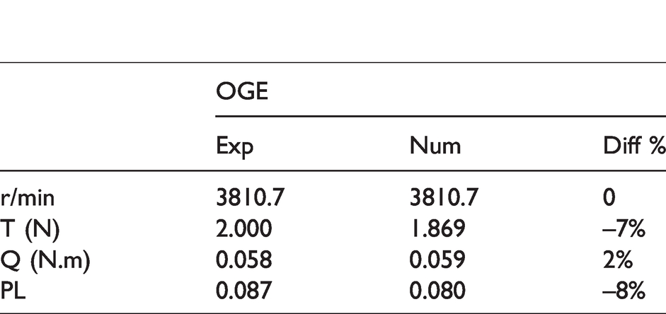
As previously explained, to ensure that the results correspond to a constant thrust value of 2 N, the rotation speed for each case is found experimentally. Then the rotation speed value is imposed in the numerical simulations and the results obtained are compared to those obtained experimentally. These results are shown below, demonstrating consistency between both approaches, Tables 2 and 3.
Numerical and experimental comparison for out-of-ground effect (OGE) cases.
Numerical and experimental comparison for IGE cases.

IGE: In ground effect.
It can be observed that the numerical approach tends to underestimate the thrust value and slightly overestimate torque. Because of technical issues it was not possible to repeat the same procedure for all ILoCE cases. That is, the rotation speed leading to a 2 N thrust for h/R = 2 d/R = 2 was used for all ILoCE cases and it was verified that the resulting thrust remains close to 2 N. The corresponding value for r/min is 4041.
Force distribution on the blades
IGE case
In this section, the lift and drag distributions along the blade are investigated through numerical simulations in order to understand its behaviour in relation to the rotor’s distance from the ground and/or wall. Again, recall that to obtain a constant thrust value of approximately 2 N, the values from experimental measurements are used to find the rotation speed required to achieve the desired thrust. This speed is then used in StarCCM+. Thus, the area under each mean lift distribution curve is always approximately 2 N if both blades are considered. Figure 9 is obtained by calculating the mean force distributions over the last rotation, after 50 rotor rotations have been reached to ensure convergence with respect to initial transients. The reference case is the OGE case and as expected, the closer the rotor is placed to the ground the more observable its influence is on the blade force distribution. Similarly, the IGE h/R = 2 force distribution is extremely close to that of the OGE case.

Mean of lift/drag distribution for different IGE Cases (Numerical simulations). IGE: In ground effect.

ILoCE Diagram. ILoCE: In low corner effect.
Also, while the lift beyond ¾ blade span for the h/R = 1 case shows small variations with respect to that obtained for the h/R = 2 case, variations near the hub are largely noticeable. Conversely, the h/R = 0.25 and h/R = 0.5 cases are far from other curves all along the blade and rather similar to one another. Additionally, it is important to observe how the closer the rotor is to the ground the smaller the mean lift beyond ¾ blade span. The opposite is true as we approach the centre of the rotor. Therefore, it can be stated that the closer the rotor is to the ground the more uniform the mean lift distribution becomes. The same observations are true for the mean drag distributions.
ILoCE case
Figure 10 provides some clarification to better understand the results that will be presented in this section. Firstly, a rotation starts with the rotor perpendicular to the wall, with blade 1 being the blade that is the closest to the wall in this position. Secondly, the rotation is anticlockwise and the angle of rotation is measured as shown in the diagram.
In the ILoCE case, Figure 11 shows that the total lift and drag values of blade 1 decrease as the blade moves away from its initial position perpendicular to the wall until it reaches a position parallel to the wall where the forces increase again. This means of course, that simultaneously, the forces on blade 2 increase because a total 2 N global thrust is achieved. It can be observed that the effect is most noticeable around ¾ span since the forces at the tip and near the hub remain roughly constant. The corner effect can also be represented as shown in Figure 12, which shows the force distribution as seen from above for different local rotor radius. The non-symmetrical effect caused by the presence of the wall can be observed only for the larger local radii. Similarly, this effect can be observed in the force colour maps in Figure 13, where it is shown that the asymmetry on each blade is opposite from one another.

Mean of lift/drag distribution for different ILoCE Cases (Numerical). ILoCE: In low corner effect.

Lift distribution ILoCE h/R = 2 d/R = 2 (Numerical). ILoCE: In low corner effect.

Lift (left column) and Drag (Right column) force representation for the blade 1 (upper Line) and blade 2 (lower line) (Numerical).
Wake
Although the analysis of the fluid flow does not lead to a direct quantification of the effects seen by the rotor, it helps understand the physical phenomena that occur in the vicinity of the rotor by allowing direct visualization of the fluid-structure interaction and hence provides insight into how modifications of the flow field affect aerodynamic performance. In this section, diagrams of iso-velocity in a plane section are shown with the out-of-plane velocity component represented using colour contours as to obtain a 3D representation of the flow. The topologies of the flow are discussed and compared on the basis of numerical simulations and PIV measurements are added for the ILoCE case.
OGE case
For the reference OGE case, Figure 14 shows a perfectly symmetrical flow, as expected. The out-of-plane velocity shows the anticlockwise rotation of the rotor with fluid coming in the plane on the right-hand side and out of the plane on the left-hand side.
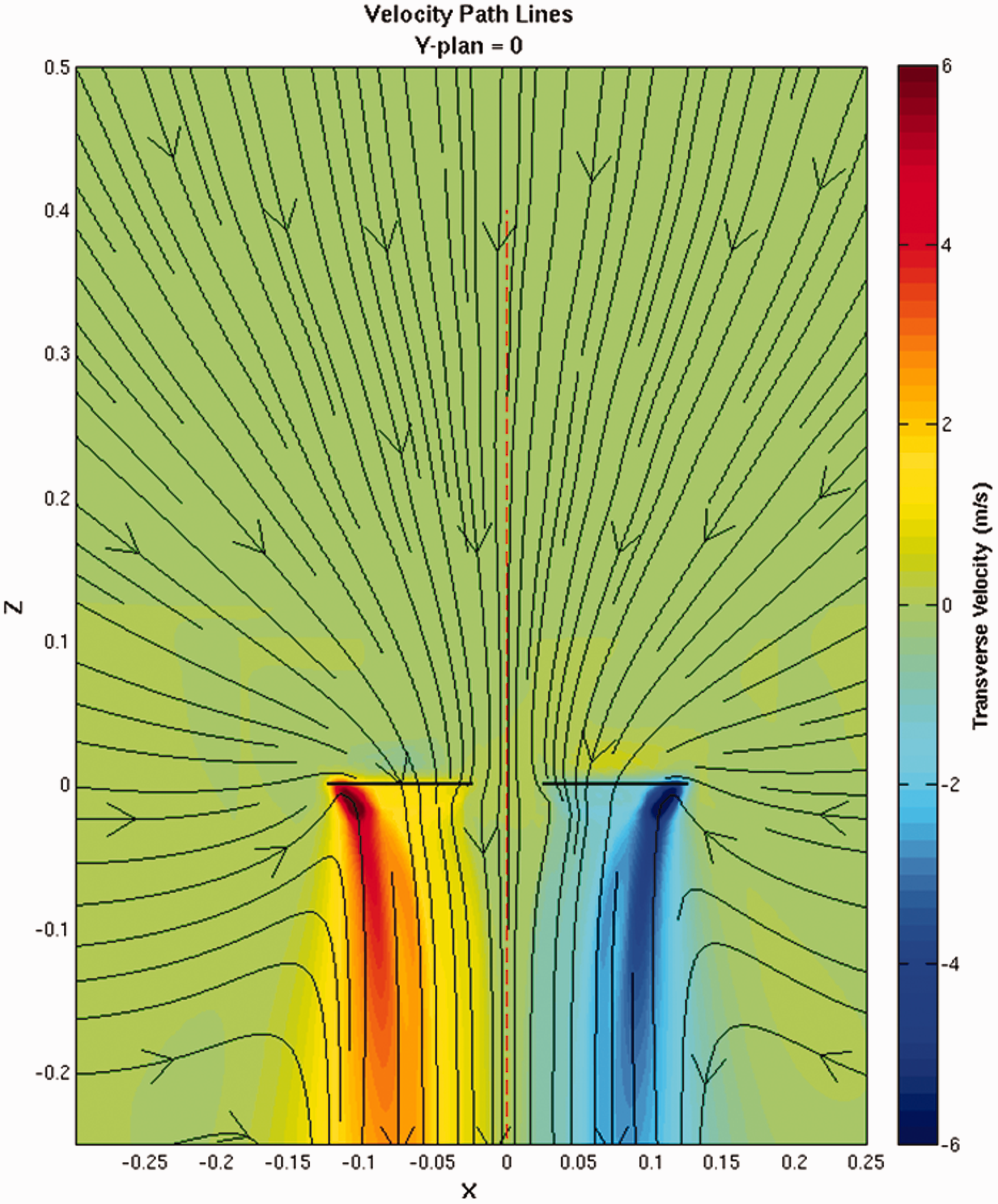
Mean velocity fields OGE (Numerical simulations). OGE: out-of-ground effect.
IGE case
The four IGE cases show how the rotor wake is deformed by the presence of the ground, see for example case h/R = 2 in Figure 15. The effect is less visible as the rotor moves away from the ground and the IGE h/R = 2 case shows that the effect of the ground is almost absent. However, the other cases show how the rotor wake jet is expanded due to the presence of the ground and how the flow recirculates upward and impinges the rotor from underneath. It is important to remember that the hub has not been simulated which means that some figures show the flow passing upwards in between the blades, which would not occur in a real rotor with a blade hub.

Mean velocity fields IGE – h/R = 2 (Numerical simulations). IGE: In ground effect.
ILCoE case
In Figure 16, left, we can observe the topology of the rotor wake in corner effect. A toroid can be observed in the blade hub area where the fluid goes into the plane on the right-hand side of the hub and out of the plane on the left-hand side. It is clear that the flow is not symmetrical in this case. Two vortices can be observed underneath the rotor and a source point is formed due to the presence of the wall. The interaction with the wall also causes this vortex to rise above the rotor and to interact with it from above. Similarly, Figure 16, right, shows the same figure with results obtained from PIV. It can be observed that the PIV captures the same source pattern near the wall and how the vortex rises above the rotor. However, the vortices near the ground do not appear. This might be due to the number of PIV snapshots (i.e. 1000 acquisitions), which ensures statistical convergence of velocity derivatives in most regions but may not ensure perfect convergence in regions where laser reflections occur (i.e. typically near the wall and ground).

Mean velocity fields ILoCE – h/R = 2 – d/R = 2 (Numerical simulations: Left/Experiments: Right). ILoCE: In low corner effect.
Figure 17 displays flow fields obtained in planes adjacent to the midplane y = 0. The source point, singularity observed in Figure 16 appears to be a cut in a 3D vortex whose core moves upward with increasing distance from the y = 0 plane. That is, horn-shaped vortices appear on both sides of the y = 0 plane and connect at the singularity observed as a source point, Figure 16. Comparison between negative and positive y planes demonstrates rather similar flow patterns, with in-plane streamlines exhibiting symmetry with respect to the y = 0 plane. In other words, the direction of rotation of the rotor (which renders the configuration non-symmetrical) has a relatively weak influence on the flow pattern.
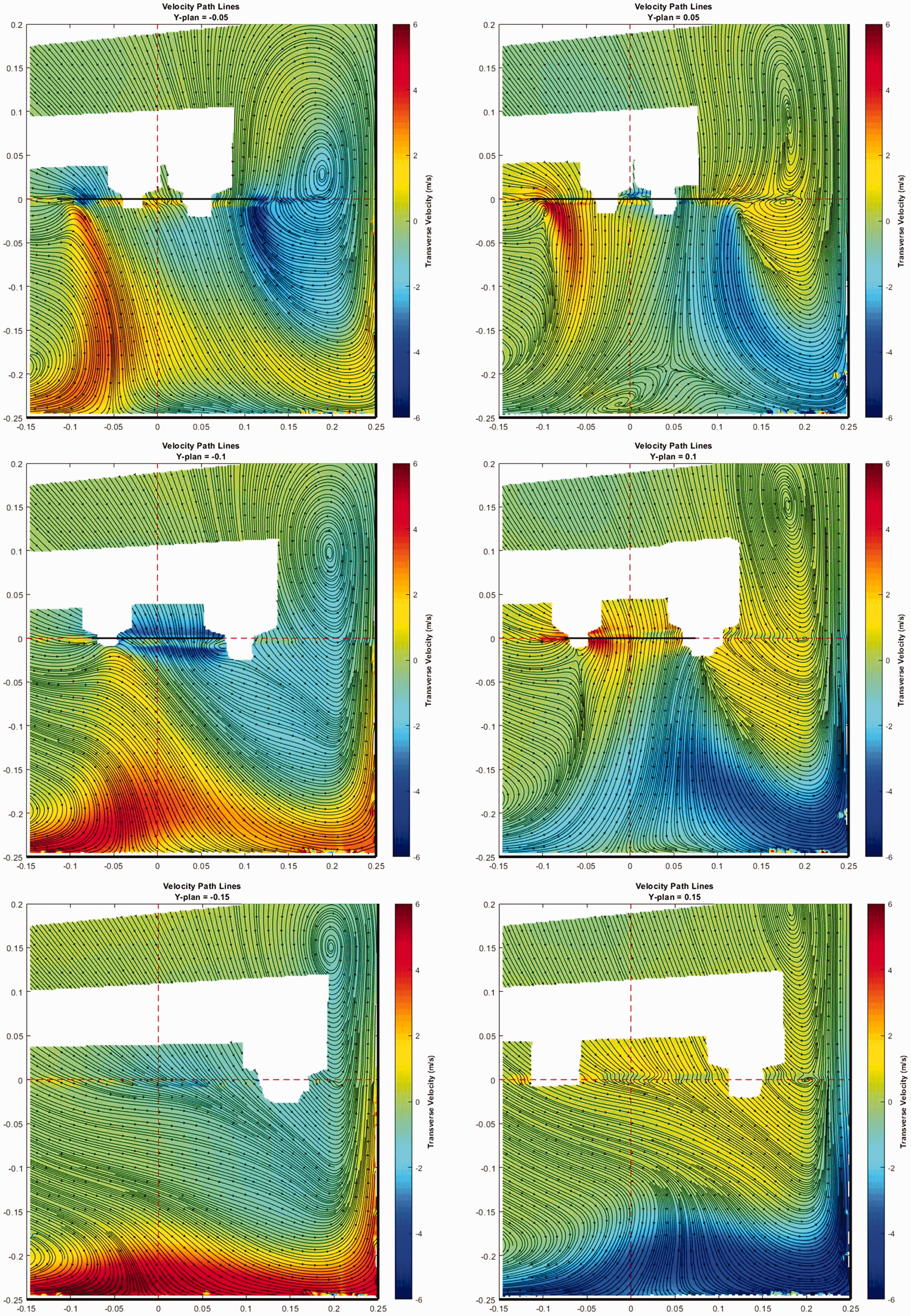
Experimental mean velocity fields for 6 Y-positions ILoCE – h/R = 2 – d/R = 2. ILoCE: In low corner effect.
Conclusion and future work
Due to their small dimensions and versatility, drones can be designed to perform missions in confined environments. Many fields of applications, such as archeology and nuclear security, could greatly benefit from these developments. A way to enhance flight robustness is to understand how the rotor of a hovering drone responds to wall proximity in terms of its effect on the flow field, the force distribution it experiences and its aerodynamic performance. These three effects were studied in this work and the physical link between them was analyzed to improve the physical understanding of confined flight.
While the present study revealed interesting features characterizing a rotor in ground and in corner effect, further analysis is required, which requires additional PIV measurements and numerical simulations. This is the scope of ongoing work.
Additionally, other configurations mentioned in the geometry and configurations section, such as the upper corner effect and 3D corner effect will also be investigated to provide a more complete picture and eventually enable drone flight in real confined environments. These investigations will again rely on both numerical and experimental approaches. In this context, multiple rotors, rather than isolated rotors, could be addressed. In particular, because one rotor influences the whole surrounding flow which in turn may influence other rotors performance, it is likely that multiple rotor configurations do not simply derive from linear superposition of isolated rotor configurations. Moreover, differences between rotors will result in significant rolling and pitching torques that are presumably detrimental to controllability of the aircraft.
Another future investigation is to consider dynamic flight rather than static flight, as was done in this paper. The resulting flow field may be greatly affected for sufficiently large speeds that make quasi-steady approaches unsuitable. This can be achieved experimentally by replacing the displacement rod described in the experimental setup section by a robotic arm which would move the drone following prescribed motions.
Footnotes
Declaration of conflicting interests
The author(s) declared no potential conflicts of interest with respect to the research, authorship, and/or publication of this article.
Funding
The author(s) received no financial support for the research, authorship, and/or publication of this article.