Sage Journals: Discover world-class research

Abstract

Wheel configuration is the great significance for vehicle aerodynamics, and understanding the influences of wheel configuration on the aerodynamic behaviors of vehicle is a good choice to effectively decrease aerodynamic drag and optimize aerodynamic efficiency. In this study, the aerodynamic characteristics of Ahmed body mounted with different wheels configurations were evaluated by Computational Fluid Dynamics (CFD) using the lattice Boltzmann method. The simulation results were compared with published research data to study resolutions independence and verify the accuracy of the numerical method. The four opening areas of the rim were used to form different wheel configurations. The result showed that the drag of the front and rear wheels increases linearly with the increase of the rim opening area, while the drag of the bodywork decreases linearly. Downstream the body region, the structures of vortex shedding and surface pressure presented differences for each wheel configuration, which further resulted in different fluctuation intensities in wake vortices. The order of the width of the wake vortices in wheel region was as follows: W₄> W3 > W2 > W1. The front wheel had a mainly affect on the time-averaged slipstream peak around the outside of vehicle body.

Keywords

Wheel configuration aerodynamic behavior flow characteristic numerical investigation lattice Boltzmann method

Introduction

High speed development of social economy and auto industry promotes the rapid incensement of passenger car sales in the world, and the passenger car is a vital travel tool in modern society. However, it’s reported that 45% of the total energy use and emission in transportation comes from passenger cars.¹ Therefore, new regulations, for example, WLTP, on fuel consumption and vehicle emissions are becoming stricter than previous ones. It is reported that reducing aerodynamic drag by 10% can decrease fuel consumption by about 2%–3%.² Due to the diversity in real vehicle geometries, and to better understand the aerodynamic drag generation mechanisms and flow field characteristics, lots of car physical models are established and used to widely conduct the study of flow separation and vortex shedding. Among the lots of the car physical models, the so-called Ahmed body is one of the most prevalently simplified models for the aerodynamics performance of road vehicles, and lots of research results, for example, flow separation, wake structure and aerodynamic drag reduction methods, has been derived from the Ahmed body.^3–6

Thus, the drag reduction is mainly realized by optimizing car styling to reduce carbon emission and enhance erergy effciency, which has been one of the hottest research points in the industrial and academic, but it will encounter more difficulties in further tapping the potential.⁷ At present, many investigations, both wind tunnel test and numerical simulation, have been confirmed that the drag contributions from wheels takes in 25% of the automotive drag. When vehicle shape optimization become a bottleneck problem, the wheel drag reduction maybe a critical component of optimization of vehicle aerodynamic performance.^8,9 The flow field around the wheel is complex, and the rotation effect of the wheel will result in flow separation and there are some obvious vortex structures. The wheel configurations not only affect the vehicle aerodynamic drag, but also influence the brake cooling system. After the wheel optimization design, the aerodynamic drag of the car is reduced by 3.17% and average surface convective heat transfer coefficient of brake discs is increased by 9.31%.¹⁰ Besides, the complicated geometry and parameters of the wheel have an impact on the flow characteristics around the rotation wheels. To reveal the aerodynamic mechanism of wheel, a large amount of research on wheel geometry and parameters has been carried out using physical test and model simulation. The effect of the coverage area on drag coefficient is greatest and increasing the coverage area typically reduced the flow through the rim and the drag caused by the jetting vortex.¹¹ The increase in spoke curvature will increase the vehicle drag coefficient, while smaller spoke offset distance is beneficial to the drag reduction.¹² The difference of spokes affects the flow separation and field characteristics of the wheel region, resulting in the change of the vortex system and the aerodynamic resistance of the wheel.^13,14 It is pointed out that the smooth transition of spokes can reduce the jet vortex intensity in the wheel area and reduce the wheel aerodynamic drag.¹⁵ The wheel with fully covered using a flat surface can restrain flow separation and the drag of the vehicle could be decreased by more than 5%.¹⁶ To obtain the drag reduction effect as much as possible, lots of electric vehicles prefer the wheels with larger coverage area to reduce aerodynamic drag and extend travel range, as shown in Figure 1. The above literature mainly takes the isolated wheel as the research object, and analyzes the influence of different geometric parameters on the wheel and vehicle aerodynamic drag. How do the wheel configurations, especially the coverage area, impact the flow field and the aerodynamic behavior of the wheel and vehicle has not yet been deeply performed, which should be further systematic study.

Figure 1.

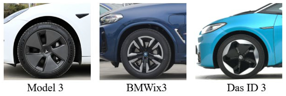
Different wheel shapes of the EV.

The wind tunnel test is a powerful tool for researching aerodynamics,^17–19 however, lots of important flow information, for example, the jetting vortices, is hard to be captured in wind tunnel experiment.²⁰ Recently, Computational fluid dynamics (CFD) method has been occupied the dominant role in studying the flow fields of the wheel. Improving the accuracy of aerodynamic simulation needs to accurately simulate wheel rotation, which is important to accurately predict wheel aerodynamic drag and flow field characteristics, it is because the differences between flow field of the rotation and static wheel are significant.^21,22 There are three common methods used to simulate the wheel rotation in previous studies^23–25: Moving Reference Frame (MRF), Rotating Wall (RW), and Sliding Mesh (SM). The MRF method is applied to the fluid region defined by the user in a local coordinate system, and the rotation effect will be introduced into all regional elements.²⁶ The RW method is one of the most commonly approaches used to model rotating parts, however, many surfaces cannot be modeled correctly with the method due to the geometric complexity of wheels and tires.²⁷ The SM method is realized as a rigid body motion and it can be easily applied to the rims, and the running time is significantly increased because the grid rotates physically at each time step. Besides, the SM has the highest precision in these methods.²⁸

The three common simulation methods mentioned above has not enough capability to simulate the true rotation of the tread tire. In order to correctly represent the tire geometry and boundary conditions for modeling wheel rotation, a composite rotation method was used to study wheel aerodynamic characteristics, in which the rims were set as SM and the tire was set as RM, the simulation results show that the error of the composite rotation method is 1.23% compared with the experimental value, and the calculation efficiency is increased by 15% relative to the SM method²⁹; the hybrid MRFg (Moving Reference Frame-grooves) approach was used to simulate the rotational behavior of tire and wheel and the MRFg is a promising method to solve the rotation problem of a wheels with complex tread pattern.³⁰ A non-ignorable problem for the hybrid approach is that the different split types may affect the accuracy of simulation results. Besides, the model simplification, cell size, and parameters setting have greater influence on the prediction accuracy and computational efficiency for wheel aerodynamics. An approach is applied to model wheel rotation in this study, which has been used to rotate parts such as in the case of bionic flapping wing aircraft and impeller tidal turbine.^31,32

Large eddy simulation (LES) can resolve the unsteady large-scale turbulent motions accurately, however, the method is often not computationally feasible, as it suffers from a very restrictive grid resolution requirement near the wall.³³ The lattice Boltzmann method (LBM) considers the advection and collision of fluid particles at the mesoscopic level, which shows promise to address some of as detached unsteady flows.³⁴ In this work, the LES method based on LBM solver was utilized to investigate the aerodynamic characteristics of the Ahmed body mounted with different wheel configurations. The structure of this paper was organized as follows. We introduced the numerical details and then compared with the available experimental data to verify accuracy of the method. Besides, we systematically analyzed aerodynamic characteristics around the model, including the aerodynamic drag, flow fields, slipstream, and vorticity profiles. Finally, the conclusions were given.

Numerical details

Geometry model

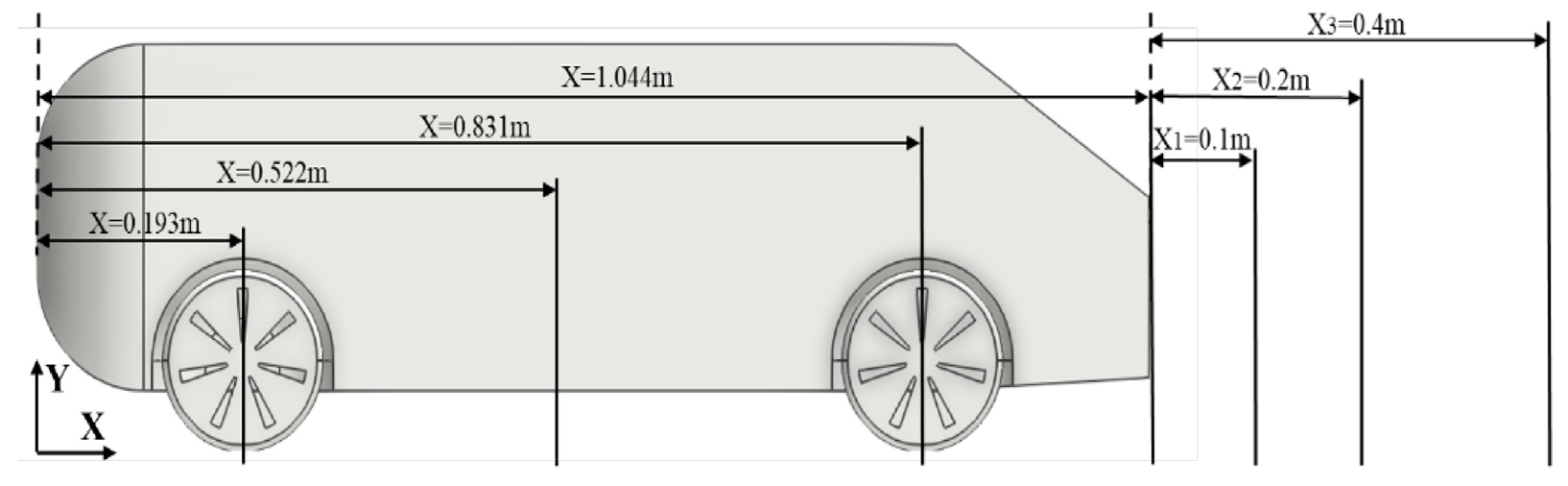
In 1984, in order to systematically study the wake structure of automobiles, Ahmed et al. proposed the Ahmed et al. body, which is the simplified car body model by reasonably abstracting and simplifying the real car.³⁵ The basic sizes are presented in Figure 2, the length of the model is 1044 (value in mm), defined as the characteristic length H, and its size is equivalent to a quarter of the real car one. The Ahmed body belongs to the car body scale model, which is composed of the blunt front end, the middle car body, the slant plane, the tail vertical plane and the four cylinders supporting the model. The front end is inverted round to reduce the flow separation; the middle car body is a rectangular box ensure that air flow through the front end fully develops into a turbulent boundary layer before reaching the tail, so that the near flow structure and aerodynamic performance depend largely on the tail backflow area and the slant angle α. The Ahmed model was studied for various specific slant angle α, between 0° and 40°, and a nonlinear relation existed between the slant angle α values and aerodynamic drag coefficients. For current work, the slant angle 35° was selected because it corresponded to a stable aerodynamic configuration and low drag coefficient of 0.275.

Figure 2.

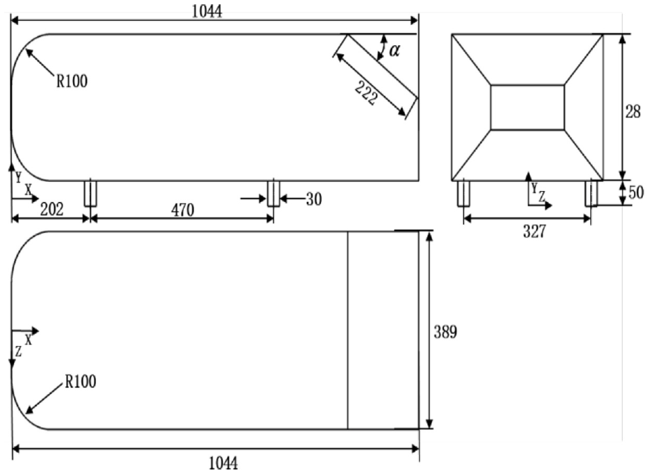
Sizes of Ahmed body in unit mm.

Computational domain and boundary conditions

Figure 3 shows the size of computation domain, and the length, width and height of computational domain were 9, 3, and 2H, respectively. The front end of the model was projected in the plane area S = 0.112 m² perpendicular to the longitudinal axis, The blockage ratio was 1.79%, which met the calculation requirements. To weaken the boundary layer effects and ensure the fully development of the wake, the Ahmed model was placed 2.5H from the inlet boundary and 6.5H from the outlet boundary. A uniform velocity profile was assigned with the inlet boundary, and the outlet was set as the pressure outlet with the reference pressure of 0 Pa, and the periodic boundary condition was set as the two side faces; the ground and top of the domain were set as a free-slip wall with no velocity. All the Ahmed model surfaces were treated as no-slip wall boundary conditions.

Figure 3.

The flow domain for simulations: (a) front view and (b) side view.

Numerical methods

Different from the traditional method of the finite difference method or finite volume method, the XFlow uses a particle based dynamic solver to solve the lattice Boltzmann equation, and simulates the macro behavior of the fluid through the dynamic method of microscopic model. The Boltzmann transport equation is defined as follows:

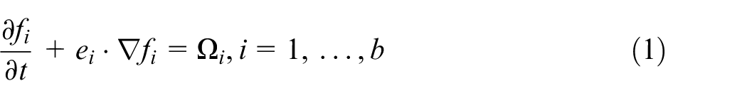
\frac{\partial f_{i}}{\partial t} + e_{i} \cdot \nabla f_{i} = Ω_{i}, i = 1, \dots, b

(1)

Where f_i is the particle distribution function in the direction i, e_i is the corresponding discrete velocity and Ω_i is the collision operator.

Turbulence modeling based on LBM solver is achieved using the Large Eddy Simulation (LES). This scheme introduces an additional viscosity, called turbulent eddy viscosity v_t, to model the sub-grid turbulence. The LES scheme in this current study is the Wall-Adapting Local Eddy viscosity model, that provides a consistent local eddy-viscosity and near wall behavior.³⁶ The actual implementation is formulated as follows:

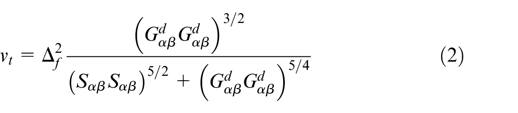
v_{t} = Δ_{f}^{2} \frac{{(G_{α β}^{d} G_{α β}^{d})}^{3 / 2}}{{(S_{α β} S_{α β})}^{5 / 2} + {(G_{α β}^{d} G_{α β}^{d})}^{5 / 4}}

(2)

Where Δ_f= c_wΔx is the filter scale, S is the strain rate tensor of the resolved scales and the constant C_w is typically 0.325.

In order to reduce computing needs for the flow field parameters nearby walls, XFlow uses a wall function to estimate the velocity nearby the wall, and the wall function to estimate the velocity is defined as follows³⁷:

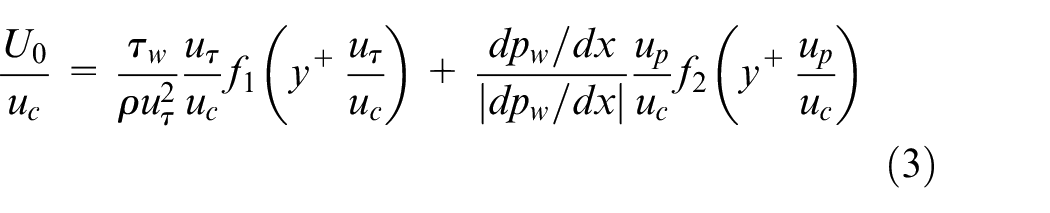
\frac{U_{0}}{u_{c}} = \frac{τ_{w}}{ρ u_{τ}^{2}} \frac{u_{τ}}{u_{c}} f_{1} (y^{+} \frac{u_{τ}}{u_{c}}) + \frac{d p_{w} / dx}{| d p_{w} / dx |} \frac{u_{p}}{u_{c}} f_{2} (y^{+} \frac{u_{p}}{u_{c}})

(3)

Here, y⁺ is the wall normal distance, u_τ is the skin friction velocity, τ_w is the turbulent shear stress, dp_w/dx is the wall pressure gradient, u_p is a characteristic velocity of the adverse wall pressure gradient and U₀ is the mean velocity, f₁ and f₂ are the interpolating functions.

It is strongly recommended to use the non-equilibrium enhanced wall-function for aerodynamic applications, since the prediction of the boundary layer separation based on pressure gradients is a fundamental feature. It sets the generalized wall function and takes into account for the pressure gradients to predict flow separation. Based on the inlet speed (U_f= 40 m/s) and the height H of Ahemd model, the Reynolds number was approximately 2.78 × 10⁶. The simulation time in total was 0.5s and the time step Δt=7.69231 × 10⁻⁵s is automatically estimated to ensure the numerical stability.

Data processing

For the convenience of comparison analysis, the time-averaged drag coefficient (C_D), pressure coefficient (C_P), slipstream velocity coefficient (U), and space velocity coefficient (u_l) were nondimensionalized as follows:

C_{D} = \frac{F_{D}}{\frac{1}{2} ρ U_{f}^{2} S}

(4)

C_{P} = \frac{P - P_{0}}{\frac{1}{2} ρ U_{f}^{2}}

(5)

U = \frac{\sqrt{{(U_{f} - U_{x})}^{2} + U_{z}^{2}}}{U_{f}}

(6)

u_{l} = \frac{U_{local}}{U_{f}}

(7)

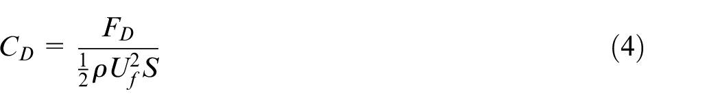
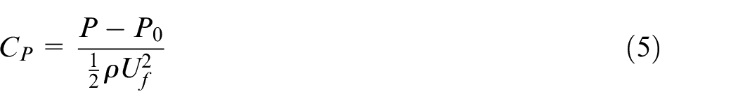
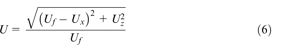
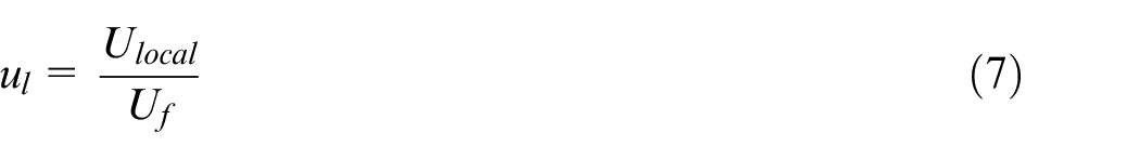
Where F_D is the aerodynamic drag, ρ is the air density (=1.225 kg/m³), and P₀ is reference pressure with 0 Pa; P represents the time-averaged static pressure on the car model surface; U_x and U_y represent the wind speeds in the streamwise and transverse components, respectively; U_local is the space wind speed around model, and U_f is the inlet speed equal to 40 m/s; the full-scale reference area S of the Ahmed model is 0.112 m².

Grid generation

XFlow is a particle based on lattice Boltzmann method (LBM) dynamics solver and the lattice structure has the characteristic of adaptability. Due to the presence of the rotation wheel, the flow field status around the wheel will change and then the lattice resolution changes dynamically to adapt to the flow patterns. The lattice adaptive refinement feature is based on the module of the vorticity field, which can effectively capture the changes of the flow field in the wake and the near wall.³⁸ Besides, three resolutions are required for fluid field calculation: the far field, the wake and the near wall resolutions.

In order to investigate the different lattice resolution sensitivity, three resolutions of the Ahmed body surface are generated, and the details of the three resolutions are shown in Figure 4. The resolution of the far field h was taken constant as 0.08 m, while that of the wake and the near wall of coarse, medium and fine resolutions are h/2², h/2³, and h/2⁴, respectively. In order to fully cover the turbulence flow, as shown in Figure 5(a), there are three refinement zones from fine resolution at the walls to coarse resolution in the far field, and each refinement zone is covered by four layers of grid. Figure 5(b) and (c) show the enlarged view of the front end and the rear end of the Ahmed body using the fine resolution.

Figure 4.

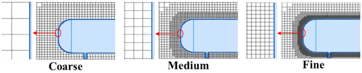
Different computational grids around the Ahmed body.

Figure 5.

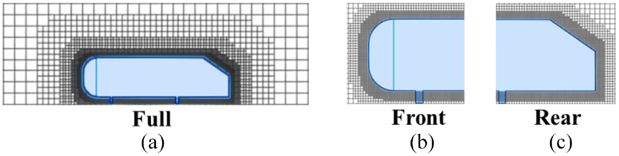
Fine grids around the Ahmed body: (a) global view and (b and c) local view of the front and rear.

Numerical validation

Figure 6(a) shows the convergence curves of aerodynamic drag coefficient based on three resolutions. It could be seen that the numerical results reached a steady state at time T1 = 0.3s, and the average value of drag coefficient between T1 = 0.3 s and T2 = 0.5 s was taken as the numerical result of the drag coefficient of Ahmed body. The time-averaged drag coefficients under different resolutions were compared with the experimental value by the work of Meile et al.,³⁹ as shown in Figure 6(b), the errors were 27.60%, 1.79%, and 2.87%, respectively. Moreover, the numerical error of the medium resolution was the smallest.

Figure 6.

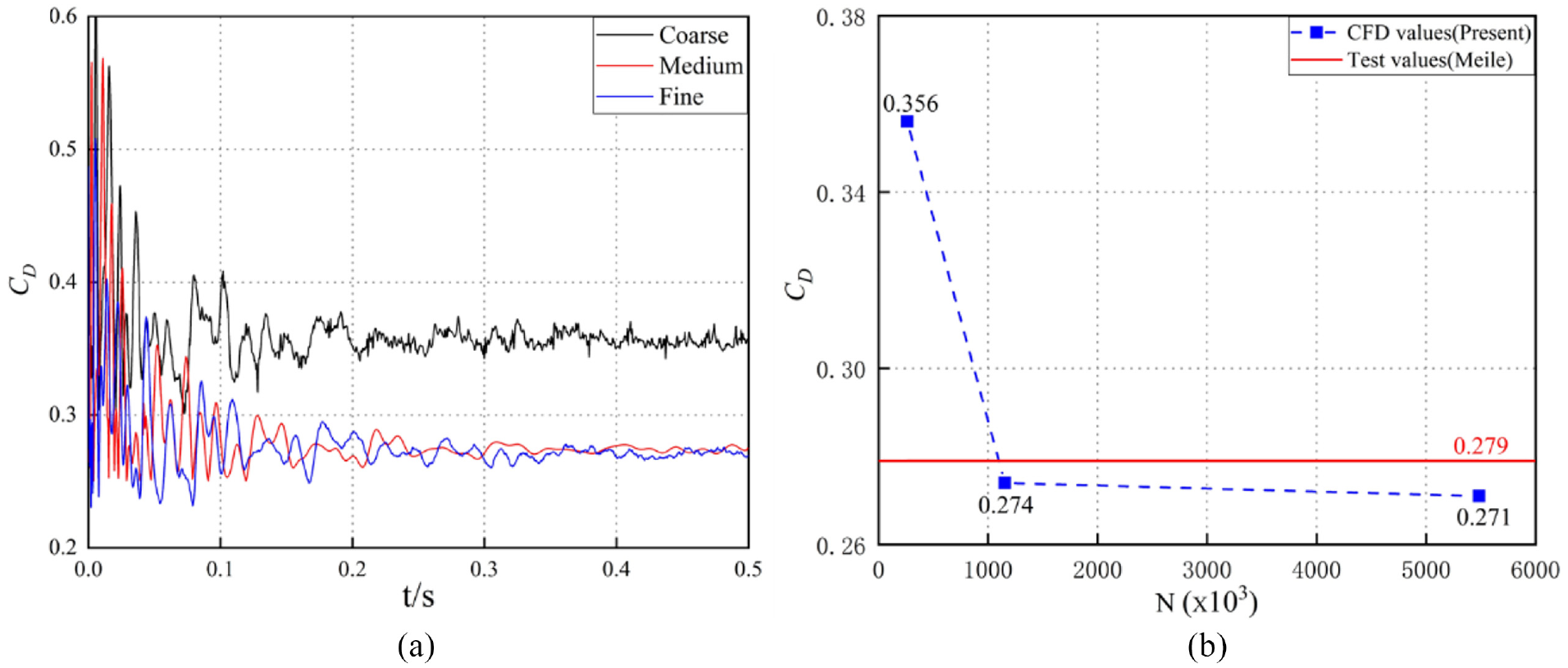
Comparison of different resolutions: (a) time histories of the aerodynamic drag of the Ahmed model and (b) the drag coefficient comparison between simulation and experiment.

To further verify the accuracy of the numerical methods, in Figure 7, the streamwise velocity profiles along the rear part of the Ahmed body obtained in this study were compared with experimental data measured by Lienhart et al.⁴⁰ The comparison showed good agreement between this numerical simulation and that experimental work. There were some minor deviations of drag and streamwise velocity profile between simulation and experiment which was reasonable, given the low values of velocity and the high turbulence that may impact experimental measurements.⁴¹ Thus, the LES method based on LBM solver can be used to analyze the aerodynamic characteristics of the Ahmed body and then the feasibility of the method was further studied.

Figure 7.

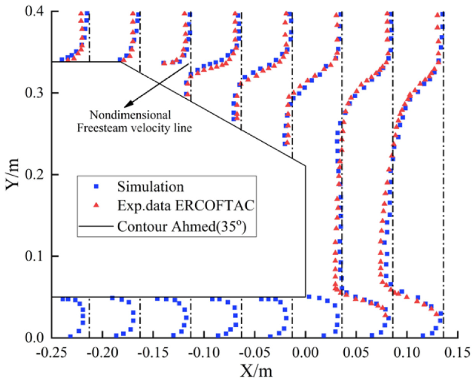
Comparison of velocity profiles between simulation and experiment.

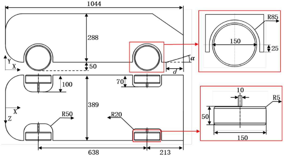
The typical features of the wheels and wheelhouses employed in this work are proportional to those of a real car with tires of 255/35 R19, which has the overall dimensions in same ratio as Ahmed body, as presented in Figure 8. The following parameters were considered for the wheels with a fully cover rim: outer diameter of the wheels is 150 mm, the height between axle and ground is 75 mm, the width of the wheels is 50 mm, the wheels track is 638 mm, the depth of the front wheelhouse and the rear wheelhouse were 100 and 70 mm, respectively. The ground clearance of the car body is h = 50 mm, and the center of the rear wheel was 213 mm away from the rear end. The wheels were mounted to the car body with a cylindrical axles of the diameter of 10 mm. An underbody diffuser was also considered, defined by diffuser length (d) and diffuser angle (α).

Figure 8.

Sizes of Ahmed dody with underbody diffuser and wheels.

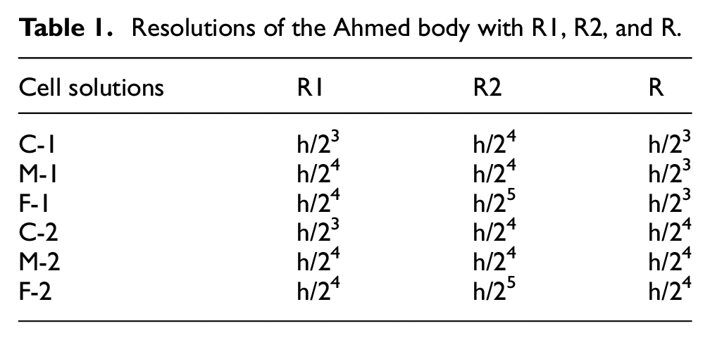
It was because the wheel has significant effects on the unsteady flow and wake vortex around the body, two refinement regions named as R₁ and R₂ were applied nearby the body and wheel, as shown in Figure 9. The size of the R₁ was 2H × 0.5H × 0.5H, while that of the R₂ was 0.18H × 0.18H × 0.5H. Using the wake and the near wall resolutions determined by the above verification, combined with resolutions of the refinement regions, the resolution scheme applicable to the simulation were further explored. The resolutions of different regions were shown in Table 1, where the h = 0.08 m was the far field resolution, and R was defined as the wake resolution using R = h/2³ and R = h/2⁴.

Table 1.

Resolutions of the Ahmed body with R1, R2, and R.

Cell solutions	R1	R2	R
C-1	h/2³	h/2⁴	h/2³
M-1	h/2⁴	h/2⁴	h/2³
F-1	h/2⁴	h/2⁵	h/2³
C-2	h/2³	h/2⁴	h/2⁴
M-2	h/2⁴	h/2⁴	h/2⁴
F-2	h/2⁴	h/2⁵	h/2⁴

Figure 9.

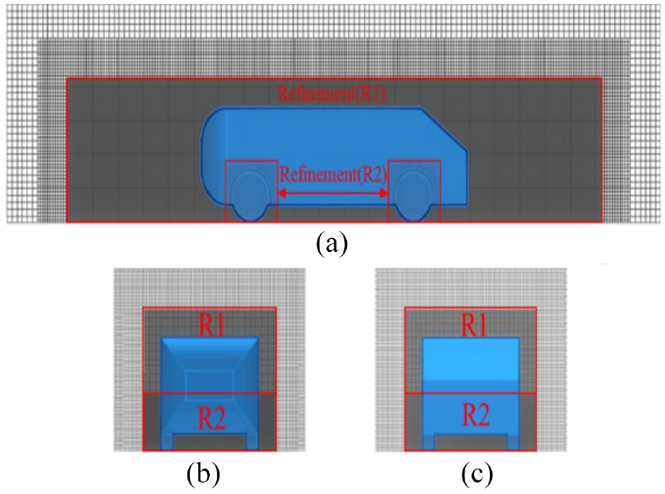
Grid around the Ahmed body with wheels, wheelhouse and underbody diffuser (d=0, α=0°): (a) side view, (b) front view, and (c) back view.

The Enforced mode was selected in the motion module of XFlow, and the motion type of Euler angles, for prescribed rotation around global axes, was used to simulate wheel rotation, and the angular velocity of wheels were defined as follows: X = 0, Y = 0, Z = 360 nt, which represents a rotation around the Z-axis in local coordinate system of the wheel, and n was the rotating speed of the wheel equal to 84.88 rps. Considering the complexity and unsteady flow around the rotation wheel, the simulation time in total was set to 2 s. The first part was the transient calculation to get the drag coefficient curve reaching a steady state at T = 1 s, and then in second part, the averaging of the fields was calculated during 1–2 s to filter the temporal fluctuations and to identify the main wake structures.

Figure 10 shows the numerical results according to different resolution schemes compared with the study of Huminic and Huminic.⁴² When the underbody diffuser length d = 0 and the angle α=0°, as shown in Figure 10(a), it could be seen that further refinement of the wake resolution had little effect on the results, but the level of the refinement resolution of the body and wheel regions had a greater impact on the results, and the smaller the resolutions in the refinement regions, the closer the numerical results were. Therefore, the resolution scheme F-1 was selected for further verification. After then, the drag coefficients of the five model configurations were studied under the conditions of the length d = 0.2H and the angle α = 1°, 3°, 5°, 7°, 9°, and Figure 10(b) shows that the calculation results using the resolution scheme F-1 were in good consistent with the study results conducted by Huminic, and the influence trend of the diffuser angles change on the model drag was similar. So the Ahmed body with diffuser length d = 0.2H and diffuser angle α = 5° was selected in current study, in which the drag coefficient was the lowest.

Figure 10.

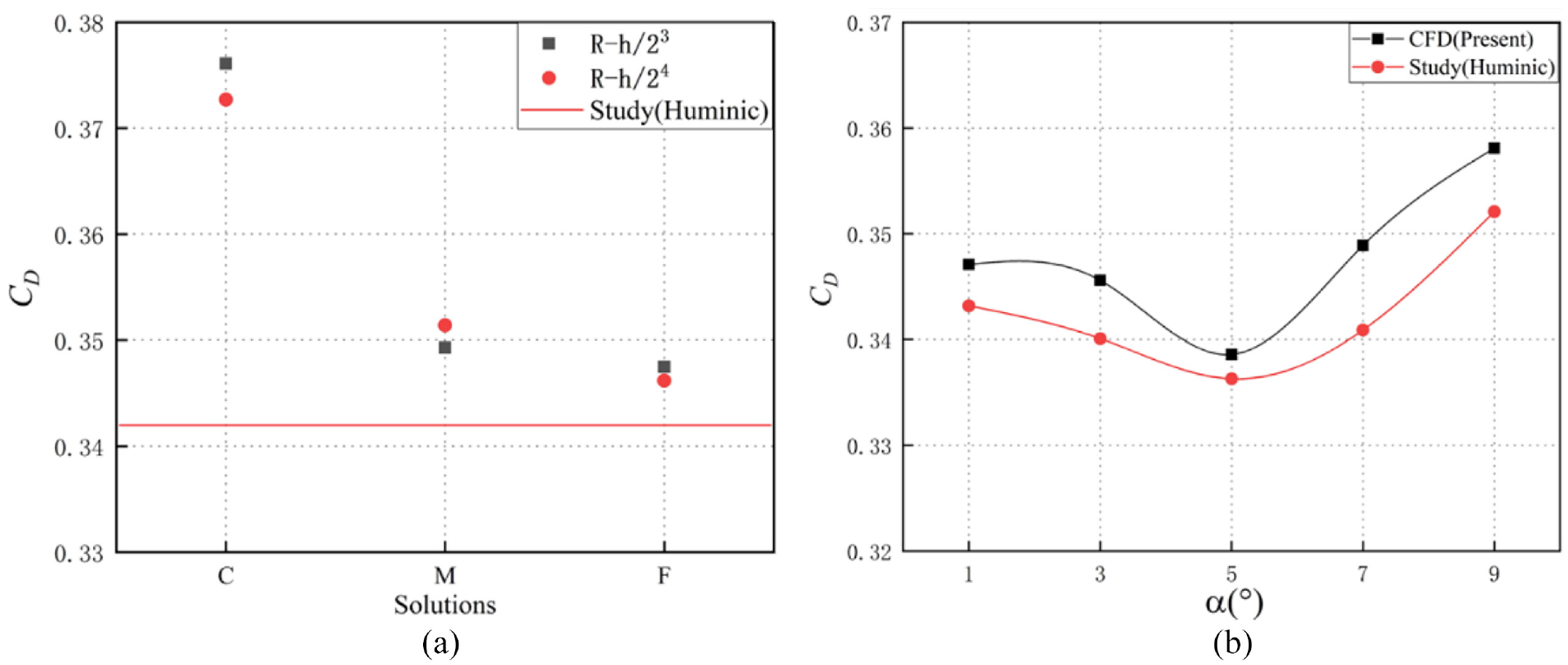
Comparison of the drag coefficient: (a) d = 0, 0° and (b) d = 0.2H, α = 1°, 3°, 5°, 7°, 9°.

As shown in Figure 11(a), the influences of wheel cavity cover on aerodynamic characteristics were studied by TUDelft university.⁴³ The geometrical parameters of wheel configurations include the upper and lower limits of wheel radial diameter, and the different opening area ratios of 50%, 70%, and 90% were obtained by changing the upper and lower limits of wheel radial diameters. Inspired by this wheel design method for the different ratios, a wheel with different opening areas was realized by changing the spoke angle under the conditions of the same outer diameter, the width and edge chamfering. Figure 11(b) shows the upper and lower limit of spoke diameter is 120mm and 30mm, and the thickness of spoke is 20 mm. The angles of adjacent spokes were respectively defined as 10°, 20°, 30°, 40° to get the different ratios of opening area. 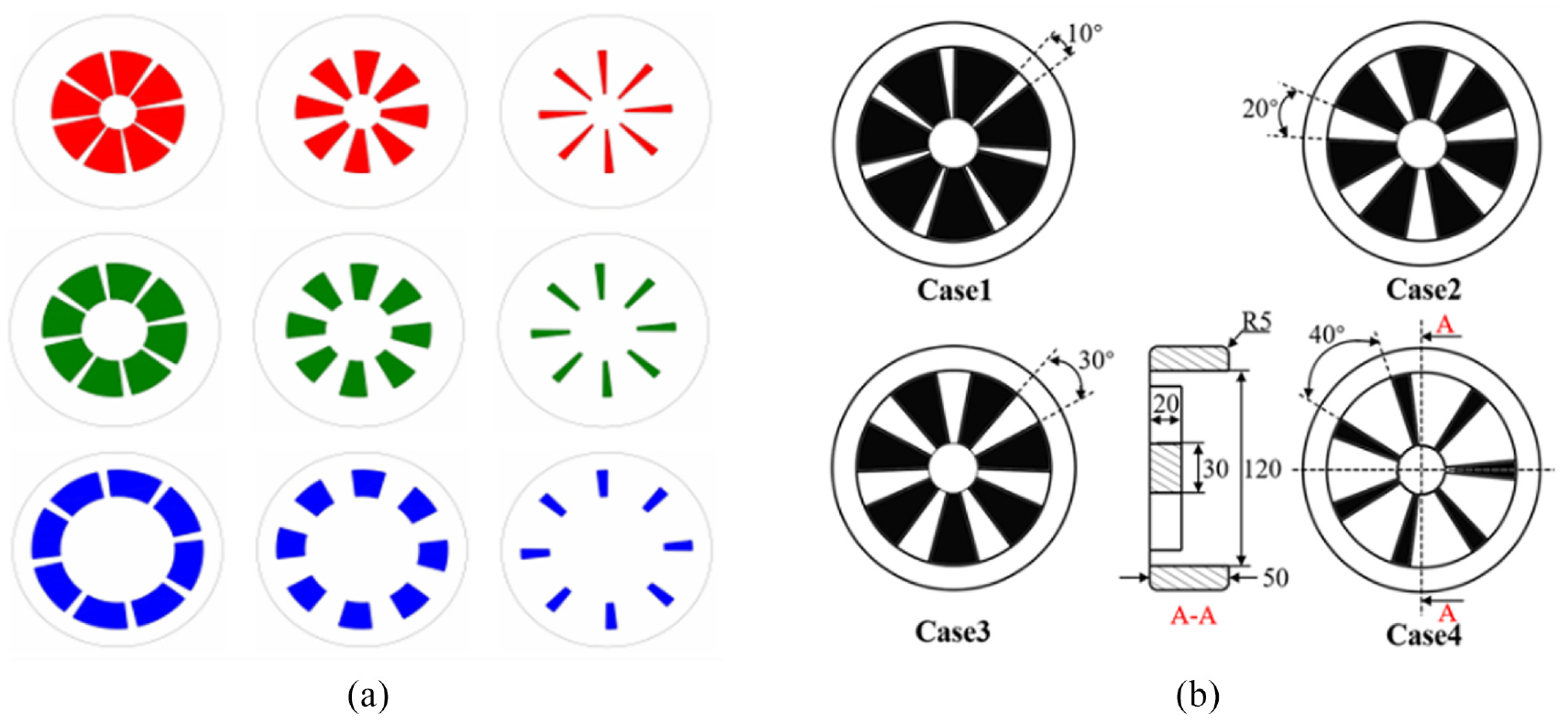Under the condition of not changing other simulation parameters, the best resolution scheme F-1 (R = h/2³, R1 = h/2⁴, R2 = h/2⁵) was selected for simulation calculation.

Figure 11.

Wheel configurations: (a) coverage area and radial placement of openings and (b) rim design geometrical parameters.

Results and discussion

The different wheel configurations have great influence on the aerodynamic characteristics, and in order to study the flow field and wake vortex around the wheel and car body, seven sections along the X-axis were selected as feature planes, and Figure 12 shows the detailed locations.

Figure 12.

Locations of seven sections in the cases.

Aerodynamic drag

The aerodynamic drag coefficients acting on the car model and different wheel configurations are shown in Figure 13. In order to contrast and analysis, the bodywork, front wheel and rear wheel of the car model were defined as BW, FW, and RW, respectively. As observed from Figure 13(a), with the increase of the rims opening area, the C_D values gradually increased from Cases 1 to 3, and then decreased from Cases 3 to 4. Besides, the C_D of Case 3 was largest among all cases, followed by Case 4 and Case 1 was the smallest.

Figure 13.

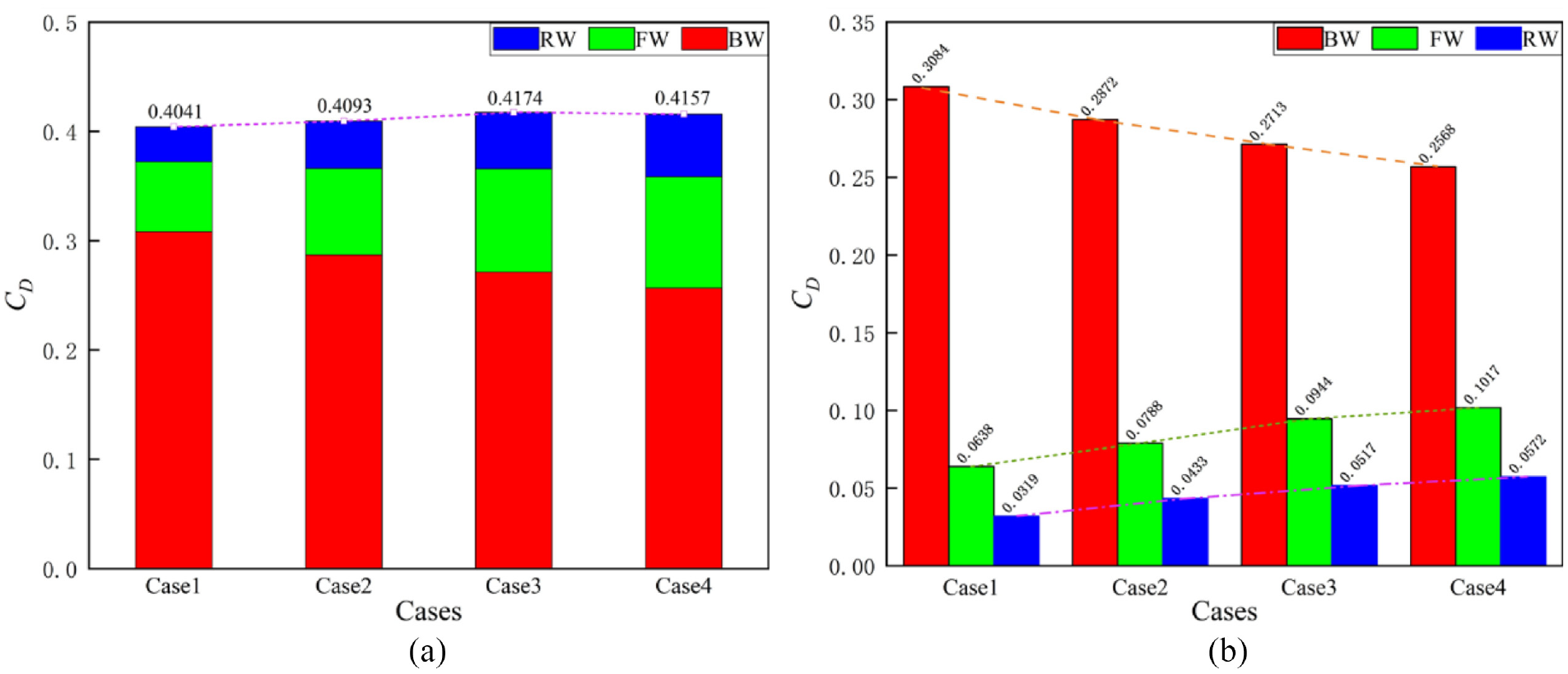
Time-average drag coefficient for each wheel configuration: (a) CD of the car model, and (b) CD of bodywork (BW), and front wheel (FW), and rear wheel (RW).

In order to better understand the aerodynamic behavior, Figure 13(b) shows the C_D of bodywork, front wheel and rear wheel. As the figure showed, the drag coefficient of BW gradually decreased from Cases 1 to 4, while the drag coefficients of FW and RW increased strictly, as the opening area increased, and the drag coefficient of the FW was larger than that of the RW. In other words, the front wheel configurations had greater influences on the aerodynamic drag of the car model than the rear wheel. As the opening area of rims increased, more airflow entered the wheel cavity and merged with the air flow from the bottom of the car, which strengthened the intensity and the energy dissipation of the vortex in the wheel cavity. The complex flow characteristics around the wheels leaded to the increase in the drag of the front and rear wheels. When the opening area was further increased, the velocity of the air flow into the wheel cavity increased, which interfered with the formation of the vortex in the wheel cavity, and brought part of the air flow out of the wheel cavity from the inside of the wheel, thus reducing the energy dissipation of the bodywork vortex and reducing the resistance of the car model.This maybe the reason why the C_D of Case 3 was larger slightly than Case 4.

As for the whole model, the C_D values of Case 1, Case 2, Case 3, and Case 4 were 0.4041, 0.4093, 0.4174, and 0.4157, respectively. And the largest C_D value in Case 3 was about 3.19% higher than least in Case 1. For further investigation on the contribution ratio of each component to the aerodynamic drag, the pie chart shows the detailed ratios of the C_D values of BW, FW and RW in Figure 14. As the opening area of the rim increased, the ratio of the drag coefficient of BW decreased sequentially at 6.15%, 5.17%, and 3.22%, while the proportion of the drag coefficient of FW increased sequentially at 3.46%, 3.37%, and 1.84%, and that of RW increased sequentially at 2.69%, 1.81% and 1.39%, respectively. The order of contribution ratio of each component to the vehicle drag was the similar among all cases, as follows: BW > FW > RW. Compared with the closed wheel configuration, the open wheel configurations may have a greater influence on the vehicle drag. It can be inferred that when the opening area of rim increases in equal proportions, the drag coefficient of the car model did not increase linearly.

Figure 14.

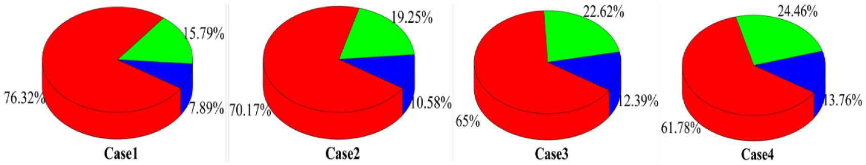
Proportions of drag coefficient of BW in red, FW in green and RW in blue.

Flow fields around the car model

To better investigate the effect of different wheel configurations on the aerodynamic drag, the distribution of the mean surface pressure acted on the car surface is shown in Figure 15. As shown in Figure 15(a), the front end of the blunt head had a positive pressure under the action of the airflow. As the air flowed along the blunt head, the surface pressure dropped significantly, and a large area of negative pressure appeared, and then the surface pressure gradually increased. It could be seen that in all cases the surface pressure distribution in the front-end region of the car body was almost the same. The airflow passes more smoothly through the front of the car body due to its inverted round, which means that the front end encounteres less airflow impact, thus a large negative pressure area appears around the front surface. The length of the negative pressure area on the upper surface of the middle bodywork was different, and the length of the negative pressure area of Cases 2 and 3, defined as L2 and L3, were similar, but smaller than that of Case 1 and larger than that of Case 4. Besides, there was an obvious difference in the surface pressure distribution in the slant, and the pressure value decreased, which leads to the increase of the pressure drag of the model from Cases 1 to 4. There was a higher pressure area and a higher positive pressure value on the lower surface of the blunt front than on the upper surface, and then a small area of low pressure nearby the front wheel appeared on the lower surface, but the low pressure area in Case 1 was larger and more obvious in all cases in Figure 15(b). Moreover, the lower surface pressure of the middle bodywork increased gradually along the direction of the model body, and a higher-pressure value appeared nearby the rear wheel. Although the high pressure area of Case 4 was smaller than that of Cases 3 and 2, the overall pressure value was larger, and then the pressure in the tail area decreased significantly. The difference in the pressure distribution fully proves that the variations of drag coefficients are the results of changes in flow field characteristics.

Figure 15.

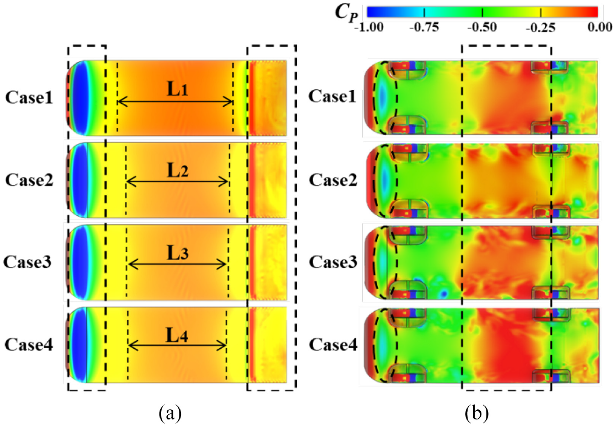
Mean surface pressure on the model: (a) the upper and (b) the lower.

Figure 16 shows the mean pressure along the upper and the lower centerline of the car model. The pressure on the upper surface was similar shown in Figure 16(a) and (b), although the front pressure of the blunt fluctuated in a small range, the changing trend was still consistent, which was mainly caused by the interaction of airflow along the front and horizontal airflow. It was obvious that the pressure fluctuation of the slant of the model was quite different, in which the pressure distribution of Cases 3 and 4 were significantly lower than that of Cases 1 and 2, which could also be observed in Figure 15(a). As shown in Figure 16(c), in contrast, the pressure on the lower surface of the car model was more volatile and was greatly affected by the wheel configurations. On the lower surface of the front end, the pressure amplitude of Cases 1 and 2 was lower than that of Cases 3 and 4. The pressure along the lower centerline between the front and rear wheel increased at first and then decreased gradually, and the fluctuating trend of all cases was similar, in which Case 4 had the highest volatility, while that of the Case 1 was the smallest, which indicated that the surface pressure distributions on the lower surface were obviously affected by the wheel configuration with different opening area.

Figure 16.

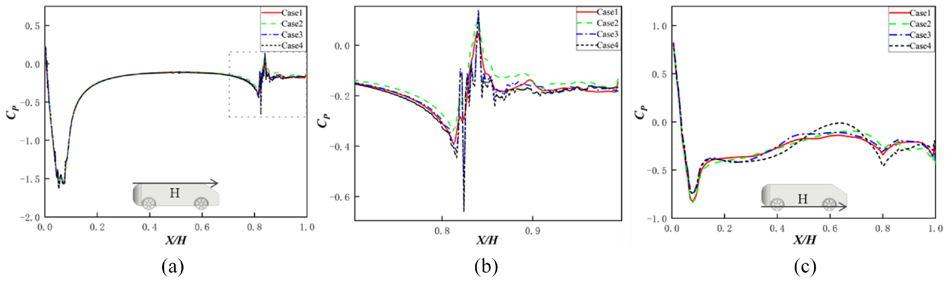
Mean pressure along the centerline of the model: (a) the upper, (b) enlarge view and (c) the lower.

To analysis the evolution of the flow vortices in the instantaneous flow field around the car with different wheel configurations, the second invariant, Q criterion, for the velocity gradient tensor.⁴⁴ The Q criterion is defined as follows:

Q = - \frac{1}{2} (S_{ij} S_{ij} - Ω_{ij} Ω_{ij})

(8)

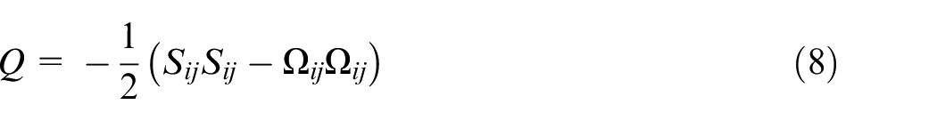
Where, Ω_ij is the rotation tensor and S_ij is the strain rate tensor; Ω_ij and S_ij are the anti-symmetric and symmetric parts of the velocity gradient, respectively.

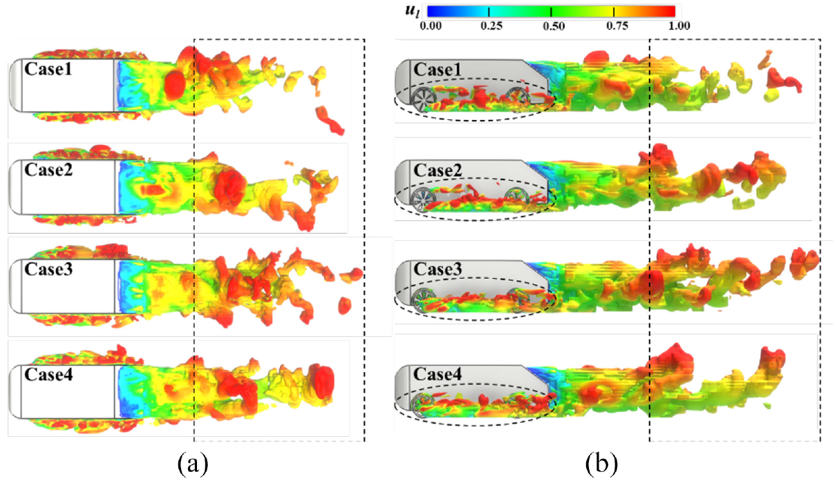
As shown in Figure 17(a), the wheel configurations has a great influence on the aerodynamic behavior. The vortex structures around the wheel were different in all cases, although the width of the vortices of the Case 3 was only slightly smaller than that of the Case 4, the relationship in all cases was as follows: W₄> W₃> W₂> W₁. This was mainly due to the increase in the opening area of rims, which leaded to complex flow separation around the wheel and produced a wide range of vortices, and this may also be the reason for the increase in drag of the front and rear wheel. Meanwhile, it was important to note that there was also a difference in the wake and it could be seen that the wake vortex of Cases 3 and 4 were larger than that of Cases 1 and 2, this difference could also be observed in Figure 17(b). The height of trailing vortices in Case 1, defined as H₁, was lowest of all cases, which implied that there was a small range of vortex breaking and shedding in the wake of Case 1, whereas that of other cases led to the larger flow fluctuations.⁴⁵ Although the height of trailing vortices in Cases 2–4 were relatively close, the wake vortex in Case 3 was larger and the flow was more complex than the other two cases, which also may lead to the greatest drag in all cases, and at the same time, the vortex shedding occurred in the wake in Case 4. As observed from Figure 17(b), the flow vortices were generated continuously, and they propagated from the bottom to the top and rear of the model. We could also see that large differences were found in the development of the flow vortices in all cases around the bodywork, the vortices created by airflow over the front wheels moved backward along the flow direction. Gradually, the flow field around the car model became more complex and disordered, thus forming a larger number of vortices in the wake region as a result of the separation in the attached boundary layer, and the airflow velocity was reduced in the region near the tail.

Figure 17.

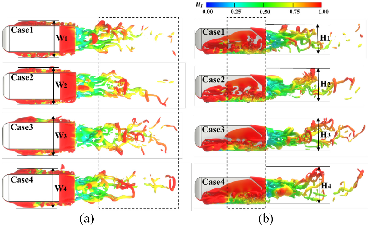
Instantaneous iso-surfaces coreesponding to the criterion (Q = 60,000), rendered for the time-averaged space velocity: (a) top view and (b) side view.

The iso-surfaces of instantaneous turbulence intensity, which are colored using the time-averaged space velocity, are visualized in Figure 18, and the turbulence intensity I (in %) is defined as follows:

I = \frac{u'}{U}

(9)

Figure 18.

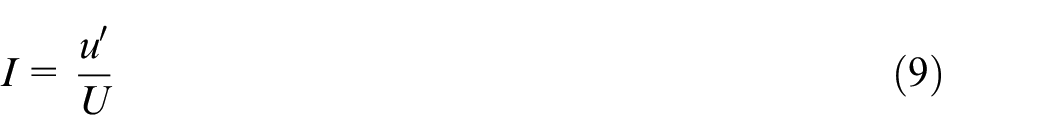
Instantaneous iso-surfaces of the turbulence intensity, rendered for the time-averaged space velocity: (a) top view and (b) side view.

where the µ′ is the root-mean-square of the turbulent velocity fluctuations, and which can be described as:

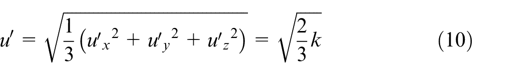
u' = \sqrt{\frac{1}{3} ({u'}_{x}^{2} + {u'}_{y}^{2} + {u'}_{z}^{2})} = \sqrt{\frac{2}{3} k}

(10)

Here the k is the turbulent kinetic energy, while the U is the mean velocity and which is computed from the three mean velocity components.⁴⁶

As shown in Figure 18(a), the turbulence intensity in the wake and wheel regions were relatively large. Among all the cases, the turbulence intensity in the wake of Case 3 was the largest, and while that of Case 1 was the smallest, and there was some difference between Case 2 and 4, but Case 4 was larger than Case 2. This phenomenon could be also observed in Figure 18(b). The change in the turbulence intensity in the wheel region was more obvious. Due to the increase in the opening area of rims, the turbulence intensity in the front wheel region became larger gradually, and moreover, this effect adverted backward along the model, result in a higher turbulence level in the rear wheel region in all cases. Increasing the opening area would aggravate flow unsteady around the bodywork, and it has a direct influence on the wake vortex flow. The fluctuation of the flow in the wake and wheel regions affected the change of the drag of the car model, in which the wake pressure decreased and the pressure drag increased. There was a higher level of turbulence intensity in the wake of Case 3, which may be the most possible causes for the greatest drag of the Case 3 in all cases.

The aerodynamic drag of the car model consists of two parts: pressure drag and viscous drag, and the previous sections provided an analysis of the pressure distribution and flow structures. While the viscous drag depends mainly on the the boundary layer thickness.⁴⁷ The boundary layer thickness, defined as the wall-normal distance from the position of 0.99U_f to the model wall, has been commonly used to explore the near-wall flow field. As demonstrated in Figure 19(a), along the length direction of the model body, the boundary layer thickness increased gradually, and there was a slight discrepancy in the boundary thickness of the front end and the middle of the bodywork. Due to the more complex flow in the wake, there was a certain difference in the boundary layer thickness. Figure 19(b) shows the boundary layer thickness of the horizontal plane at Y = 0.075 m in the width direction, which passes through the center of the front and rear axles. Compared with Figure 19(a), the difference in the width direction of the boundary layer among the four cases was greater than that in the length direction, especially in the front wheel regions and the wake, as shown in Figure 19(b). Moreover, the boundary layer thickness of Case 3 in the wake was slightly larger than that of Case 4, but both were larger than Cases 1 and 2, mainly due to the difference of the opening area in rims. In Figure 19(c), small differences could be observed in regions above a half height of the model, and the thickness of the boundary layer increased gradually from front wheel to rear wheel. However, in regions below a half height of the model, the boundary layer thickness was greatly affected by the wheel configurations, and the boundary layer thickness of Cases 3 and 4 were larger than that of Cases 1 and 2. The closer to the ground, the thicker the boundary layer, and the closer to the tail of the model, the more obvious the phenomenon. Because the boundary layer thickness is related to the aerodynamic drag, and a thicker boundary layer would result in a greater aerodynamic drag, the contour features of boundary layers could explain why the aerodynamic drags of Cases 3 and 4 were obviously higher than that of Cases 1 and 2.

Figure 19.

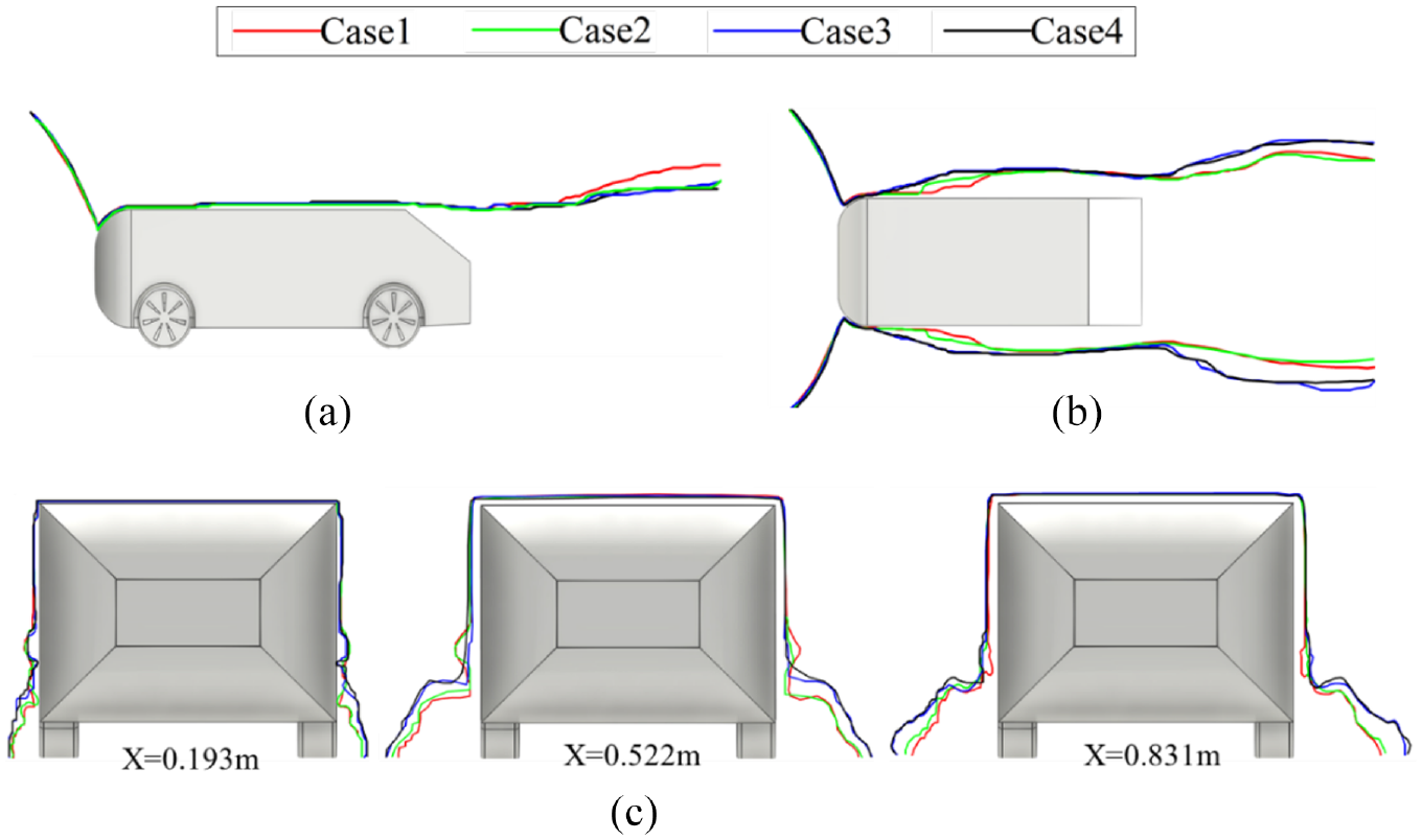
Boundary layer contour features:(a–c) are the symmetry plane at Z = 0, and the horizontal plane at Y = 0.075 m, and cross sections X = 0.193 m, 0.522 m, and 0.831 m, respectively.

To study the effects of different wheel configurations on the flow distribution in the wake, the time-averaged streamlines in the symmetry planes and the vertical planes at 0.1, 0.2, and 0.4 m away from the rear back are presented in Figure 20. As demonstrated in Figure 20(a), the vortex structure mainly consists of the flow separation zone V1 of the slant and two recirculation areas V2 and V3 in the wake, one at the junction of the slant and the vertical rear back, while the other close to the vertical rear back and the center of the vortex core was closer to the ground. The vortex V1 can be observed more obviously in Case 4, and the position was closer to the lower edge of the slant than that of other cases. The incoming flow at the bottom of the model flowed to the wake along the underbody diffuser, due to the influence of the low pressure in wake, part of the air flow flowed upward, and then form a vortex V2 with the incoming flow at the top of the model. The vortex V2 was more obvious in Cases 3 and 4. Similarly, the incoming flow at the top of the model was subjected to the entrainment of the low pressure at vertical rear back, forming a larger recirculation area V3. Unlike the vortex V2, the vortex core and vorticity of the vortex V3 were larger and could be clearly observed in all cases. In Figure 20(b), in the vertical planes behind the model, a pair of the opposite helical cylindrical vortexes can be observed obviously, especially in the vertical plane X1 = 0.1 m. Although the center distance d3 of the vortex core in Case 3 was the shortest in all cases, the vorticity near the vortex core was larger than Case 4. Moreover, the center distance d2 and d4 of the vortex core in Cases 2 and 4 were similar, but both were larger than that in Case 1. The farther away from the back of the model, the effect of the spiral cylindrical vortex was gradually weakened, and then the vortex shedding and separation occurred.

Figure 20.

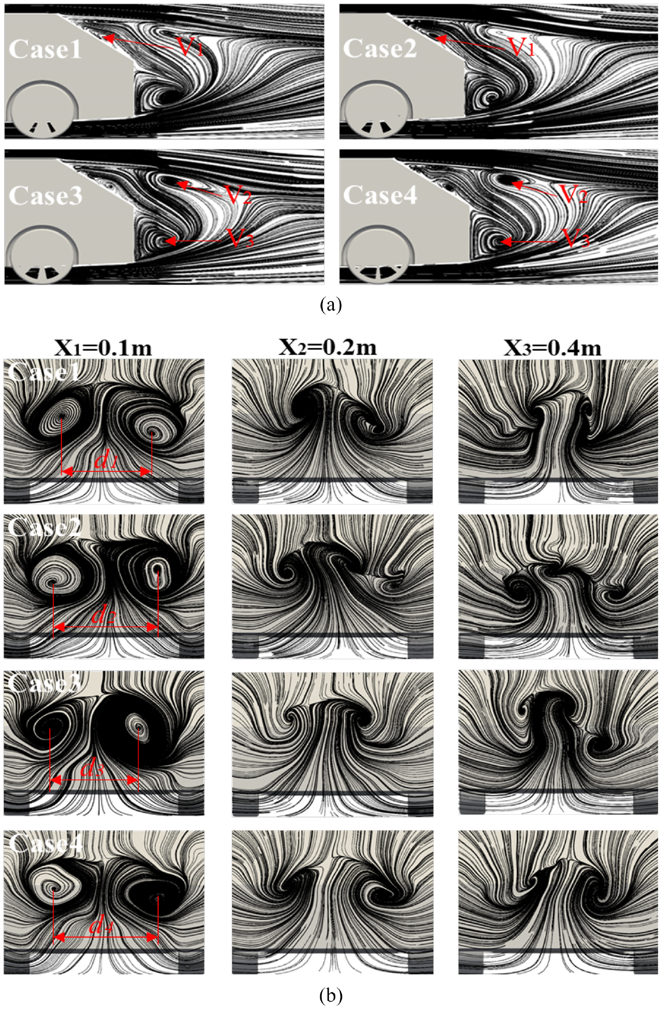
Time-averaged streamlines distributions: (a) streamlines in the symmetry planes and (b) streamlines in the vertical planes at 0.1, 0.2, and 0.4 m from the vertical rear back, respectively.

Slipstream and vorticity profiles

In this study, the first part of computational process was transient calculation, and there were only instantaneous results data to output. After the convergence of flow fields reaches a relatively steady state, the time-average of the unsteady flow-fields were calculated and output in second part, and the time-averaged values of slipstream velocity coefficient U were obtained at various distances from the Y-axis and Z-axis. Figure 21 presents the measurement positions, including four heights to the Y-axis and four distances to the Z-axis.

Figure 21.

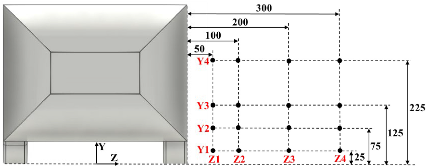
Location of slipstream in full-scale size (in mm).

The time-averaged slipstream profiles monitored at Y2 = 75 mm for various distances to the Z-axis are shown in Figure 22. In general, there was a obviously sharp peak of U around the front end in all cases, and this occurred because of the air pushing ahead and aside, results in a rapid acceleration in the airflow. As shown in Figure 22(a), the slipstream velocity between the front and rear wheels fluctuated greatly and there were great differences. At First, the slipstream velocity in all cases reduced rapidly. When the slipstream velocity of Cases 1 and 2 reached the trough, there was a small range of fluctuations, and then gradually increased. The difference was that the slipstream velocity of Cases 3 and 4 increased rapidly after reaching the minimum value, the peak value of Case 3 was higher than that of Case 4.

Figure 22.

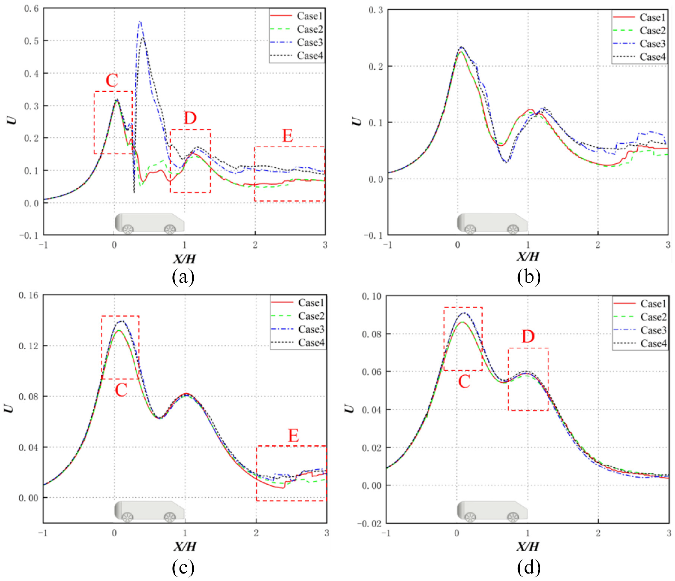
Time-averaged slipstream at Y2 = 75 mm for different distances from the Z-axis: (a) Z1 = 50 mm, (b) Z2 = 100 mm,(c) Z3 = 200 mm, and (d) Z4 = 300 mm.

In Figure 22(b), the fluctuation of the slipstream velocity was not as obvious as in Figure 22(a). In contrast, the slipstream velocity between the front and rear wheels in all cases decreased and then increased, but there were lower values in Cases 3 and 4, and the slipstream velocity in the wake region were significantly higher than in Cases 1 and 2. However, in Figure 22(c), the fluctuation of slipstream velocity was further weakened and there was a small difference in all cases, except in the regions C and E. Moreover, with an increase in distance, the results showed a similar tendency in all cases and the profiles of each case gradually changes to a similar steady state, as demonstrated in Figure 22(d), although there was still a small difference in region C at the front of the model, the peaks of Cases 3 and 4 were slightly higher than those of Cases 1 and 2. Along the airflow direction, the slipstream velocity first increased and then decreased gradually, then continued to increase, and reached a peak again in region D at the tail of the model, where the slipstream velocity gradually decreased in the wake region. As a result, due to the differences in wheel configurations, strong interference caused the airflow disturbance, and then further triggered greater fluctuations in slipstream velocity.⁴⁸

Figure 23 illustrates the time-averaged values of U at a distance of Z2 = 100 mm for different heights to Y-axis. As observed from the Figure 23(a), the slipstream velocity peaks of Cases 3 and 4 were larger in region C, and then decreased sharply and then increased rapidly, reaching a new peak. In contrast, the slipstream velocity of Cases 1 and 2 changed slowly and then reached a trough at X = 0.67H. Moreover, the values of slipstream velocity of Cases 3 and 4 were also higher than that of Cases 1 and 2 in regions D and E. However, in Figure 23(b), the slipstream velocity peaks were basically the same in region D in all cases, although the lowest values were different. With an increase in height to Y-axis, the change tendency of the slipstream velocity was same for each case and the profiles gradually coincides, except that there was still a small fluctuation in region E in the wake, as demonstrated in Figure 23(c) and (d). In addition, the fluctuation of U value gradually decrease in regions C and D with an increase in height, as shown in Figure 19, where the slipstream velocity shows a powerful correlation with the boundary layer thickness distribution around the car model.

Figure 23.

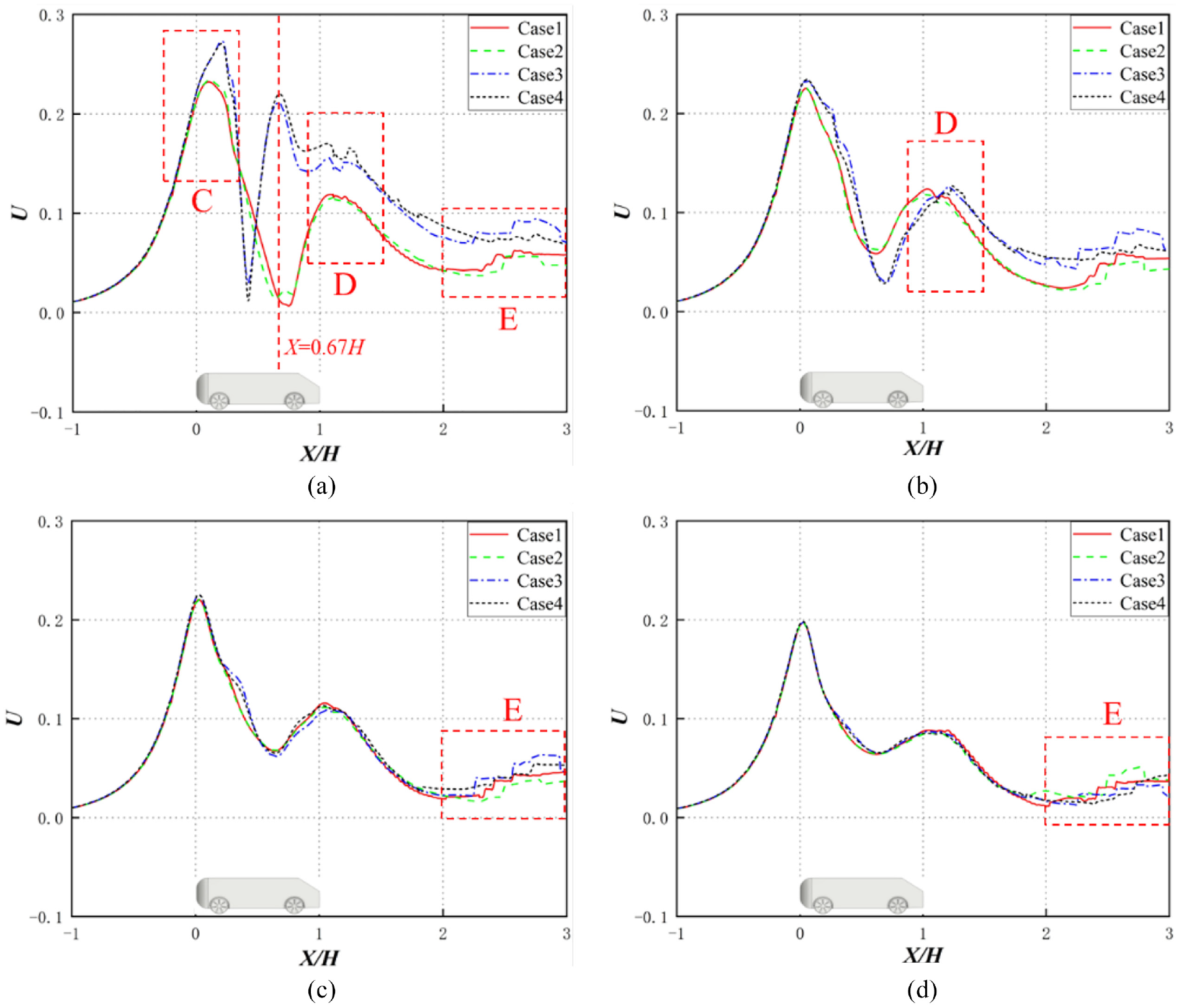
Time-averaged slipstream at Z2 = 100 mm for various heights from the Y-axis: (a) Y1 = 25 mm, (b) Y2 = 75 mm, (c) Y3 = 125 mm, and (d) Y4 = 225 mm.

In order to better explore the effects of the different wheel configurations on the flow around the bodywork, and then the following sections provided an analysis of the time-averaged velocity vectors and vorticity in four different cross-sections around the model in the flow direction, as shown in Figure 24. Due to the effect on the near-ground jetting vortex, the flow near the ground was directed away from the wheel with the increase in opening area, indicating that more air was flowing through the rims and feeding the jetting vortex, as demonstrated in Figure 24(a). In addition, there were three distinct regions V1, V2, and V3 of high vorticity at the front wheels, located at the wheel cavity, at the spoke opening, and near the ground, respectively. As the opening area of rim increased, the three high vorticity regions gradually melted together, indicating that the vorticity in the front wheel region further increased, especially in Case 4. The vortex further developed along with the bodywork and was affected by the airflow under the model, and there was still a high vorticity area on the side of the bodywork, which was most obvious in Case 3, and the high vorticity region was larger in Figure 24(b). While in Figure 24(c), two more obvious vorticity regions V4 and V5 were observed in the rear wheel area, located at the opening of the spokes and near the ground, of which V4 was more pronounced. Moreover, compared with the front wheels, the vorticity area V5 of the rear wheels near the ground was greatly reduced than V3, while the vorticity area V4 at the spoke opening was only reduced in a small range, which showed that the effects of the front wheel configurations on the aerodynamic characteristics of the car model was greater than that of the rear wheel. At the same time, this may be the reason why the aerodynamic drag of the front wheel is greater than that of the rear wheel, as shown in Figure 13. In the rear cross-sections of the car model shown in Figure 24(d), there were elongated regions V6 of high vorticity around the body surface, which could be observed in all cases. At this time, the airflow from the side of the model gradually flowes to the bottom of the model.

Figure 24.

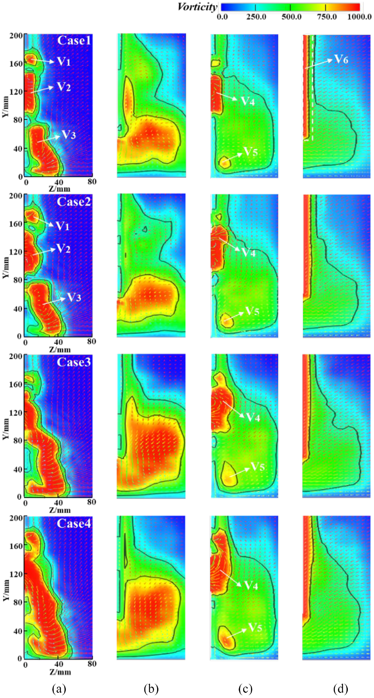
Time-averaged space velocity vectors and vorticity in cross-sections: (a) X = 0.193 m, (b) X = 0.522m, (c) X = 0.831 m, and (d) X = 1.044 m.

Conclusions

In this works, the combined method of LES and Lattice Boltzmann was used to explore the influence of wheels with different opening areas on the aerodynamic behavior of a general Ahmed model. The aerodynamic drag, the flow structures around the vehicle model and wheels, and the distribution of velocity and vorticity were analyzed. The conclusions of this study are summarized in three main points as follows:

The larger the opening area of rim within a certain range, the greater the drag of the car model, which could be approximated as a linear relationship. The drag of the front and rear wheel is a positive linear relation as rim opening area increases, whereas the drag of the bodywork is a negative relationship. Among all wheel configurations, the drag coefficient of Case 1 was the smallest, followed by Case 2, and the largest was Case 3, which was about 3.29% lower than the maximum drag coefficient of vehicle model.

The distribution and fluctuation of the pressure acting on the vehicle underbody were significantly affected by the wheel configurations, and there was a significant difference in the thickness of the boundary layer between the wheel region and the wake region, and the boundary layers of Cases 3 and 4 were quite thicker. Moreover, there was a larger turbulence level around the wheel region due to the increase of the opening area; the order of the vortices width in the wheel region was as follows: W₄> W3 > W2 > W1. Then the vortex further developes along the bodywork, which formes a higher concentration level and distribution area of turbulence intensity in the wake.

The slipstream velocity around the front and rear wheel firstly increased and then decreased, and the velocity fluctuation around the front wheel is more obvious than that of the rear wheel. The height and distance along the Y-axis and Z-axis increased, and then the effect gradually weakens, at the same time, the change in trends of all slipstream curves tends to a unified stead state. The vorticity of the front wheel region was larger than that of the rear wheel, and the increase in opening area results in the vorticity areas V1, V2, and V3 gradually connected to form a large area. The airflow in the region near the ground of the front wheel was far away from the wheel, while the airflow at the rear of the model gradually flowed along the sides to the underbody of the model.

Footnotes

Declaration of conflicting interests

The author(s) declared no potential conflicts of interest with respect to the research, authorship, and/or publication of this article.

Funding

The author(s) disclosed receipt of the following financial support for the research, authorship, and/or publication of this article: This study was financially supported by the National Natural Science Foundation of China (52072156) and the Postdoctoral Foundation of China (2020M682269).

ORCID iDs

Haichao Zhou

Qingyang Wang

Zhou Zheng

References

Holmberg

Andersson

Erdemir

. Global energy consumption due to friction in passenger cars. Tribol Int 2012; 47: 221–234.

Hucho

Sovran

. Aerodynamics of road vehicles. Annu Rev Fluid Mech 1993; 25: 485–537.

Siddiqui

N A

Chaab

M A

. A simple passive device for the drag reduction of an ahmed body. J Appl Fluid Mech 2021; 14(1): 147–164.

Hanfeng

Chao

, et al. Aerodynamic drag reduction of an Ahmed body based on deflectors. J Wind Eng Ind Aerodyn 2016; 148: 34–44.

Keogh

Barber

Diasinos

, et al. The aerodynamic effects on a cornering Ahmed body. J Wind Eng Ind Aerodynamics 2016; 154: 34–46.

Rao

Minelli

Basara

, et al. On the two flow states in the wake of a hatchback Ahmed body. J Wind Eng Ind Aerodyn 2018; 173: 262–278.

Faraj

Harika

Ramadan

, et al. Effect of underhood architecture on aerodynamic drag—suggestion of new concepts for fuel consumption reduction. Int J Autom Technol 2020; 21(3): 633–640.

Rüttgers

Park

You

. Large-eddy simulation of turbulent flow over the DrivAer fastback vehicle model. J Wind Eng Ind Aerodyn 2019; 186: 123–138.

Mlinaric

Sebben

. Investigation of the influence of tyre deflection and tyre Contact patch on CFD predictions of aerodynamic forces on a passenger car. In: Vehicle aeródynamics – 7th, MIRA international vehicle aerodynamic conference, Nuneaton, UK, 22–23 October; 2008.

10.

Wang

Zhang

, et al. Analysis and multi-objective optimization design of wheel based on aerodynamic performance. Adv Mech Eng 2019; 11(5): 1–19.

11.

Brandt

Berg

Bolzon

, et al. The effects of wheel design on the aerodynamic drag of passenger vehicles. SAE technical papers, 2019-01-0662, 2019.

12.

Chang

Ying

Yingchao

, et al. Influence performance with wheel spoke design parameters of vehicle aerodynamic. J Jilin Univy (Eng Techn Ed) 2021; 51(1): 107–113.

13.

Gleason

Duncan

Walter

, et al. Comparison of computational simulation of automotive spinning wheel flow field with full width moving belt wind tunnel results. SAE technical paper 2015-01-1556, 2015.

14.

Lounsberry

Gleason

Kandasamy

, et al. The effects of detailed tire geometry on automobile aerodynamics-a CFD correlation study in static conditions. SAE technical paper 2009-01-0777, 2009.

15.

Landström

Walker

Christoffersen

, et al. Influences of different front and rear wheel designs on aerodynamic drag of a sedan type passenger car. SAE technical paper 2011-01-0165, 2011.

16.

Wittmeier

Widdecke

Wiedemann

, et al. Tyre development from an aerodynamic perspective. ATZ Worldw 2013; 115(2): 42–48.

17.

Landstrom

Walker

Löfdahl

. Effects of ground simulation on the aerodynamic coefficients of a production car in yaw conditions. SAE technical papers, 2010 -01-0755.

18.

Landstrom

Josefsson

Walker

, et al. Aerodynamic effects of different tire models on a sedan type passenger car. SAE technical papers, 2012-01-0169, 2012.

19.

Tran

Anyoji

Nakashima

, et al. Experimental study of the skin-friction topology around the Ahmed Body in cross-wind conditions. J Fluid Eng 2022; 144(3): 1–11.

20.

Mercker

Breuer

Berneburg

, et al. On the aerodynamic interference due to the rolling wheels of passenger cars. SAE technical papers 910311, 1991.

21.

McManus

Zhang

. A computational study of the flow around an isolated wheel in contact with the ground. J Fluid Eng 2006; 128(3): 520–530.

22.

Koitrand

Lofdahl

Rehnberg

, et al. A computational investigation of ground simulation for a saloon car. SAE Int J Commer Veh 2014; 7(1): 111–123.

23.

Wang

Yin

Yan

, et al. Validation of aerodynamic simulation and wind tunnel test of the New Buick Excelle GT. SAE Int J Passenger Cars Mech Syst 2017; 10(1): 195–202.

24.

Guzman

Cho

Tripp

, et al. Further analyses on prediction of Automotive Spinning Wheel Flowfield with full width moving belt wind tunnel results. SAE Int J Passenger Cars Mech Syst 2017; 10(2): 600–618.

25.

Jia

Bao

, et al. A comparative study of different wheel rotating simulation methods in automotive aerodynamics. SAE technical paper, 2018-01-0728, 2018.

26.

Lee

M-H

Shiah

Bai

C-J

. Experiments and numerical simulations of the rotor-blade performance for a small-scale horizontal axis wind turbine. J Wind Eng Ind Aerodynamics 2016; 149: 17–29.

27.

Haag

Blacha

Indinger

. Experimental investigation on the aerodynamics of isolated rotating wheels and evaluation of wheel rotation models using unsteady CFD. Int J Automot Eng 2017; 8(1): 7–14.

28.

Schnepf

Schütz

Indinger

. Further investigations on the flow around a rotating, isolated wheel with detailed tread pattern. SAE Int J Passenger Cars Mech Syst 2015; 8(1): 261–274.

29.

Qingwei

, et al. Study on aerodynamic characteristic of vehicle with rotating wheels based on LBM. J Chongqing Univ Technol (Nat Sci) 2021; 35(6): 1–8.

30.

Hobeika

Sebben

. CFD investigation on wheel rotation modelling. J Wind Eng Ind Aerodyn 2018; 174: 241–251.

31.

Zhi-jun

ZHANG

Chen

He-jie

YANG

, et al. Analysis of aerodynamic characteristics of bionic flapping wing aircraft based on XFlow. J Northeastern Univ (Nat Sci) 2021; 42(6): 821–828.

32.

Wang

Xue

, et al. Experimental research on energy extraction characteristics for half-rotating impeller tidal turbine. In: International conference on new energy research and applications (ICNERA 2020), 16–19 January 2020, Bangkok, Thailand.

33.

Mokhtarpoor

Heinz

. Dynamic large eddy simulation: stability via realizability. Phys Fluids 2017; 29(10): 105104–105104/22.

34.

Holman

Brionnaud

Modena

, et al. Lattice Boltzmann method contribution to the second high-lift prediction workshop. J Aircr 2015; 52: 1122–1135.

35.

Ahmed

Ramm

Faltin

. Some salient features of the time-averaged ground vehicle wake. SAE Technical Papers ed. Warrendale: SAE International, 1984.

36.

Ducros

Nicoud

Poinsot

. Wall-adapting local eddy-viscosity models for simulations in complex geometries. Numerical Method for Fluid Dynamics VI, 1998: 292–299.

37.

Shih

Povinelli

Liu

, et al. A generalized wall function. NASA Technical Report, July 1999.

38.

Jung

Phares

Srinivasa

. A model for tracking inertial particles in a lattice Boltzmann turbulent flow simulation. J Mult Flow 2013; 49: 1–7.

39.

Meile

Bernn

Reppenhagen

, et al. Experiments and numerical simulation on the aerodynamics of the Ahmed body. CFD Lett 2011; 3(1): 32–39.

40.

Lienhart

Stoots

Becker

. 2000) Flow and turbulence structures in the wake of a simplified car model (Ahmed model). In: DGLR Fach Symp. der AG STAB, Universität Stuttgart, 15–17 November.

41.

Mohammadikalakoo

Schito

Mani

. Passive flow control on Ahmed body by rear linking tunnels. J Wind Eng Ind Aerodyn 2020; 205: 172–186.

42.

Huminic

. Aerodynamic study of a generic car model with wheels and underbody diffuser. Int J Autom Technol 2017; 18: 397–404.

43.

Rishabh

. Aerodynamics of trailer wheels in tandem: experimental investigation into the effects of wheel rotation, trailer side-skirts, and wheel cavity covers. Delft University of Technology, Delft, Nederland, 2021.

44.

Hemida

Krajnović

. LES study of the influence of a train-nose shape on the flow structures under cross-wind conditions. J Fluid Eng 2008; 130(9): 1–11.

45.

Huo

Liu

Chen

, et al. Comparative analysis of the aerodynamic characteristics on double-unit trains formed by different types of high-speed train. J Wind Eng Ind Aerodyn 2021; 217: 104757.

46.

Cheli

Giappino

Rosa

, et al. Experimental study on the aerodynamic forces on railway vehicles in presence of turbulence. J Wind Eng Ind Aerodyn 2013; 123: 311–316.

47.

Guo

Liu

, et al. Numerical study for the aerodynamic performance of double unit train under crosswind. J Wind Eng Ind Aerodyn 2019; 191: 203–214.

48.

Liang

X-F

Zhang

Chen

, et al. Effect of the ballast height on the slipstream and wake flow of high-speed train. J Wind Eng Ind Aerodyn 2020; 207: 104404.

Comparative analysis of the aerodynamic behavior on Ahmed body mounted with different wheel configurations

Abstract

Keywords

Introduction

Numerical details

Geometry model

Computational domain and boundary conditions

Numerical methods

Data processing

Grid generation

Numerical validation

Results and discussion

Aerodynamic drag

Flow fields around the car model

Slipstream and vorticity profiles

Conclusions

Footnotes

Declaration of conflicting interests

Funding

ORCID iDs

References