
Abstract
Pose graph optimization algorithm is a classic nonconvex problem which is widely used in simultaneous localization and mapping algorithm. First, we investigate previous contributions and evaluate their performances using KITTI, Technische Universität München (TUM), and New College data sets. In practical scenario, pose graph optimization starts optimizing when loop closure happens. An estimated robot pose meets more than one loop closures; Schur complement is the common method to obtain sequential pose graph results. We put forward a new algorithm without managing complex Bayes factor graph and obtain more accurate pose graph result than state-of-art algorithms. In the proposed method, we transform the problem of estimating absolute poses to the problem of estimating relative poses. We name this incremental pose graph optimization algorithm as G-pose graph optimization algorithm. Another advantage of G-pose graph optimization algorithm is robust to outliers. We add loop closure metric to deal with outlier data. Previous experiments of pose graph optimization algorithm use simulated data, which do not conform to real world, to evaluate performances. We use KITTI, TUM, and New College data sets, which are obtained by real sensor in this study. Experimental results demonstrate that our proposed incremental pose graph algorithm model is stable and accurate in real-world scenario.
Keywords
Introduction
A robot moves around in unknown environment; it constructs the world model and its trajectory simultaneously. This is the classic simultaneous localization and mapping (SLAM) problem, which has been widely used in robotic areas. 1 –6 Accumulation of errors cannot be avoided if only odometry is used without loop closure part. Pose graph optimization (PGO) is used to estimate robot poses by solving nonconvex problem when loop closure is detected. Thus PGO is an efficient and necessary step to eliminate accumulated pose errors. PGO algorithm is distinguished into two categories: batch algorithm and incremental algorithm. Batch algorithm takes all of measurements into consideration and optimizes all of robot poses at the same time. This algorithm is often used when we have finished collecting sensor data, but batch algorithm only can provide off-line results. Incremental algorithm is more suitable to real-world scenario which incrementally takes the measurements into optimization and obtains real-time robot poses. In this algorithm, Schur complement is used to marginalize variables, which are outside of sliding window. The purpose of Schur complement in this article is different from bundle adjustment. In bundle adjustment, points in the world are marginalized using Schur complement, and only robot poses are optimized. The reason of this is to reduce amount of calculation. First estimation Jacobian (FEJ) 7,8 problem should be taken into consideration during optimization. We analyze drawbacks of marginalization algorithm and put forward a new incremental PGO algorithm without using Schur complement algorithm like Georgia Tech Smoothing and Mapping (GTSAM) 9 and SLAM++ 10 do. In most of previous articles, simulated data are used to evaluate performance, which do not conform to real-world scenario. In this study, we evaluate previous PGO initialization algorithms and least squares solvers using real-world data. Then the best performance algorithm is used in the proposed incremental PGO algorithm.
In the second section, we review previous PGO algorithms and give their drawbacks. In the third section, we present formulation of PGO algorithm. In the fourth section, we present the proposed G-PGO algorithm. In the fifth section, details of experiments are provided. The experiment data sets are based on KITTI data set 11 (sequence 00 and sequence 02), TUM data set, 12 and New College data set. 13 The main reason why we choose these data sets is that these data sets are generated by real sensor data, which are closer to the reality compared with synthetic data sets. In the sixth section, we make conclusion about our algorithm.
Related work
The PGO researches include least squares solvers, 14,15 number of local minima, convex relaxations, Riemmannian optimization, 16 outlier detection, 17 –21 separability, and graph topology. In this article, we focus on solving outliers in loop closure and least squares solves. The loop closure detection is dependent on front end of SLAM, so the wrong place recognition often happens if there are many similar scenes in the world map. The outlier rejection is to reduce the influence of outliers on the cost function. The common used method is to replace quadratic error function with robust cost function (e.g. Huber function and Cauchy function). 9,10,22 Another approach is to use loop closure constraints to obtain robot poses and then use subgroup results to correct robot poses. 23 In real-world scenario, wrong place recognition often occurs if many similar scenes exit in this environment. In this article, we are inspired by Bai et al. 18 and introduce loop closure constraint metric into our G-PGO algorithm, which is able to deal with wrong loop closure information.
Different initial nonlinear optimization values may affect final robot poses, so the initial values are important to global optimal solution. In closed-form PGO (COP)-SLAM, 24 authors do not use the traditional nonlinear optimization but explore the COP result. The COP-SLAM method is a lightweight SLAM PGO back-end algorithm and consumes less time and can obtain accurate robot pose. Other initialization techniques for PGO are 25 and LAGO. 26 LAGO can only be used in planar scenarios, which cannot be used in three-dimensional (3-D) PGO initial value estimation. In Carlone et al., 25 initialization method is divided into two steps. The orientations are firstly estimated using relative rotation measurements and then translations are estimated with orientations using nonlinear optimization algorithm. This initialization algorithm is called two-step method in this article. In “Initialization techniques” section, we compare PGO initialization algorithm between COP-SLAM and two-step algorithm. 25 The experimental results show in the fifth section that two-step is more accurate than COP-SLAM algorithm using real-world data. Thus two-step initialization algorithm is used in our G-PGO algorithm.
In the literature 27 –29 , authors discuss the nonlinear and convergence of PGO but do not give the tool to verify the estimate 27 and 28 show that Lagrangian duality is an effective tool to solve PGO problem and can evaluate the quality of the optimization result. This is indeed a pioneering research work to pave a new way to solve PGO problem. Nasiri et al. 17 use angle-axis parameters to deduce analytical PGO final result, which transforms classic iterative optimization algorithm to analytical solution.
After obtaining the initial state guess, cost function is modeled and Gauss–Newton or Dog-Leg algorithm is used to converge to final result. Different cost function and estimated parameters produce different final result. In Grisetti et al., 30 the residual error is Lie algebra and the estimated variable is se(3). In, 14 the estimated state is quaternion, and the residual error of cost function is produced by quaternion and translation. The Jacobian matrix is obtained by automatic derivative. In GTSAM, 15 the residual error of cost function is Lie algebra but the Jacobian matrix is different from Barfoot. 31 In “PGO cost function” section, we compare different cost function and variables, and the best one is used in our G-PGO algorithm.
Incremental smoothing and mapping (ISAM) 15 and SLAM++ 10 provide the incremental PGO algorithm, which takes FEJ problem into consideration. In the fourth section, we give analysis about their drawbacks and propose our incremental G-PGO algorithm, which is more robust and accurate compared with ISAM 15 and SLAM++. 10
We testify which PGO cost function is more suitable to be used in optimization process according to previous PGO works. ISAM is the often-used algorithm in traditional incremental PGO algorithm; we put forward a new incremental PGO algorithm without using FEJ algorithm. At the same time, we add outlier rejection algorithm based on our G-PGO algorithm to form a complete algorithm to solve PGO problem.
Formulation of PGO algorithm
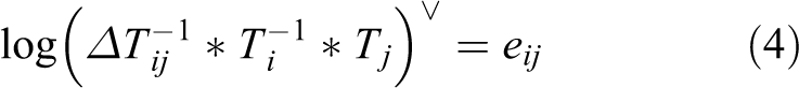
Notations: SO(3) denotes the special-orthogonal group which is a set of valid rotation matrices. SO(3) is corresponded with so(3) in Lie algebra. The homogeneous rigid transformation on robot poses can be described by the special Euclidean group SE(3). SE(3) is corresponded with se(3) in Lie algebra. “Log()” operator can transform SO(3)/SE(3) to so(3)/se(3). “∨” operator can transform so(3)/se(3) to SO(3)/SE(3).
The PGO problem is shown in Figure 1. We have measured relative transformation between node i and j, which corresponds to symbol Eij
in Figure 1. The target of PGO algorithm is to look for the best robot poses, which can make

Pose graph with odometry constraints with blue color and loop closure constraints with red color. Eij is the edge between pose i and pose j. The triangles represent the robot pose in world frame and the number in the triangles is the index of robot pose. There are two-loop closures in this graph, which are formed by robot poses {1,2,3,4} and {2,3,4,5,6,7,8}.
Initialization techniques
We know that PGO problem is a nonconvex problem, so the initial vales of estimated variable affect final iterative result. Good initial values advance iterative process to the global optimal solution. To obtain global optimal solution, a good initial state is an important step. For the time being, there are two strategies initializing PGO. The first one is COP-SLAM, 24 which uses analytical deduction to obtain initial pose of robot. The second one is based on two-step optimization. 25 The main idea is to solve for the rotations first and then estimate translation. We use experimental data to testify that the two-step algorithm is more accurate than COP-SLAM algorithm and the result is shown in the fifth section. We give brief descriptions about two-step algorithm below:
We use Lie algebra to form the first cost function

After initialization of rotation matrix, we form translation cost function as follows

Ri
has been known and
COP-SLAM produces analytical initial results, which are easily affected by noise data. But two-step initialization algorithm uses nonlinear optimization algorithm which can use M-estimator function to reduce effect of noise. So two-step initialization technique is more accurate than COP-SLAM algorithm and experimental results are shown in the fifth section. In our G-PGO algorithm, we use two-step algorithm to initialize PGO values.
PGO cost function
After initialization step, we have obtained initial values of robot pose. The next step is to form nonlinear cost function to polish initial result. Different types of cost function and the Jacobian matrix lead to different final results. There are three types of cost function, which have been given in previous articles. In this article, we compare their performances using real-world data and prove which is more accurate. Here we give three cost functions directly: Equation (3) is from CERES library.
14
q is the unit quaternion and q* is the conjugation of unit quaternion. eij
is the residual error. qi
is the unit quaternion of robot pose with index i. ti
is the translation of robot pose with index i. Residual errors of (4) are in se(3) space. This cost function is widely used in many SLAM algorithms such as ORB-SLAM
32
In (5), the first three residual errors are in so(3) space and the last three residual errors are in Euclidean space. This cost function is used in Nasiri et al.
17
and Bai et al.
18


In CERES library, (3) is used as PGO cost function, and the Jacobian matrix of this cost function is obtained by automatic derivatives using Jets operations. 14 In (oriented FAST and rotated BRIEF) ORB-SLAM, the author uses (general graph optimizatio) G2O::EdgeSim3 structure to execute PGO optimization. In G2O::EdgeSim3, (4) is used as PGO cost function and the Jacobin matrix is obtained by numerical derivatives. Numerical derivative consumes much more time than analytical Jacobian matrix and iterative steps are larger than analytical ones. We show this phenomenon in the fifth section. In GTSAM library and “Robot State Estimation” book, analytical Jacobian matrix of (4) is derived. GTSAM library uses right multiplication to update pose, but Robot State Estimation book uses left multiplication to update pose. In Nasiri et al. 17 andBai et al., 18 (5) is employed as cost function of PGO algorithm and supplementary materials of Bai et al. 18 give analytical Jacobian matrix deduction.
We should note that the estimated variables of (5) are so(3) and translation vector. Thus nonlinear situation only occurs in rotation matrix R. It is different from (3) and (4) whose estimated variables are se(3) or unit quaternion and translation vector. The benefit of (5) is low nonlinear degree and more accurate result will be obtained. We compare batch PGO algorithms between CERES, GTSAM, ORB-SLAM, and (5). The experimental results are shown in the fifth section, which proves that (5) has smaller optimization steps and more accurate results.
G-PGO
It is easy for us to use (5) as cost function and corresponded Jacobian matrix to complete batch PGO. But batch PGO costs much more time, which cannot be finished online especially facing with large-scale areas. We want to estimate robot poses by recursively including recent loop closure measurement. This is incremental PGO algorithm. Here, we give an easy example to describe the differences between incremental and batch PGO.
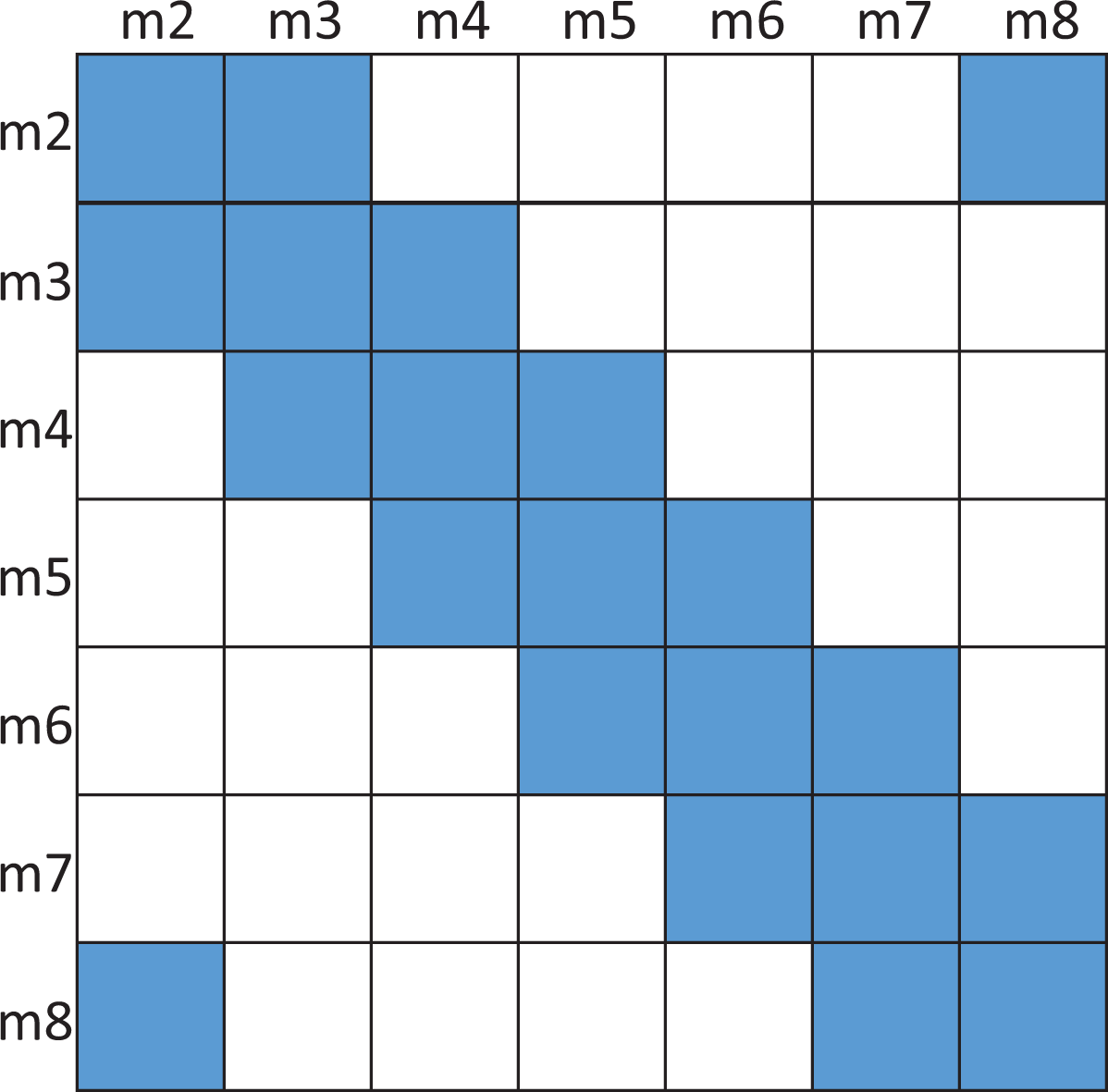
There are eight poses in Figure 1 in which two-loop closures exist. The first-loop closure is made up of robot poses {1,2,3,4} and the second-loop closure is made up of {2,3,4,5,6,7,8}. For simplicity, we only bring pose-chain constraints, which are constructed by the robot pose n and robot pose n + 1, into PGO. For off-line cases, we start batch PGO after obtaining robot pose 8. The Hessian matrix is shown in Figure 2. Off-line batch PGO optimizes all of robot poses at a time.

The Hessian matrix of batch PGO algorithm. The blue squares are filled by the Jacobian matrix and the white squares are empty. PGO: pose graph optimization.
In ORB and many other SLAM algorithms, they do not use Schur complement to marginalize variables, which are outside of slide windowing. They just optimize robot poses in the current loop closure. For example, in Figure 1, the robot moves to m4 position and the first PGO starts when the loop closure is detected. Then the Hessian matrix transforms to Figure 3. After the first PGO, we have got the optimized robot poses {1,2,3,4}. The second PGO starts when m2 and m8 construct a loop edge. The Hessian matrix of the second PGO is shown in Figure 4. This incremental PGO does not take m1 robot pose into consideration during the second PGO process.

The Hessian matrix of PGO algorithm when the first-loop closure is detected. The blue squares are filled by the Jacobian matrix and the white squares are empty. PGO: pose graph optimization.
The Hessian matrix of PGO algorithm when the second-loop closure is detected. The blue squares are filled by the Jacobian matrix and the white squares are empty. PGO: Pose graph optimization.
The incremental PGO should take FEJ problem into consideration. Compared with Figures 2 and 4, m1 is marginalized so the new Hessian matrix is

The Hessian matrix of correct incremental PGO algorithm when the second-loop closure is detected. The blue squares are filled by the Jacobian matrix and the white squares are empty. The red squares are affected by Schur complement and we should use the first-pose graph optimized pose results to calculate Jacobian matrices in red squares, which are related to robot pose m1. PGO: pose graph optimization
It is very complex to manage incremental algorithm because of consistency problem. The consistency problem can be solved by using initial Jacobian matrix, but it also leads to local optimal solution not the global optimal solution. We explain this situation in Figure 6. The estimated variables are x1 and x2. We have obtained initial values of x1 and x2 at point P1. P2 is the second iterative point if we optimize x1 and x2 together. P3 is the final global optimal solution. If we marginalize x1 at point P1, we obtain marginalized optimized result at P2′. The marginalized final solution is at P3′. At P1 point, we marginalize x1, so we do not update variable x1 in iterative step, and the iterative result comes to P2′ not P2. At P2′, we use direction which is obtained by P1 Jacobian to update x2. The third step’s iterative result is at P3′. The iterative process only can promise that the residual error decreases. If the residual error is larger than last step, the iterative process stops. We cannot promise that x2 of P3′ is equal to P3, so the marginalized result cannot converge to the global optimal solution. But if initial value P1 is close enough to P3, marginalized result P3′ is equal to P3.

The estimated variables are x1 and x2. Blue points are iterative results without marginalization and red points are iterative results with marginalization. We have obtained initial values of x1 and x2 at point P1. P2 is the second iterative point if we optimize x1 and x2 together. P3 is the final global optimal solution. If we marginalize x1 at point P1, we obtain marginalized optimized result at P2′. The marginalized final solution is at P3′.
Here, we put forward a new incremental PGO algorithm and simplify incremental PGO Hessian matrix management. We also take Figure 1 as an example to describe G-PGO. When the first loop is detected between m1 and m4, we execute batch PGO optimization which is described in (5). We obtain optimized robot poses {1,2,3,4}. We calculate poses between optimized robot poses, so relative poses
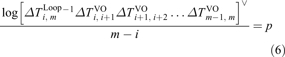
In (6),


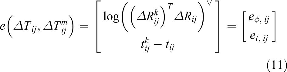
After removing wrong loop closure measurement, we construct the cost function for estimated variable

e is the cost function and Wk is the weight matrix which is the residual error produced by the kth loop closure optimization.
We design two different methods to form cost function
Method 1

Method 2
According to our experiments in lab, we find that these two methods produce the same result. The main reason is that every measurement is close to each other and these measurements are very close to global solution after deleting wrong edge information. So we just show one of results in the fifth section. Here, we describe the flow diagram of our G-PGO algorithm in Table 1.
The flow diagram of G-PGO algorithm.

PGO: pose graph optimization
Experimental results
In this section, we present experimental results of G-PGO algorithm. Section “Evaluation metrics” describes the performance metrics to evaluate PGO results. Section “Data sets” describes data sets we use in our experiments. Section “Results on data sets” evaluates the performance of PGO cost function in batch PGO and the comparison between G-PGO and ISAM.
Evaluation metrics
We use three data sets to verify our algorithm: KITTI, TUM, and New College data sets. KITTI and TUM data sets all provide six degree of freedom (6-dof) true poses, but true poses are not aligned in TUM data set, so we only can use python script from TUM data set to evaluate performances. This script outputs two indexes to describe accuracy: “AME” and “RME.” “AME” means absolute pose error, and “RME” means relative pose error. Specific definitions for “AME” and “RME” can be found in Sturm et al. 12
In KITTI data set, we use four metrics from Geiger et al. 11 for our evaluation. The first two metrics are absolute orientation and translation errors. These two errors are defined below


We also provide relative errors for evaluating errors. The relative errors are defined below


New College data set only provides true translation and the true pose is also not aligned. So the classic iterative closest point (ICP) algorithm is used to align optimized poses using half of data. The metric we use in New College data set is absolute translation error. Specific definitions for this error can be found in Smith et al. 13
Data sets
This article focuses on 3-D PGO algorithm. We search for PGO-related articles as many as possible. We find that most of articles only provide two-dimensional PGO data sets such as vertigo, 34 realizing, reversing and recovering (RRR), 23 G2O, 30 and switchable constraints. 35 Only COP-SLAM 8 provides 3-D PGO data sets, which include true poses by GPS and IMU. We use KITTI and New College data sets from COP-SLAM library in our experiments. The robot poses of VO in COP-SLAM data sets are obtained by LIBVISO2 36 and the loop closure detection is done by RTAB-MAP. 37 We also use TUM data set to evaluate batch PGO algorithm. We run ORB-SLAM algorithm on TUM data set. We forbid loop closure correction step in ORB-SLAM code but allow it to output loop closure information.
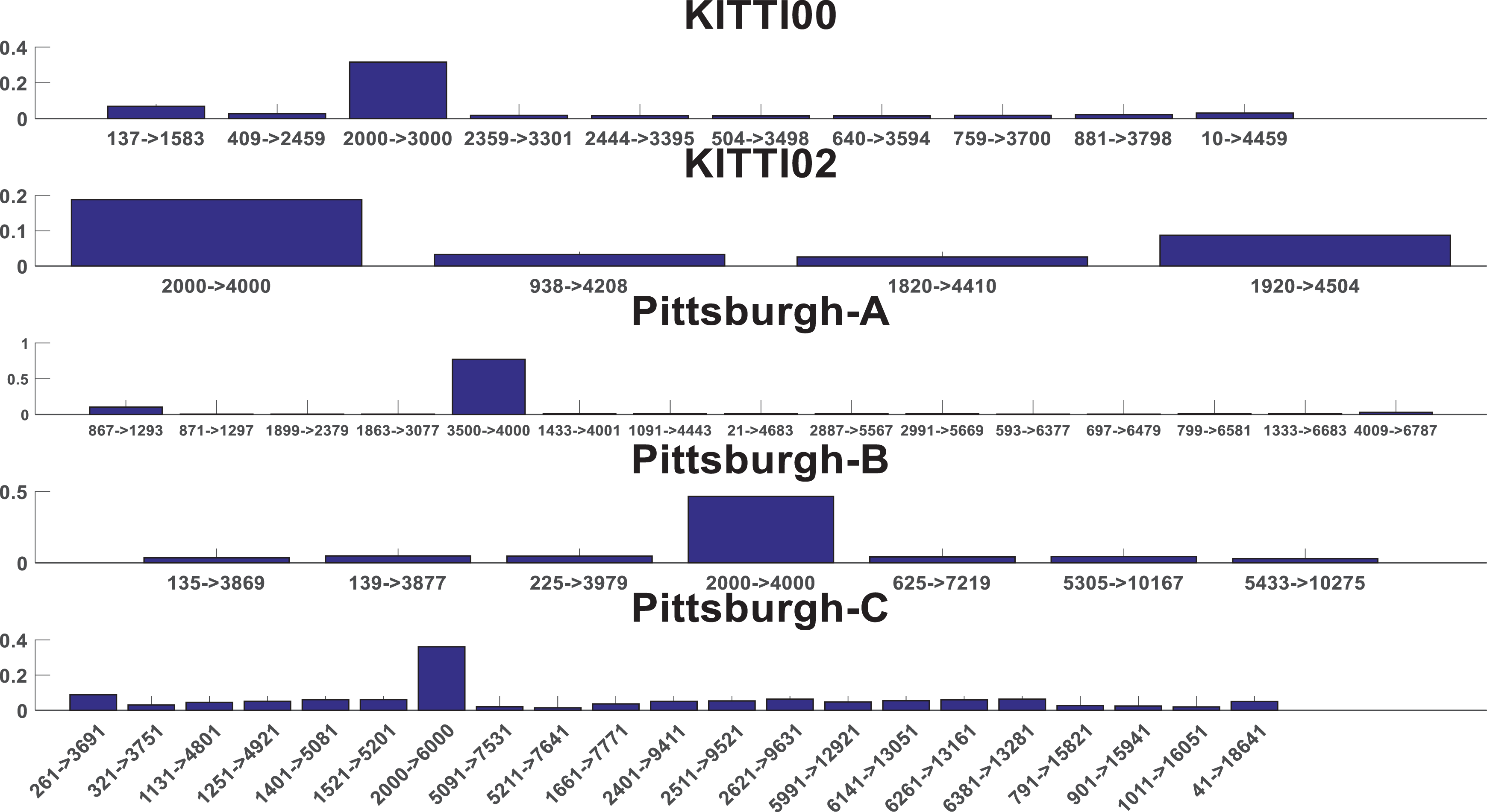
We use New College and KITTI data sets to evaluate PGO initialization algorithm, which is mentioned in “Initialization techniques” section. We use TUM and KITTI data sets to evaluate batch PGO algorithm, which is mentioned in “PGO cost function” section. We use New College and TUM data sets to evaluate incremental PGO algorithm, which is which is shown in Figure 7. The true and VO poses of these data sets are plotted in Figure 7. The first figure in Figure 7 is the robot pose. Red color trajectory is the true trajectory and blue color is the trajectory of odometry. The second figure in Figure 7 is loop closure information in every data set. The x-axis is the index of robot pose and the y-axis is the start index and end index in every loop.

The figures in left column are plotted by true robot poses and VO robot poses. The unit is meter. The figures in right column are plotted by loop closure information. The x-axis is the robot pose index and the y-axis is the range of robot pose which is included in the loop closure. VO: visual odometry.

KITTI00 sequence is shown in (a) whose total length is 4 km. KITTI02 sequence is shown in (b) whose total length is 5 km. New College Pittsburgh-A data set is shown in (c) whose total length is 8 km. New College Pittsburgh-B data set is shown in (d) whose total length is 14 km. New College Pittsburgh-C data set is shown in (e) whose total length is 19 km. Figure (f) from the first to the last are TUM-freiburg1_room data set, TUM-freiburg2_desk data set, and freiburg3_long_office data set. Because there is only one loop closure in TUM data set, so TUM data set is not used to evaluate incremental PGO algorithm. Total length of Figure (f) from the first to the last is 17.4834 m, 20.34 m, and 22.2 m.
Results on data sets
First, we give the performance of initial algorithm for PGO. Second, we compare our batch PGO algorithm. Finally, we prove that G-PGO is accurate and robust in solving incremental PGO problem.
Initialization results
Initialization step is to guarantee that initial state of nonlinear optimization is close to global optimal solution. We compare initialization results between COP-SLAM and two-step initialization method. Here, we use KITTI and TUM data sets to evaluate initialization algorithm. New College data set cannot provide 6-dof true poses, so we do not use it here. Pittsburgh data sets provide 6-dof true pose, but VO poses and true poses are not in the same coordinate. So we just use absolute pose error to evaluate performances. We can see from Tabel 2 that absolute translation, absolute rotation, and relative rotation errors decrease after initialization algorithm. “Na” in Table 2 is the meaning of none value which represents data sets do not provide true value or optimization failure. Data set Pittsburgh_A, Pittsburgh_B, and Pittsburgh_C only provide true absolute translation values, so the values in 3 columns are “Na.” It can be seen from Table 2 that two-step initialization method leads to smaller absolute translation, absolute rotation, and relative translation errors compared with COP-SLAM algorithm. It proves that two-step initialization algorithm is more accurate than COP-SLAM algorithm. But one thing to note is that relative translation error becomes larger after initialization algorithm, which is marked red in Table 2. The main reason is that two-step algorithm divides the optimization process into two steps. The first step is to optimize rotation matrix and fix the translation. The second step is to optimize translation but fix rotation matrix. The optimized variables of initialization technique are absolute poses in the world frame, so nonlinear optimization adjusts the absolute variables to close loops but the direction of adjustment is to decrease corresponded cost function not the whole cost function like batch PGO. We can see from (2) that rotation matrix affects translation error, and two-step optimized algorithm does not optimize rotation matrix and translation together. It is the drawback of initialization step and we use batch PGO algorithm to polish initialization results in the next step.
The initialization technique result compared between COP-SLAM and two-step method. KITT00, KITTI02, Pittsburgh_A, Pittsburgh_B, and Pittsburgh_C data sets are used to evaluate performances. Four metrics in columns are corresponded with (12)–(16).

COP: closed-form PGO; SLAM: simultaneous localization and mapping; VO: visual odometry; PGO: pose graph optimization
Batch PGO results
After initialization process, we use batch PGO to optimize all of robot poses in world frame. The batch PGO algorithm is suitable for off-line situation. Here, we use KITTI00, KITTI02, and TUM data sets to compare different cost functions. Table 3 displays results of KITTI data sets and Table 4 displays results of TUM data sets. Values in steps column mean that how many steps are needed to finish optimization. “Na” in steps column represents optimization failure.
The batch optimization performances between CERES, ORB, Robot State Estimation, and our method using KITTI data set. We set the max iteration step 50 and if the iteration step is larger than 50, the iteration will stop and output results.
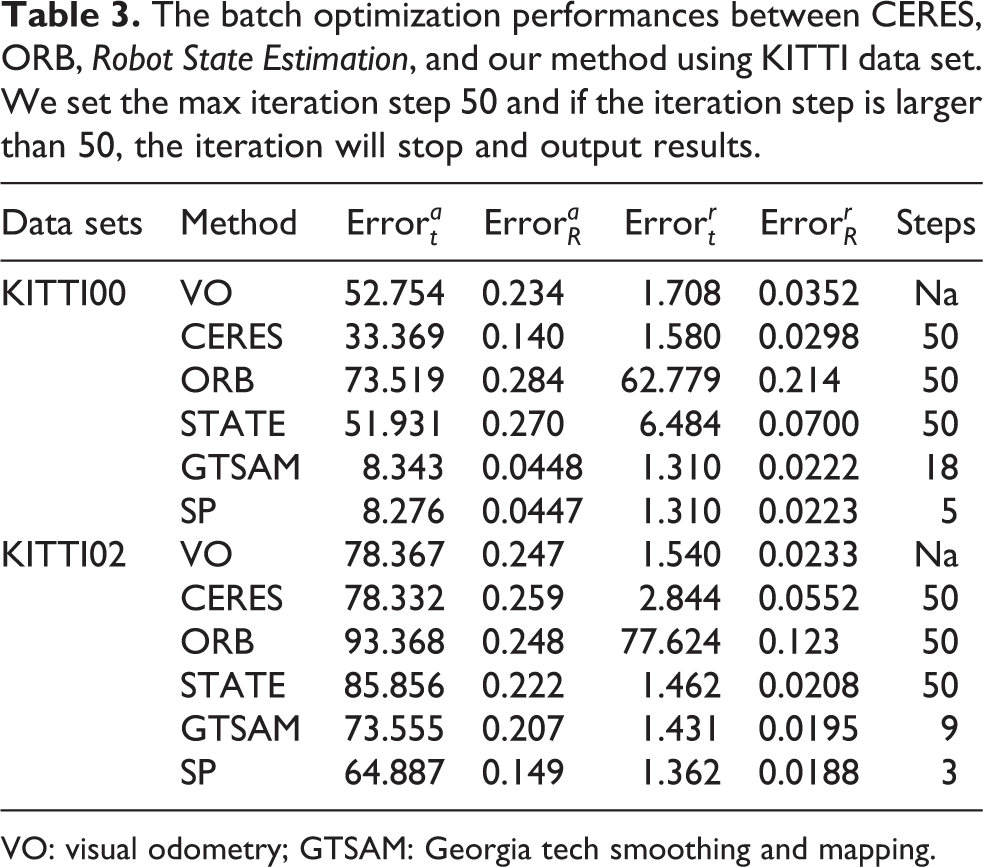
VO: visual odometry; GTSAM: Georgia tech smoothing and mapping.
The batch optimization performances between CERES, ORB, Robot State Estimation, and Our method using TUM sequence data set. We set the max iteration step 50 and if the iteration step is larger than 50, the iteration will stop and output results.
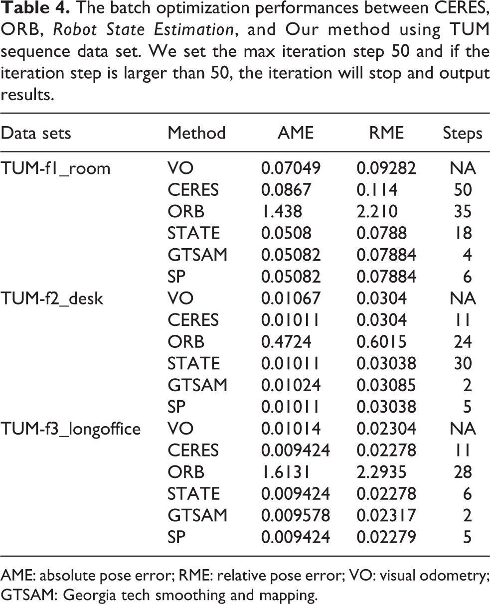
AME: absolute pose error; RME: relative pose error; VO: visual odometry; GTSAM: Georgia tech smoothing and mapping.
CERES in Tables 3 and 4 is corresponded with cost function (3). ORB is corresponded with cost function (4) and the Jacobian matrix is obtained by numerical method. STATE is corresponded with cost function (4) and the Jacobian matrix is obtained by left multiplication analytical deduction. GTSAM is corresponded with cost function (4) and the Jacobian matrix is obtained by right multiplication analytical deduction. Separated process (SP) is corresponded with cost function (5) and the Jacobian matrix is obtained by analytical deduction.
After batch optimization, relative translation error is smaller than odometry, and robot pose is closer to true solution. That is the reason why we need batch optimization after initialization process. We can see from Tables 3 and 4 that the convergence speed of CERES and ORB is very slow. The worst problem of CERES method is that it does not direct the optimization process to the global optimal solution which can be seen from KITTI02 and TUM-f1_room. The main reason of ORB’s bad performance is that ORB uses numerical Jacobian matrix to update poses in iterative process. We have talked about numerical Jacobian matrix before, and it is much less accurate than analytical Jacobian matrix. Another problem is that CERES uses automatic derivation; it costs more iterative steps than analytical Jacobian matrix. We can see from KITTI00, KITTI02, and TUM-f1 that CERES needs more than 50 steps to finish optimization which means that its time cost is very large. But we have to say that ORB SLAM code is not totally wrong. In ORB SLAM source code, the PGO algorithm deals with only one loop but our batch experiment includes more than loop closures. The PGO algorithm of ORB-SLAM source code performs not bad facing only one loop closure. Robot State Estimation (STATE), GTSAM, and SP PGO algorithms perform much better than CERES and ORB. The main reason is that these three algorithms use analytical Jacobian matrix and Lie algebra as cost function.
We can see from KITTI00, KITTI02, TUM-f2, and TUM-f3 data sets that SP algorithm is more accurate than CERES, ORB, and STATE algorithms. Another important superiority is that SP has the smallest optimized steps because of its cost function’s lower nonlinearity. Although steps of GTSAM in TUM-f3 and TUM-f2 are smaller than SP, SP algorithm is more accurate. According to our experiments, we choose SP model to optimize batch PGO in our G-GPO algorithm. The accuracy of final result is also dependent on the way you solve linear equation. We have to admit that different open source library such as G2O, GTSAM, and CERES uses different strategies to solve linear equation. But in our experiment, we just compare different cost function and open source library and choose the best performance one which is used in our G-PGO algorithm
Incremental PGO results
The last experiment is incremental experiment. We use KITTI00, KITTI02, and New College data sets to verify G-PGO algorithm. TUM data set only contains one-loop closure, so we do not use it here. True poses are aligned in KITTI data set, but true poses are not aligned in New College data set. When dealing with New College data set, we use half of true poses and optimized poses to align two coordinates. Classic ICP algorithm 38 is used here to align two coordinates. After aligning two coordinates, we use absolute translation error, which is described in the fifth section, to evaluate incremental PGO algorithms. In Table 5, we divide experimental results into two classes. The first class is noise free data which means that wrong loop closure information is not added into input data. Results of noise free data is listed in the second and third row of Table 5. Another class is noisy input data. We add wrong loop closure information in data, and wrong loop closure information in every data set is shown in red color in Figure 9. The last two rows in Table 5 are results of noisy data.
The experimental results of incremental PGO algorithm. Sequential PGO method is the Schur way of ORB-SLAM source code executing PGO. The unit of every element in table is meter.
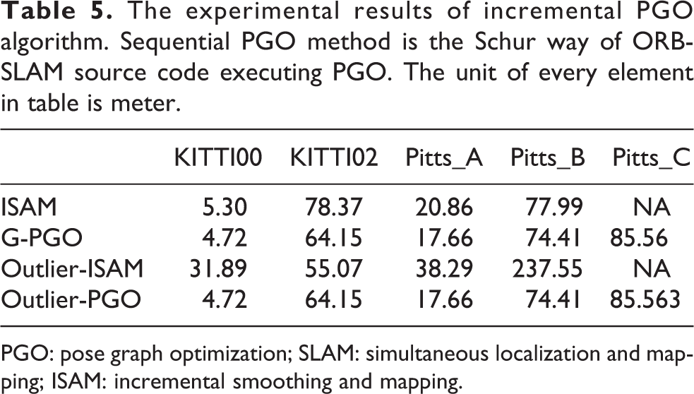
PGO: pose graph optimization; SLAM: simultaneous localization and mapping; ISAM: incremental smoothing and mapping.
We can see from Table 5 that our algorithm performs better than ISAM algorithm no matter in noise free data or noisy data. Our algorithm has smaller absolute trajectory error (ATE) in these five data sets. Especially in Pittsburgh_C data set, ISAM fails to optimize robot poses and our algorithm outputs accurate result. The main reason is that ISAM uses Orthogonal Triangle (QR) factorization process to reduce the amount of calculation and FEJ algorithm is used to promise consistency during optimization. But as we discuss in fourth section, this algorithm cannot promise to converge to global best solution. Our algorithm makes full use of every loop closure’s information and produces more accurate results. The optimized robot trajectories produced by G-PGO are shown in Figure 8.

The red trajectory is true robot pose and the blue trajectory is G-PGO result. KITTI00 sequence is shown in (a) and KITTI02 sequence is shown in (b). Pittsburgh_A sequence from New College data set is shown in (c). Pittsburgh_B sequence from New College data set is shown in (d). Pittsburgh_C sequence from New College data set is shown in (e). PGO: pose graph optimization.
We can see from Table 5 that G-PGO performs better than classic incremental PGO algorithm especially in the outlier free case. ISAM algorithm directs iterative process to wrong direction and ATE becomes even larger after optimization compared with odometry result. G-PGO uses constraint metric to exclude wrong loop closure information and produces the same result with noise free data. In Figure 9, we display wrong loop closure information. The Y-axis of Figure 9 is constraint metric which is corresponded with (6). The X-axis of Figure 9 is corresponded with loop closure in every data set. The label of X-axis is robot pose index, which leads to a loop closure. Red bar is wrong loop closure information we add. We can see from Figure 9 that constraint metric of wrong loop closure is much larger than correct ones. So wrong loop closure can be easily deleted from input data.
Outlier metric is shown in this figure. We add wrong loop closure information in edges, which is represented by red bar.
Conclusions
In this article, we review the previous PGO algorithms that include initialization algorithm and cost function. We compare two-step initialization algorithm and COP-SLAM in large real scenes. We find that two-step initialization algorithm performs better than COP-SLAM. Two-step algorithm estimates the rotation matrix without taking translation into consideration and thenes fix the optimized rotation matrix to solve linear equation to obtain translation of robot pose. This step guarantees that the initial robot poses are not far from the global optimal solution. After initialization process, we compare different cost functions used in PGO. We find that SP model is more accurate than others. In this model, the estimated variables are so(3) and translation. The benefit of this cost function is to decrease the nonlinearity of cost function compared with others. At last, to bypass the Schur complement and consistency problem of incremental PGO, we put forward a new incremental PGO algorithm named G-PGO. G-PGO does not optimize the absolute robot pose in the world but the estimated variables are relative robot poses. Every loop closure performance is introduced into the G-PGO cost function as weight matrix to balance measured relative poses. Another superiority is that G-GPO algorithm can delete wrong loop closure information using constraint metric automatically. We compare G-PGO with ISAM algorithm. G-PGO performs much better than ISAM result and G-PGO is also more robust to outliers than ISAM. In our future work, we will focus on observability of PGO algorithm and to testify what kind of loop closure can obtain accurate results according to their observability.
Footnotes
Declaration of conflicting interests
The author(s) declared no potential conflicts of interest with respect to the research, authorship, and/or publication of this article.
Funding
The author(s) disclosed receipt of the following financial support for the research, authorship, and/or publication of this article: This work was supported by the national natural science foundation of china (Grant ID-61601123), national basic research program of china (973 program) (Grant ID-2016YFB0502103) and natural science foundation of jiangsu province (Grant ID-BK20160696).