Network- and CFD/CAA-modelling of the high frequency flame response in multi-jet combustors

Abstract

Low order networks are widely used for linear stability analysis of combustors in the low frequency limit. High frequency stability analysis, however, is limited to cost-intensive numerical or experimental methods, since derivation of analytical solutions is either cumbersome or impossible. The article at hand provides a quasi-two-port network model for the effective modal acoustic pressure and axial velocity normalised with the transverse acoustic field for cylindrical combustors. This network modelling approach includes transfer matrices of acoustic area jumps, ducts for longitudinal, standing and spinning transverse and mixed mode wave propagation. The purely acoustic transfer matrices are validated with a generic non-reactive experiment. On the basis of phase-locked $\mathrm{OH}*$ images of an engine-similar multi-jet combustor with a forced T1 mode, a locally distributed flame response model is derived, which is reduced to a global flame transfer matrix. A locally resolved convective flame response model is implemented in a numerical model in order to verify the provided theory by the comparison of the analytical and numerical flame transfer matrix for the high-frequency regime.

Introduction

Although high-frequency thermoacoustic instabilities are a known, particularly damaging threat for rocket and gas turbine engines, a lack of fundamental, analytical understanding of the thermoacoustic coupling conditions and low-cost linear stability analysis tools for industrial application is present. The existing concepts from the low-frequency (LF) regime provide the theoretical base for the present work and are, therefore, summarised briefly. In an early design stage, linear combustor stability analyses of longitudinal combustion instabilities are carried out analytically employing low-order network models assuming an infinitely thin flame^3,2,1 or numerically using the state-of-the-art hybrid computational fluid dynamics/computational aeroacoustics (CFD/CAA) approach and a locally resolved flame response,^5,4,6 both avoiding expensive unsteady computational fluid dynamics (CFD) simulations. Considering perfectly premixed combustors, acoustic velocity fluctuations at the burner mouth are considered as the dominant cause of injector-coupled LF combustion instabilities in gas turbines. More recently, increasing evidence is provided for the significant contribution of acoustic velocity fluctuations in the high-frequency (HF) regime.^8,7,9,10 Concerning analytical network tools, distributed time delay models ¹¹ using the assumption of a compact flame at one axial position in the domain to couple the integral heat release fluctuations to the axial acoustic velocity fluctuations at the reference position by means of an integral flame transfer function (FTF) are state-of-the-art. The acoustic pressure $p_b^{\prime }=p_u^{\prime }$ and the acoustic velocity $u_b^{\prime }{A}_b=u_u^{\prime }{A}_u+\frac{\kappa -1}{\kappa \overline{p}}{\dot{Q}}^{\prime }(t-\tau )$ jump conditions across a flame are the core of every thermoacoustic low-order model, coupling the unburned and burned gas state of the acoustic system.^12,13 In this context, the goal of the article at hand is to preserve the most dominant physical effects in a simplified network model to predict and understand the complex HF thermoacoustic coupling mechanisms, providing an extension of the analytical concepts from LF thermoacoustics to the HF regime. Can annular combustors with longitudinal wave propagation inside the cans and the annulus provide first numerical and analytical insights on transverse to longitudinal acoustic coupling^{12,17,15,16,14} as well as the flame response by means of an infinitely thin flame at the exit of the cans.^20,19,18 Modelling of HF can combustors is mainly limited to numerical models. Analytical models are the exception, due to the complex three-dimensional acoustic mode structure. To the knowledge of the authors Dowling et al. ²¹ were the first to investigate HF stability analysis for cylindrical gas turbine combustors analytically including a time-delay model in the injector tubes. Besides the convective source, the highly non-compact flame response due to flame displacement and compression^23,22 might play a role for HF thermoacoustic stability analysis. The numerical linear hybrid CFD/CAA stability analysis tools are extended by Hummel et al. ²⁴ accounting for local flame displacement and compression and validated with results of Berger et al. ²⁵ In the present work, the hybrid CFD/CAA tools are extended by a simple, locally resolved convective flame response model for the specific case of a multi-jet combustor (MJC). The main focus of the article, however, lies on the novel HF quasi-two-port network modelling approach, based on Rosenkranz et al., ²⁶ to overcome the limitation to numerical models and to improve the understanding of the basic mechanisms causing HF combustion instabilities.

Inhomogeneous wave equation

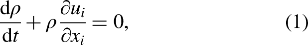
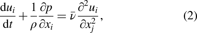
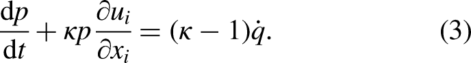
The following derivation of the thermoacoustic models starts from the inhomogeneous wave equation obtained from the conservation of mass, momentum and energy. In the present work, the compressible mass, momentum and energy conservation are expressed in terms of the acoustic field variables, that is, pressure and velocity according to Dowling et al.,^21,1 assuming heat release of an unburned, ideal gas mixture as the only dominant source in the energy conservation

$$\frac{\mathrm{d}\rho }{\mathrm{d}t}+\rho \frac{\mathrm{\partial }{u}_i}{\mathrm{\partial }{x}_i}=0$$

(1)

$$\frac{\mathrm{d}{u}_i}{\mathrm{d}t}+\frac{1}{\rho }\frac{\mathrm{\partial }p}{\mathrm{\partial }{x}_i}=\overline{\nu }\frac{{\mathrm{\partial }}^2{u}_i}{\mathrm{\partial }{x}_j^2}$$

(2)

$$\frac{\mathrm{d}p}{\mathrm{d}t}+\kappa p\frac{\mathrm{\partial }{u}_i}{\mathrm{\partial }{x}_i}=(\kappa -1)\dot{q}$$

(3)

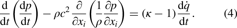
The material derivative of the energy conservation $\frac{\mathrm{d}}{\mathrm{d}t}$ and the gradient $\frac{\mathrm{\partial }}{\mathrm{\partial }{x}_i}=\mathrm{\nabla }$ of the momentum conservation multiplied by $\rho c^2=\kappa p$ yields the non-linearised formulation of the inhomogeneous convective wave equation. In the classical form of the convective wave equation, a homogeneous mean flow and thus no gradients in velocity are required. Note that the gradients in velocity can also be accounted for by the choice of proper boundary conditions as shown by Heilmann et al. ²⁷ and are, therefore, omitted in the following, which yields

$$\frac{\mathrm{d}}{\mathrm{d}t}\left(\frac{\mathrm{d}p}{\mathrm{d}t}\right)-\rho c^2\frac{\mathrm{\partial }}{\mathrm{\partial }{x}_i}\left(\frac{1}{\rho }\frac{\mathrm{\partial }p}{\mathrm{\partial }{x}_i}\right)=(\kappa -1)\frac{\mathrm{d}\dot{q}}{\mathrm{d}t}$$

(4)

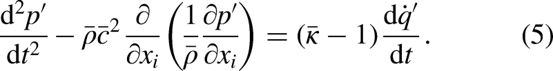
Linearisation around the time averaged mean value for all variables ${\phi }^{\mathrm{\prime }}=\phi (t,\mathbf{x})-\overline{\phi }(\mathbf{x})$ yields the inhomogeneous wave equation

$$\frac{{\mathrm{d}}^2{p}^{\prime }}{\mathrm{d}{t}^2}-\overline{\rho }{\overline{c}}^2\frac{\mathrm{\partial }}{\mathrm{\partial }{x}_i}\left(\frac{1}{\overline{\rho }}\frac{\mathrm{\partial }{p}^{\prime }}{\mathrm{\partial }{x}_i}\right)=(\overline{\kappa }-1)\frac{\mathrm{d}{\dot{q}}^{\prime }}{\mathrm{d}t}$$

(5)

The linearisation of the source term with respect to solely acoustic fluctuations reads

$$\frac{\mathrm{d}{\dot{q}}^{\prime }}{\mathrm{d}t}=\frac{\mathrm{\partial }{\dot{q}}^{\prime }}{\mathrm{\partial }t}+{\overline{u}}_j\frac{\mathrm{\partial }{\dot{q}}^{\prime }}{\mathrm{\partial }{x}_j}+u_j^{\prime }\frac{\mathrm{\partial }\overline{\dot{q}}}{\mathrm{\partial }{x}_j}$$

(6)

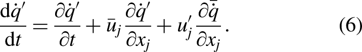
The linearisation of the material derivative (equation (6)) consists of the local unsteady change and the convective transport of the heat release rate fluctuations as well as the displacement of the mean heat release field. The low Mach number assumption yields the neglection of convective effects in the wave equation including the neglection of the mean flow in equation (6). A heat release density closure model is required to couple the acoustic pressure and velocity to the flame response, as discussed in the next section.

Flame response model

This section aims to extend the premixed HF thermoacoustic coupling models, that is, flame compression and displacement by the convective source terms with regard to the application to fully three-dimensional reduced and low-order combustor models.

In order to evaluate the local flame response, a closure model for the heat release rate density is required. Considering finite rate chemistry, the local heat release rate density is equal to the sum of formation enthalpies due to the chemical reaction $\dot{q}=-{\mathrm{\Sigma }}_r{\dot{\omega }}_r{\mathrm{\Delta }}_R{h}_r$ , where the reaction rate might be given by the change of molar fuel concentration $c_F$ in time. Premixed combustion models reduce the complex finite rate chemistry to a single non-dimensional reaction progress variable $C_r$ which yields ${\dot{\omega }}_r=\frac{\mathrm{d}{C}_r}{\mathrm{d}t}{c}_F=\frac{\mathrm{d}{C}_r}{\mathrm{d}t}\frac{\rho }{M_F}{Y}_F$ . Therefore, the heat release rate density is given by

$$\dot{q}=\rho \dot{\mathrm{\Omega }}{Y}_F{H}_F$$

(7)

the density $\rho$ , the normalised reaction rate $\dot{\mathrm{\Omega }}=\frac{\mathrm{d}{C}_r}{\mathrm{d}t}$ , the fuel mass fraction $Y_F$ and the lower caloric heating value $H_F$ . The linearised heat release rate density according to equation (7) yields

$${\dot{q}}^{\prime }={\rho }^{\prime }{\overline{\dot{\mathrm{\Omega }}}}_r\overline{Y_F}\overline{H_F}+\overline{\rho }{\dot{\mathrm{\Omega }}}_r^{\prime }\overline{Y_F}\overline{H_F}$$

(8)

where fluctuations in the fuel mass fraction, entropy waves and the lower caloric heating value are neglected considering perfectly premixed combustion.

Acoustic flame response

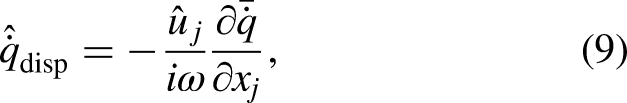
The flame response due to the local acoustic fluctuations in pressure and velolcity is referred to as acoustic flame response, which covers the flame compression and displacement mechanism. The material derivative of the inhomogeneous source term in the wave equation is linearised with respect to the acoustic fluctuations. Thus, the flame displacement mechanism in frequency domain reads

$${\hat{\dot{q}}}_{\mathrm{disp}}=-\frac{{\hat{u}}_j}{i\omega }\frac{\mathrm{\partial }\overline{\dot{q}}}{\mathrm{\partial }{x}_j}$$

(9)

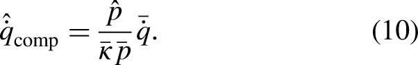
according to the last term in equation (6), where the linearised momentum conservation assuming a low Mach number might be used to obtain the local velocity fluctuations ${\hat{u}}_j=-\frac{1}{i\omega \overline{\rho }}\frac{\mathrm{\partial }\hat{p}}{\mathrm{\partial }{x}_j}$ . The isentropic, acoustic density fluctuations in equation (8) are accounted by the flame compression mechanism which reads

$${\hat{\dot{q}}}_{\mathrm{comp}}=\frac{\hat{p}}{\overline{\kappa }\overline{p}}\overline{\dot{q}}$$

(10)

The acoustic flame displacement and compression mechanisms are established flame response models depending on the local acoustic and mean heat release rate field.^24,23 The convective driving mechanism, however, requires an additional transport model to couple the local acoustic pressure and velocity to the convective source, as discussed in the following section.

Convective flame response

The irrotational, acoustic velocity fluctuations at the injector tube exit, that is, the reference position periodically modulate the Kelvin Helmholtz instability in the shear layer resulting in coherent vortex structures. These coherent vortex structures lead to a local fluctuation in the normalised reaction rate, which concerning premixed combustion, might be obtained via the level set method.^28,30,29 Neglecting curvature and diffusive effects the displacement speed of the flame front is equal to the turbulent flame speed, which yields the propagation of the flame surface $C_r=const$ according to

$$\dot{\mathrm{\Omega }}=\frac{\mathrm{\partial }{C}_r}{\mathrm{\partial }t}+u_j\frac{\mathrm{\partial }{C}_r}{\mathrm{\partial }{x}_j}=s_t\left|\frac{\mathrm{\partial }{C}_r}{\mathrm{\partial }{x}_j}\right|$$

(11)

For quasi-steady combustion ( $\frac{\mathrm{\partial }{C}_r}{\mathrm{\partial }t}=0$ ), equation (11) simplifies to the kinematic balance of the flame front normal component of the local velocity vector $u_n=-u_j{n}_{\mathrm{Fl},j}$ and the turbulent flame speed $s_t$

$$-u_j{n}_{\mathrm{Fl},j}=s_t$$

(12)

with the local flame surface normal vector $n_{\mathrm{Fl},j}$ pointing in unburned gas direction $n_{\mathrm{Fl},j}=-\frac{\mathrm{\partial }{C}_r}{\mathrm{\partial }{x}_j}/\sqrt{(\frac{\mathrm{\partial }{C}_r}{\mathrm{\partial }{x}_j}{)}^2}$ as sketched in Figure 1. The normalised consumption rate (equation (11)) simplifies to

$$\dot{\mathrm{\Omega }}=-u_j{n}_{\mathrm{Fl},j}{\sigma }_{\mathrm{Fl}}$$

(13)

Here the flame surface density ${\sigma }_{\mathrm{Fl}}=\sqrt{(\frac{\mathrm{\partial }{C}_r}{\mathrm{\partial }{x}_j}{)}^2}$ is introduced corresponding to the spatial probability density function of the flame front, ²⁹ which is constant concerning a quasi-steady response model. The common quasi-steady assumption $n_{\mathrm{Fl},j}{\sigma }_{\mathrm{Fl}}=const$ in low-order models^1,3,31 is in line with the hybrid CFD/CAA approach, which couples the mean flow solely to the acoustic model, avoiding additional transport equations for the flame surface density. According to equation (13), the coherent vortex structures modulating the flame front normal velocity $u_n$ , might originate from irrotational acoustic velocity fluctuations in all directions in space $u_j{n}_{\mathrm{Fl},j}=u_x{n}_{\mathrm{Fl},x}+u_r{n}_{\mathrm{Fl},r}+u_{\phi }{n}_{\mathrm{Fl},\phi }$ at the reference position. Concerning the investigated case of a injector coupled MJC, however, the axial acoustic velocity of the unburned gas at the reference position, see Figure 1, is the predominant cause of the flame front normal velocity fluctuations ¹⁰ as also observed in can annular combustors.^8,20 The linearisation of equation (13) for the quasi-steady flame front yields

$$\dot{\mathrm{\Omega }}={\hat{u}}_{n,v}{\sigma }_{\mathrm{Fl}}$$

(14)

accounting for the front normal velocity fluctuations of the coherent vortices ${\hat{u}}_{n,v}$ . A hydrodynamic transport model for the coherent turbulent velocity fluctuations ${\hat{u}}_v$ is obtained from the linearised momentum conservation equation (2) in frequency domain

$$i\omega {\hat{u}}_v+\overline{u}\frac{\mathrm{\partial }{\hat{u}}_v}{\mathrm{\partial }x}+\frac{1}{\overline{\rho }}\frac{\mathrm{\partial }\hat{p}}{\mathrm{\partial }x}=\overline{\nu }\frac{{\mathrm{\partial }}^2{\hat{u}}_v}{\mathrm{\partial }{x}_j^2}$$

(15)

The axial gradient in acoustic pressure is negligible in comparison to the convective transport of the coherent velocity fluctuations in unburned gas mixture $\frac{1}{\overline{\rho }}\frac{\mathrm{\partial }\hat{p}}{\mathrm{\partial }x}\ll \overline{u}\frac{\mathrm{\partial }{\hat{u}}_v}{\mathrm{\partial }{x}_j}$ . According to turbulent jet theory ³² the length scale of the coherent vortices increases with axial distance from the reference position during the convective transport, due to the entrainment of surrounding exhaust gas associated with a decrease in convection velocity. The volume expansion due to combustion might compensate the decrease in axial convection speed, which reasons the assumption of a net constant convection velocity. The coherent vortices eventually dissipate for a large distance from the reference position $x/d_T\gg 10$ . Thus, dissipative effects become a significant impact factor especially for higher turbulence levels, i.e., lower turbulent Reynolds numbers. Therefore, a convective-diffusive model accounting for turbulent/molecular dissipation is provided in the Appendix, which accounts for the decreasing amplitude of the coherent velocity fluctuations along the stream line from the reference position to the flame. However, premixed jet flames predominantly exist close to the unburned gas jet core region $x/d_T<10$ . Thus, the dissipation of the coherent vortices with axial distance becomes negligible for high turbulent/molecular Reynolds numbers. ³³ Note that experimental results by Rosenkranz et al. ¹⁰ as well as the results provided below support these hypotheses.

Figure 1.

Sketch of an axial cut through a cylindrical multi-jet combustor (MJC) with combustion chamber diameter $d_C$ at the centre of a single injector tube with diameter $d_T$ and a jet flame represented by the reaction progress variable iso-contour $C_r=0.5$ with deflagrative flame stabilisation at the kinematic balance of the turbulent flame speed $s_t$ and the flame normal velocity of unburned gas $u_n$ close to the core region of the turbulent jet.

Thus, a simplified transport model for negligible dissipation and spatially constant mean flow velocity is obtained by integration from the reference position $x_{\mathrm{ref}}$ to the local flame position

$${\hat{u}}_v(x)={\hat{u}}_v(x_{\mathrm{ref}})e^{-i{k}_{\mathrm{conv}}(x-x_{\mathrm{ref}})}$$

(16)

which yields the constant convective wave number $k_{\mathrm{conv}}=\frac{\omega }{\overline{u}}$ . Although the mean velocity $\overline{u}$ might be constant over the extent of the flame, it might deviate to lower values compared to the theoretical injector tube velocity, since the flame requires a certain degree of mixing with the recirculated exhaust gas to ignite. Considering a simple mixing law $\overline{u}=Y_u{\overline{u}}_u+Y_b{\overline{u}}_b$ . Assuming negligible surrounding burned gas velocity ${\overline{u}}_u\gg {\overline{u}}_b$ yields the unburned gas mixture fraction at the flame front $Y_u={\dot{m}}_u/({\dot{m}}_u+{\dot{m}}_b)$ as correction parameter

$$\overline{u}=Y_u{\overline{u}}_u$$

(17)

of the coherent vortex convection speed. The values of $Y_u$ are expected to be close to unity for a flame stabilisation close to the unburned jet core region.

The closure of the heat release rate density to the local coherent velocity fluctuation is given by the combination of the quasi-steady level-set-method (equation (13)) with the normalised heat release rate density fluctuations according to equation (8) which yields

$$\frac{\hat{\dot{q}}}{\overline{\dot{q}}}=\frac{{\widehat{\dot{\mathrm{\Omega }}}}_r}{{\overline{\dot{\mathrm{\Omega }}}}_r}=\frac{{\hat{u}}_v}{\overline{u}}$$

(18)

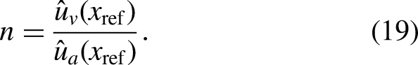
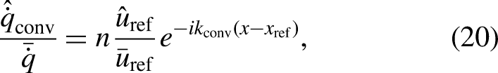
The coupling of the coherent turbulent fluctuations ${\hat{u}}_v$ to the acoustic velocity fluctuations ${\hat{u}}_a$ at the reference position is obtained via a prescribed hydrodynamic gain

$$n=\frac{{\hat{u}}_v(x_{\mathrm{ref}})}{{\hat{u}}_a(x_{\mathrm{ref}})}$$

(19)

Finally, the combination of equations (19) and (18) yields the convective contribution of the flame response due to axial acoustic velocity fluctuations at the reference position

$$\frac{{\hat{\dot{q}}}_{\mathrm{conv}}}{\overline{\dot{q}}}=n\frac{{\hat{u}}_{\mathrm{ref}}}{{\overline{u}}_{\mathrm{ref}}}{e}^{-i{k}_{\mathrm{conv}}(x-x_{\mathrm{ref}})}$$

(20)

which is an analogous spatially resolved formulation of the $n$ - $\tau$ -modelling approach in LF thermoacoustics with the restriction to the axial mean flow direction.

Hybrid CFD/CAA model

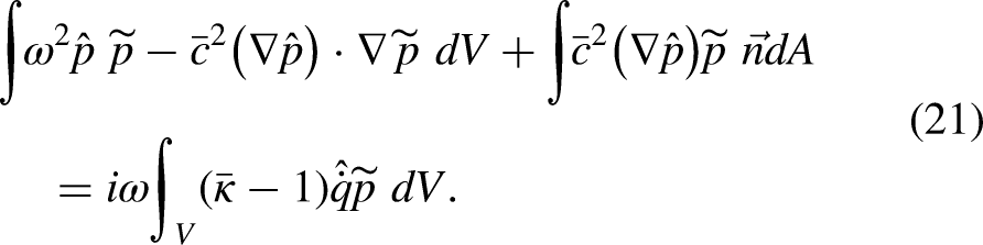
Hybrid CFD/CAA modelling is one approach to solve the inhomogeneous wave equation by the separation of the mean flow field and the aeroacoustic domain. The acoustic response is solved numerically in COMSOL employing the local quasi-steady convective flame response model. In order to solve the inhomogeneous wave equation in the Galerkin FEM framework, the weak formulation of equation (5) including the flame response model coupled to the acoustic pressure is used

$$\begin{array}{rl}& \int {\omega }^2\hat{p}\tilde{p}-{\overline{c}}^2\left(\mathrm{\nabla }\hat{p}\right)\cdot \mathrm{\nabla }\tilde{p}dV+\int {\overline{c}}^2\left(\mathrm{\nabla }\hat{p}\right)\tilde{p}\overrightarrow{n}dA\\ & =i\omega {\int }_V(\overline{\kappa }-1)\hat{\dot{q}}\tilde{p}dV\end{array}$$

(21)

The test function is denoted with $\tilde{p}$ , for details on the derivation we refer to Heilmann et al. ²⁷ The compression model according to equation (10) is directly coupled to the acoustic pressure field. However, the displacement and the convective model require the acoustic velocity in the entire field and at the reference position $x_{\mathrm{ref}}$ , respectively. The momentum conservation yields $\hat{u}=-\frac{1}{i\omega \rho }\frac{\mathrm{\partial }\hat{p}}{\mathrm{\partial }x}$ neglecting mean flow effects on the acoustics. The more restrictive thin flame assumption in the LF case^6,20,19 is not valid anymore for higher frequencies even if the wave propagation remains longitudinal. Therefore, the axially distributed flame response model accounts for the convective non-compactness of the local FTF.

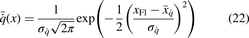
In first proximity, the mean heat release distribution is assumed constant in the cross-sectional direction $\overline{\dot{q}}\ne f(r,\phi )$ . For the axial direction a Gaussian heat release distribution

$$\overline{\dot{q}}\left(x\right)=\frac{1}{{\sigma }_{\dot{q}}\sqrt{2\pi }}\exp \left(-\frac{1}{2}{\left(\frac{x_{\mathrm{Fl}}-{\overline{x}}_{\dot{q}}}{{\sigma }_{\dot{q}}}\right)}^2\right)$$

(22)

with the variance ${\sigma }_{\dot{q}}$ and the axial ‘centre of gravity’ of the flame ${\overline{x}}_{\dot{q}}$ is accounted for using the axial coordinate of the flame $x_{\mathrm{Fl}}=x-x_{\mathrm{ref}}$ , see Figure 1. The constant convection velocity from the injector exit to the flame front is defined equal to the injector tube velocity times a constant $Y_u\propto 1$ representing the reduction in flow velocity due to the mixing of the unburned and burned gas. The hybrid CFD/CAA model might be generalised to include a mean velocity field from CFD accounting for the convective wave numbers in all directions of space. However, in the present work a straight flow path from the reference plane to the flame front is assumed aligned with the axial direction to apply equation (20). The numerical model is used in the following to access the pressure field in the injector tubes and to verify the transfer matrix reconstruction and the low-order network model discussed in the next section.

Network model

Low-order network models provide physical insights on thermoacosutic systems and efficient predictive tools for the early design phase of combustors. Therefore, a low-order network model is provided in the following extending the two-port network modelling approach to HF thermoacoustics.

Duct transfer matrix

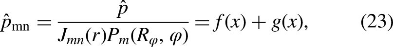
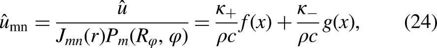
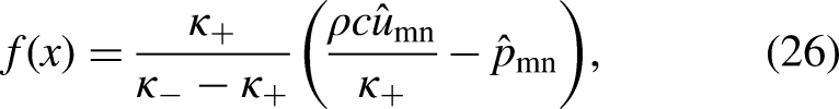
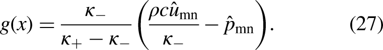
The main idea is to use of the similarity in the separation ansatz functions for the acoustic pressure and axial acoustic velocity in cylindrical combustion chambers. Momentum conservation neglecting mean flow effects or dissipation yields the simple relation of the axial acoustic velocity by the gradient of the acoustic pressure. Thus, the radial and azimuthal dependency of acoustic pressure and axial velocity are self-similar. Normalisation with the radial Bessel and azimuthal ansatz function $J_{mn}(r)$ , $P_m(\phi )=e^{-im\phi }+R_{\phi }{e}^{im\phi }$ , respectively, yields

$${\hat{p}}_{\mathrm{mn}}=\frac{\hat{p}}{J_{mn}(r)P_m(R_{\phi },\phi )}=f(x)+g(x)$$

(23)

$${\hat{u}}_{\mathrm{mn}}=\frac{\hat{u}}{J_{mn}(r)P_m(R_{\phi },\phi )}=\frac{{\kappa }_{+}}{\rho c}f(x)+\frac{{\kappa }_{-}}{\rho c}g(x)$$

(24)

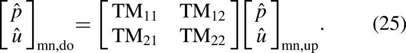
which are reffered to as effective modal acoustic pressure and axial velocity, since the normalisation depends on the mode number in radial and azimuthal direction. Thus, only the axial dependency on the downstream and upstream travelling f- and g-wave $f(x)=\hat{f}{e}^{-i{k}_{+}x}$ and $g(x)=\hat{g}{e}^{-i{k}_{-}x}$ is considered. For a compact notation the axial wave numbers $k_{\pm }=\pm \sqrt{k^2-k_{mn}^2}$ and the normalised axial wave numbers ${\kappa }_{\pm }=\frac{k_{\pm }}{k}$ are introduced. The wave number of the Bessel function $k_{mn}=\frac{{\alpha }_{mn}}{r}$ is defined by the argument of the Bessel function at its maximum for instance at the T1 mode ${\alpha }_{mn}=1.841$ . Note that the amplitudes in azimuthal direction are included in the amplitudes $\hat{f}$ and $\hat{g}$ by the parametrisation with the azimuthal reflection coefficient $R_{\phi }=\frac{g_{\phi }}{f_{\phi }}$ and the use of the Bessel function implies rigid wall boundary conditions at the combustor wall in the radial direction. The effective acoustic pressure $p_{\mathrm{eff}}^{\prime }$ and effective axial acoustic velocity $u_{\mathrm{eff}}^{\prime }$ up- and downstream of a duct, an area change or a flame can thus be described by a two-port transfer matrix

$${\left[\begin{array}{c}\hat{p}\\ \hat{u}\end{array}\right]}_{\mathrm{mn},\mathrm{do}}=\left[\begin{array}{cc}{\mathrm{TM}}_{11}& {\mathrm{TM}}_{12}\\ {\mathrm{TM}}_{21}& {\mathrm{TM}}_{22}\end{array}\right]{\left[\begin{array}{c}\hat{p}\\ \hat{u}\end{array}\right]}_{\mathrm{mn},\mathrm{up}}$$

(25)

Equivalent scattering matrices for the f- and g-waves might be derived using

$$f(x)=\frac{{\kappa }_{+}}{{\kappa }_{-}-{\kappa }_{+}}(\frac{\rho c{\hat{u}}_{\mathrm{mn}}}{{\kappa }_{+}}-{\hat{p}}_{\mathrm{mn}})$$

(26)

$$g(x)=\frac{{\kappa }_{-}}{{\kappa }_{+}-{\kappa }_{-}}(\frac{\rho c{\hat{u}}_{\mathrm{mn}}}{{\kappa }_{-}}-{\hat{p}}_{\mathrm{mn}})$$

(27)

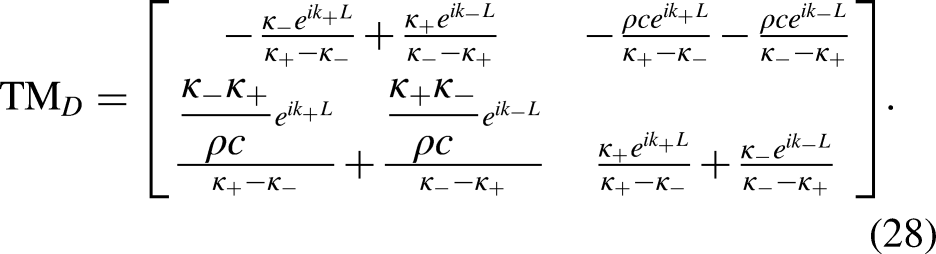
The acoustic transfer matrix of a HF duct is derived from the solution of the Bessel differential equation for the effective acoustic pressure equation (23) and axial acoustic velocity equation (24) expressed via the up- and downstream travelling f- and g-wave upstream of the duct $x=0$ and downstream of the duct $x=L$ , which yields

$${\mathrm{TM}}_D=\left[\begin{array}{cc}-\frac{{\kappa }_{-}{e}^{i{k}_{+}L}}{{\kappa }_{+}-{\kappa }_{-}}+\frac{{\kappa }_{+}{e}^{i{k}_{-}L}}{{\kappa }_{-}-{\kappa }_{+}}& -\frac{\rho c{e}^{i{k}_{+}L}}{{\kappa }_{+}-{\kappa }_{-}}-\frac{\rho c{e}^{i{k}_{-}L}}{{\kappa }_{-}-{\kappa }_{+}}\\ \frac{\frac{{\kappa }_{-}{\kappa }_{+}}{\rho c}{e}^{i{k}_{+}L}}{{\kappa }_{+}-{\kappa }_{-}}+\frac{\frac{{\kappa }_{+}{\kappa }_{-}}{\rho c}{e}^{i{k}_{-}L}}{{\kappa }_{-}-{\kappa }_{+}}& \frac{{\kappa }_{+}{e}^{i{k}_{+}L}}{{\kappa }_{+}-{\kappa }_{-}}+\frac{{\kappa }_{-}{e}^{i{k}_{-}L}}{{\kappa }_{-}-{\kappa }_{+}}\end{array}\right]$$

(28)

Assuming a low Mach number simplifies the transfer matrix using $\frac{{\kappa }_{\pm }}{{\kappa }_{\mp }-{\kappa }_{\pm }}=-\frac{1}{2}$ to a very similar transfer matrix as used for LF axial modes can annular combustors.^17,16 Thus, the longitudinal wave propagation in the injector tubes is included in equation (28) setting the argument of the Bessel function to ${\alpha }_{mn}=0$ , which yields the wave number $k_{\pm }=\pm k$ in the low Mach limit.

The derivation of the transfer matrix of an acoustic area jump or across a flame, however, is not as straightforward as the duct transfer matrix and requires cross-sectional integrated conservation equations as considered in the next section.

Integral HF acoustic jump conditions

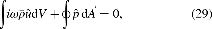
The derivation of acoustic jump conditions are generally based on the choice of proper integral conservation equations. The linearised momentum conservation (equation (2)) in the low Mach number limit is commonly used to obtain the acoustic pressure coupling condition for acoustic network elements

$$\int i\omega \overline{\rho }\hat{u}\mathrm{d}V+\oint \hat{p}\mathrm{d}\overrightarrow{A}=0$$

(29)

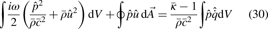
In the context of LF acoustics, the linearised mass conservation is predominantly used for the acoustic velocity transfer function across area changes, while linearised energy conservation is common for LF thermoacoustic jump conditions across flames. Both linearised mass and energy conservation result in the conservation of volume velocity, expressed as $\oint u_x^{\prime },\mathrm{d}\overrightarrow{A}=\mathrm{const}.$ across area changes and flames. However, as indicated by Pierce et al., ³⁴ the acoustic power flux $p^{\prime }{u}^{\prime }$ has to be employed to obtain the correct acoustic jump conditions. Yet, in the LF limit, the acoustic power transmitted across a sudden area expansion reduces to the same volume velocity jump condition as previously mentioned. In the HF case, however, the cross-sectional non-compactness of the acoustic field has to be accounted. Thus, the acoustic disturbance energy conservation yields a suitable jump condition since it covers the transmitted acoustic power across sudden area expansions and non-compact flame driving, which is crucial in the HF regime. Concerning the acoustic velocity transfer function the integral disturbance energy conservation

$$\int \frac{i\omega }{2}(\frac{{\hat{p}}^2}{\overline{\rho }{\overline{c}}^2}+\overline{\rho }{\hat{u}}^2)\mathrm{d}V+\oint \hat{p}\hat{u}\mathrm{d}\overrightarrow{A}=\frac{\overline{\kappa }-1}{\overline{\rho }{\overline{c}}^2}\int \hat{p}\hat{\dot{q}}\mathrm{d}V$$

(30)

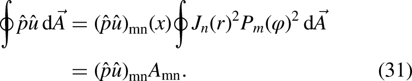
is employed, with the restriction to low Mach numbers. The acoustic power flux in the disturbance energy conservation is separated into the axial, radial, and azimuthal dependency of the acoustic field considering can-combustors. Therefore, the acoustic field is expressed via the modal acoustic pressure and axial velocity using equations (23) and (24), which yields for the acoustic power flux

$$\oint \hat{p}\hat{u}\mathrm{d}\overrightarrow{A}=(\hat{p}\hat{u}{)}_{\mathrm{mn}}(x)\oint J_n{(r)}^2{P}_m(\phi {)}^2\mathrm{d}\overrightarrow{A}=(\hat{p}\hat{u}{)}_{\mathrm{mn}}{A}_{\mathrm{mn}}$$

(31)

The effective modal cross-sectional area is introduced

$$A_{\mathrm{mn}}=\int J_n{(r)}^2{P}_m(\phi {)}^2\mathrm{d}A$$

(32)

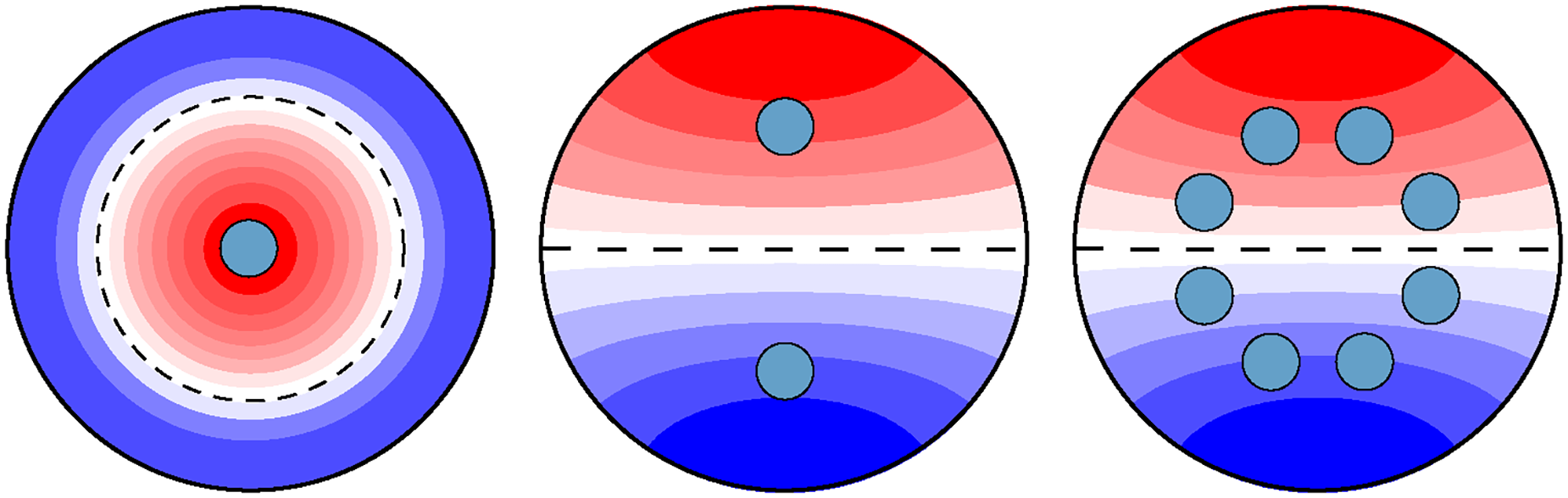
which simplifies the notation of the acoustic power flux. The integral ${\int }_A{J}_n{(r)}^2{P}_m(\phi {)}^2\mathrm{d}A$ is reffered to as effective modal area since the cross-sectional area is effectively reduced by the radial and azimuthal dependency $J_n(r),P_m(\phi )$ , which are non-dimensional. Equation (31) considers only the acoustic power transmitted in axial direction, since the acoustic power transmitted across transverse nodal lines or at fully reflective walls is zero. Consequently, HF modes can be segregated into multiple acoustic domains in the cross-sectional direction at transverse/radial nodal lines and wall boundary conditions, as depicted in Figure 2. Thus, the integration boundaries in radial and azimuthal directions of the effective modal acoustic area have to be properly chosen by the regions separated by the transverse/radial nodal lines and the combustor wall, as indicated by the dashed and solid lines in Figure 2, respectively, considering three jet combustor configurations. The central injector tube couples solely to the effective area between $r=0$ to $r=0.63R$ indicated by the dashed line in Figure 2 on the left side. Consequently, four injector tubes couple to the upper/lower half for the depicted case of the T1 mode depicted at the right side of Figure 2. Concerning the radial direction the integration boundaries $r_{\min }$ and $r_{\max }$ are determined at the extrema of the Bessel function and the nodal line position $J_{mn}(r)=0$ . The azimuthal direction is separated at the integration boundaries ${\phi }_{\min }=-\pi /2^m$ and ${\phi }_{\min }=+\pi /2^m$ . Considering MJCs the effective modal acoustic area of the injector tubes within each domain according toequation (32) is simplified assuming compactness of the injector tube diameter to the local transverse/radial acoustic mode shape. In this case, equation (32) simplifies to the discretised sum of the geometrical injector tube area $A_T$ weighted with the radial and azimuthal ansatz function $A_{\mathrm{mn}}=\sum _i{A}_{T}J(r_T)P({\phi }_T)$ at the injector tube position $r_T,{\phi }_T$ .

Figure 2.

Effective modal cross-sectional areas separated by the transverse nodal lines and wall boundary conditions for the R1 and T1 mode and different injector tube configurations coupling to the high frequency (HF) mode at the dump plane.

The next sections provide the thermoacoustic network elements covering a straight duct, a sudden area expansion and a flame, making use of the integral conservation equations according to equations (29) and (30).

Area change transfer matrix

Considering acoustic compactness ${\mathrm{He}}_x\ll 1$ in the axial direction might be reasonable especially close to the cut on frequency for a sudden area expansion. In this case, the first terms on the left-hand side of equations (29) and (30) covering the acoustic inertia (i.e. the effective length scale) and the unsteady change in acoustic energy in the control volume (i.e. the reduced length scale) are neglected. Therefore, the integral conservation of acoustic momentum and disturbance energy read

$${\hat{p}}_{\mathrm{mn},\mathrm{do}}={\hat{p}}_{\mathrm{mn},\mathrm{up}}$$

(33)

$$(\hat{p}\hat{u}A{)}_{\mathrm{mn},\mathrm{do}}=(\hat{p}\hat{u}A{)}_{\mathrm{mn},\mathrm{up}}$$

(34)

For an axially compact area expansion, the transmitted acoustic power reduces to the ratio of the modal acoustic cross-sectional areas since the modal acoustic pressure remains constant, which yields the area jump transfer matrix

$${\mathrm{TM}}_A=\left[\begin{array}{cc}1& 0\\ 0& \frac{A_{\mathrm{mn},\mathrm{up}}}{A_{\mathrm{mn},\mathrm{do}}}\end{array}\right]$$

(35)

The effective tube length due to the acoustic inertia might still be considered via an effectively elongated tube length in the duct transfer matrix. Alternatively, the effective length is obtained from the volume integral on the left-hand side of the momentum conservation equation (29) assuming axial compactness of the acoustic velocity mode shape which yields

$$-i\omega \overline{\rho }{\hat{u}}_{\mathrm{mn},\mathrm{up}}{L}_{\mathrm{eff}}{A}_{\mathrm{mn},\mathrm{up}}=-{\int }_{V}i\omega \overline{\rho }\hat{u}\mathrm{d}V$$

(36)

The non-compact area change transfer matrix neglecting the reduced length scale yields

$${\mathrm{TM}}_A=\left[\begin{array}{cc}1& -i\omega \overline{\rho }{L}_{\mathrm{eff}}\\ 0& \frac{A_{\mathrm{mn},\mathrm{up}}}{A_{\mathrm{mn},\mathrm{do}}}\end{array}\right]$$

(37)

Similar a reduced length ³⁵ might be accounted for in the disturbance energy conservation equation (30). For the investigated MJC configuration, the sudden 90 $\circ$ transition from injector section to combustion chamber yields negligible reduced length scales. The considered effective length scale of $L_{\mathrm{eff}}=0.611d_T/2$ due to the acoustic inertia, however, decreases the eigenfrequencies dependend on the injector tube diameter.

Flame transfer matrix (FTM)

In order to obtain the FTM including a non-compact FTF, the momentum and disturbance energy conservation is considered

$${\hat{p}}_{\mathrm{mn},\mathrm{b}}={\hat{p}}_{\mathrm{mn},\mathrm{u}}$$

(38)

$$(\hat{p}\hat{u}A{)}_{\mathrm{mn},b}=(\hat{p}\hat{u}A{)}_{\mathrm{mn},u}(1+\frac{{\int }_V\frac{\overline{\kappa }-1}{\overline{\kappa }\overline{p}}\hat{p}\hat{\dot{q}}\mathrm{d}V}{(\hat{p}\hat{u}A{)}_{\mathrm{mn},u}})$$

(39)

The restriction to a flame in a straight duct implies negligible acoustic inertia in the momentum equation. Further, a quasi-steady disturbance energy in the control volume is assumed. Thus, the volume integral on the left-hand side, which covers the storage of acoustic energy in the control volume, is omitted. The coupling condition according to equation (39) is further simplified by the use of ${\hat{p}}_{\mathrm{mn},\mathrm{b}}/{\hat{p}}_{\mathrm{mn},\mathrm{u}}=1$ according to equation (38). The factor $\frac{\overline{\kappa }-1}{\overline{\kappa }\overline{p}}$ is commonly expressed via the temperature ratio assuming constant gas properties. ³⁶ The heat capacity ratio ${\overline{c}}_p=\overline{\kappa }{\overline{c}}_v$ and the ideal gas law ${\overline{\rho }}_u{\overline{T}}_u=\frac{\overline{p}}{R_u}$ are used to express the mean heat release rate $\overline{\dot{Q}}={\overline{\rho }}_u{\overline{u}}_u{A}_u{\overline{c}}_p({\overline{T}}_b-{\overline{T}}_u)$ . Finally, the FTM reads

$$\mathrm{FTM}=\left[\begin{array}{cc}1& 0\\ 0& (1+(\frac{{\overline{T}}_b}{{\overline{T}}_u}-1)\mathrm{FTF})\end{array}\right]$$

(40)

including the FTF given by

$$\mathrm{FTF}=\frac{{\int }_V\hat{p}\hat{\dot{q}}\mathrm{d}V/\overline{\dot{Q}}}{(\hat{p}\hat{u}A{)}_{\mathrm{mn},u}/(\overline{u}A{)}_u}$$

(41)

The Rayleigh integral is normalised by the modal acoustic pressure at unburned conditions ${\hat{p}}_{\mathrm{mn},u}$ which is spatially invariant. The acoustic pressure field is expressed via the non-dimensional axial acoustic mode shape

$${\hat{\mathrm{\Pi }}}_x=\frac{{\hat{p}}_{\mathrm{mn}}(x)}{{\hat{p}}_{\mathrm{mn},u}}$$

(42)

for convinience. Thus, the non-compact coupling of the heat release rate fluctuations and the acoustic pressure in the FTF according to equation (41) is rewritten as

$$\mathrm{FTF}=\frac{{\int }_V{J}_n{P}_m{\hat{\mathrm{\Pi }}}_x\hat{\dot{q}}\mathrm{d}V/\overline{\dot{Q}}}{(\hat{u}A{)}_{\mathrm{mn},u}/(\overline{u}A{)}_u}$$

(43)

where the volume integral ${\int }_V{J}_n{P}_m{\hat{\mathrm{\Pi }}}_x\hat{\dot{q}}\mathrm{d}V$ can be interpreted as a weighted integral heat release with respect to the non-dimensional acoustic pressure mode shape. The FTF can either be modelled analytically or equation (40) is used to reconstruct the flame transfer matrix from CFD employing RANS or LES simulations or forced response experiments. The reconstruction of the FTM according to equation (40) is demonstrated in the ‘Flame transfer matrix and function’ section using the hybrid CFD/CAA model. A suitable simplified analytical model is proposed in the next section.

Analytical FTF

A general analytical FTF might be obtained by integration of the unsteady heat release rate fluctuations including flame compression, flame displacement, reaction rate fluctuations and possible other coupling mechanisms. However, the following analysis focuses solely on the convective contribution due to coherent turbulent velocity fluctuations at the flame.

Consider a MJC with multiple injector tubes of the same diameter and length flush-mounted in a planar front plate. The overall mass flow is split equally to each jet flame resulting in similar fluiddynamical conditions at each flame. Concerning negligible flame-flame interaction, a symmetric flame stabilisation results in a constant consumption rate at each flame in cross-sectional direction. The local flame response model (equation (20)) accounts for an axially resolved local flame response and is applied to the volume integral in equation (43) considering an axially acoustic compact flame ${\hat{\mathrm{\Pi }}}_x=1$ . A Gaussian heat release distribution equation (22) along with equation (43) yields an equivalent spatial formulation

$$\mathrm{FTF}=n{e}^{-i{k}_{\mathrm{conv}}{\overline{x}}_{\dot{q}}}{e}^{-\frac{1}{2}(k_{\mathrm{conv}}{\sigma }_{\dot{q}}{)}^2}$$

(44)

of the $n-\tau -\sigma$ time delay model ³ for the effective acoustic velocity in the HF regime. The phase lag of the FTF according to equation (44) is determined by the mean convective wave number and the axial ‘centre of gravity’ of the flame ${\overline{x}}_{\dot{q}}$ . The relation ${\overline{\tau }}_{\dot{q}}={\overline{x}}_{\dot{q}}/\overline{u}$ yields the analogous formulation with a mean time delay $k_{\mathrm{conv}}{\overline{x}}_{\dot{q}}=\omega {\overline{\tau }}_{\dot{q}}$ . The product of spatial variance and convective wave number in equation (44) is equivalent to the variance in time delay $k_{\mathrm{conv}}{\sigma }_{\dot{q}}={\sigma }_{\tau }$ , which determines the decreasing slope of the gain for increasing frequency. This low -pass behaviour of the gain, might lead to the intuitive conclusion that the integral convective heat release fluctuations are negligible in the HF regime. However, the decreasing gain might be over-compensated by an increasing flow velocity or decreasing flame length due to the Strouhal number dependency of equation (44). The scaling of the FTF might be expressed via the Strouhal number $\mathrm{St}=\frac{L_{\mathrm{Fl}}}{{\lambda }_{\mathrm{conv}}}=f\frac{L_{\mathrm{Fl}}}{\overline{u}},$ obtained from the axial flame length in relation to the convective wavelength. The variance might be expressed as a fraction $a_{\sigma }=\mathcal{O}(1)$ of the entire flame length ${\sigma }_{\dot{q}}=a_{\sigma }{L}_{\mathrm{Fl}}$ and the convective wave number as $k_{\mathrm{conv}}=\frac{\omega }{\overline{u}}$ , which yields $\mathrm{FTF}\propto e^{-\frac{1}{2}(a_{\sigma }2\pi \mathrm{St}{)}^2}.$ The Strouhal number represents the number of $\pi$ phase changes of the heat release rate fluctuations in axial direction, which lead to a decreasing gain with increasing frequency. At the same frequency, but for increasing axial mean flow the convective wave length in axial direction increases and thus the number of phase changes of the heat release rate within the flame length decreases and the gain increases proportional to the change in the Strouhal number. However, the dependency of the FTF gain on the Strouhal number in equation (44) emphasizes that operating conditions and injector design influencing the ratio of flame length to convective wave length is a parameter as crucial as the cut on frequency of the HF mode for the low-pass behaviour. Consequently, short flame lengths and high convection velocities as well as low cut on frequencies due to, that is, large combustor diameters might overcompensate the low-pass behaviour of the flame response at higher frequencies leading to HF combustion instabilities.

Validation of the HF flame response

The convective flame model is validated with a flame response experiment forcing the T1 mode in a multi-jet combustor ¹⁰ and an equivalent numerical model employing the inhomogeneous wave equation. The perfectly premixed unburned natural gas and air mixture enters the plenum via a perforated plate with a low Mach number, see Figure 3. The flow splits into a pilot mass flow and a jet flame mass flow with a pilot mass fraction of $Y_{\mathrm{pilot}}=0.1$ . In the combustion chamber, a T1 mode is forced via two Monacor KU-516 driver, one driver at the top and one at the bottom. Note that a negligible cooling purge flow is used. Optical access is assured over the full flame length in the optical section using a quartz glass flame tube to measure the flame response by $\mathrm{OH}*$ chemiluminescence. Afterwards, the exhaust gas flows through a metallic combustion chamber with pressure sensors ${\mathrm{C}}_1$ and ${\mathrm{C}}_2$ at the top of the chamber. Four additional pressure sensors are mounted at the top and the bottom of the front plate ${\mathrm{FP}}_1-{\mathrm{FP}}_4$ . The measured heat release rate fluctuations are phase-locked using pressure sensor ${\mathrm{C}}_1$ close to the flames downstream of the forcing inlets. A minimum of 500 images per each of the eight phase bins $n_{\mathrm{bin}}=8$ is used to eliminate stochastic, turbulent fluctuations. ¹⁰ The operating conditions are summarised in Table 1.

Figure 3.

Experimental setup for the integrated OH $*$ images and the simultaneous pressure measurements at four positions in the front plate ${\mathrm{FP}}_1-{\mathrm{FP}}_4$ and two in the combustor ${\mathrm{C}}_1$ and ${\mathrm{C}}_2$ .

Table 1.

Operating conditions.

${\lambda }_{\mathrm{NG}}$	$T_u$	$T_b$	$Y_{\mathrm{pilot}}$	${\dot{m}}_{\mathrm{air}}$	$P_{\mathrm{th}}$
1.5	673 K	2070 K	0.1	120 g s−1	230 kW

The MJC is modelled numerically as depicted in Figure 4, in order to apply the thermoacoustic coupling models using the hybrid CFD/CAA method. The mean temperature field is simplified to a constant preheat temperature in the plenum, the injector tubes, the swirl stabilised pilot burner and the unburned core region of the flames of $T_u=673$ K. Downstream of the flames in the combustion chamber the estimated adiabatic flame temperature of $T_b=2070$ K is applied, see also Table 1. The thermal power for each of the eight flames subtracting the thermal power of the pilot burner with a mass fraction of 10% yields the thermal power of $P_{\mathrm{th},\mathrm{Jet}}=207$  kW. The Gaussian distribution of the thermal power in the axial direction as well as the mean axial velocity used for the convective wave number in the numerical model is fitted to the experimental data. Impedance boundary conditions representing the low Mach number perforated plate $z_{\mathrm{up}}=2$ and the measured reflective boundary condition downstream of the combustor $z_{\mathrm{do}}=100$ are used. The swirl-stabilised pilot burner might introduce a spin to the T1 mode in the forced response experiment. However, as shown by Rosenkranz et al. ¹⁰ the applied forcing yields spin ratios very close to zero and a constant nodal line position between the top and the bottom half of the combustor. Thus, the azimuthal reflection coefficient is set to unity in the numerical model corresponding to a standing mode in the transverse direction.

Figure 4.

Mean speed of sound [ms⁻¹] (top) and mean heat release rate density [Wm⁻³] (bottom) of the numerical Helmholtz model considering a preheat temperature of $T_u=673$  K and an adiabatic flame temperature of $T_b=2070$  K.

The resulting pressure mode shape in Figure 5 confirms the strong axial acoustic velocity, that is, strong axial acoustic pressure gradients, at the injector exit at the investigated injector tube length and operating condition. The relatively weak and evanescent T1 mode shape in the combustion chamber suggests that the flame response due to the strong injector coupling is the dominant effect and flame displacement and compression can be discarded.

Figure 5.

The resulting acoustic pressure mode shape [Pa] (top) and the convective heat release rate density fluctuations [Wm⁻³] (bottom) of the numerical Helmholtz model at 3100 Hz considering a preheat temperature of $T_u=673$  K and an adiabatic flame temperature of $T_b=2070$  K.

The flame response is modelled using the hybrid CFD/CAA method, as depicted in Figure 5. Despite the rough simplification of the mean heat release field in Figure 4, the numerical results reveal the axial pattern of the heat release fluctuations and also cover the dependency of the amplitude on the Bessel function, since the jet flames in the centre show a lower amplitude compared to the jet flames close to the walls. The axial pattern in heat release fluctuations caused by axial acoustic velocity fluctuations at the dump plane determine the phase and the gain of the resulting global flame transfer function, see equation (44). Thus, the model captures the main physical contribution of the convective driving mechanism to the flame response similar to common hybrid CFD/CAA models^20,19,4 with a locally resolved flame response and the possibility to include a mean CFD field.

A detailed validation of the axially resolved, convective FTF at a single radial position in the phase-locked image at the top flames close to the combustor wall is considered, indicated by the upper dashed line in Figure 6. The results of the model and the experiment show the unsteady and mean heat release rates for a single phase $\phi =0$ in the oscillation, see Figure 6. According to equation (20), the flame response is determined by the axial acoustic velocity, the axial convective wave number and the mean heat release, which is fitted to a Gaussian distribution. In the absence of acoustic pressure measurements in the injector tube, the axial acoustic velocity amplitude at the reference position is reconstructed from the numerical model fitted to the measured pressure sensor data, see Figure 5. The numerically fitted acoustic pressure field in Figure 5 yields a normalised fluctuation of ${\hat{u}}_{\mathrm{ref}}/{\overline{u}}_{\mathrm{ref}}\approx 0.055e^{i\cdot \mathrm{\angle }{\hat{u}}_{\mathrm{ref}}}$ and a gain of approximately $n=1.1$ , which results in a good agreement of the experimental and analytical heat release rate fluctuations. The phase angle of the axial acoustic velocity amplitude ${\hat{u}}_{\mathrm{ref}}$ at the reference position is obtained from the numerical model by $\mathrm{\angle }{\hat{u}}_{\mathrm{ref}}=\mathrm{\angle }{\hat{u}}_{\mathrm{ref}}-\mathrm{\angle }{\hat{p}}_{C_1}=2.3$ rad accounting for the difference of the axial velocity to the complex acoustic pressure at the sensor position $C_1$ , since the flame response is phase-locked to pressure sensor $C_1$ . The fitted convection velocity of the heat release patches yields lower values compared to the velocity in the injector tubes. The results shown in Figure 6 are in good agreement with a unburned gas mixture fraction at the flame front of $Y_u=0.88$ close to unity, thus 12% lower convection velocity. The normalised amplitudes in heat release oscillation $\frac{{\dot{q}}^{\prime }}{\overline{\dot{q}}}$ is preserved in the axial direction for the shown case of $T_u=673$  K and ${\lambda }_{{\mathrm{CH}}_4}=1.5$ , which might be due to the close vicinity of the coherent vortices to the jet core region. The low dissipation of the heat release rate fluctuations in the axial direction along the flames confirms the coherent vortex velocity transport model according to equation (15) in the high Reynolds number limit, that is, the transport of ${\hat{u}}_v$ is properly modelled by the Euler equation.

Figure 6.

Forced flame response for $\phi =0$ at a preheat temperature of $T_u=673$  K and an air excess ratio of ${\lambda }_{{\mathrm{CH}}_4}=1.5$ at 3100 Hz of the MJC with pilot burner (left) and the comparison of the experimental flame response ( $◻$ ) to the flame response model ( $-$ ) (right) at the upper flames, indicated by the dashed line.

The axially resolved flame response model accounting solely for the acoustic velocity fluctuations is highly consistent with the experimental flame response. Further validation of the axial acoustic velocity at the injector tube exit is in progress.

Validation of the HF transfer matrices

The results for the non-reactive and reactive transfer matrices are presented in the following sections, extending the two port transfer matrix method to the HF regime. First, the transfer matrix reconstruction methodology is provided. Second, the non-reactive, purely acoustic transfer matrices are validated by a generic, non-reactive experiment. Third, the results concerning the flame transfer matrix are verified with the numerical hybrid CFD/CAA model.

Transfer matrix reconstruction

The model verification and validation with numerical and experimental results is based on the reconstruction of the proposed quasi-two-port transfer matrices in the HF regime, discussed in this section. The multi-microphone-method (MMM) in the axial, the radial and the azimuthal directions is common practise to analyse HF thermoacoustic instabilities.^38,37 The reconstruction of transfer or scattering matrices, however, is cumbersome since various unknowns of the multi-port coupling are to be determined.^40,39 Therefore, the effective acoustic pressure equation (23) and axial acoustic velocity equation (24) normalised with the radial and azimuthal dependencies are used to obtain a quasi-two-port transfer matrix reconstruction for HF acoustics. The spin ratio $\mathrm{SR}$ or azimuthal reflection coefficient $R_{\phi }$ , however, needs to be determined for the normalisation in equations (24) and (23) from the MMM in the azimuthal direction.

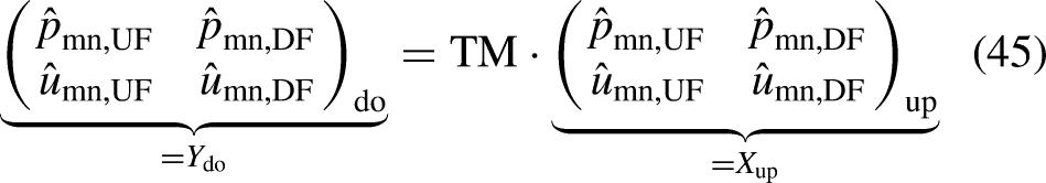
The two-source location method with upstream forcing (UF) and downstream forcing (DF)

$$\underset{=Y_{\mathrm{do}}}{\underbrace{{\left(\begin{array}{cc}{\hat{p}}_{\mathrm{mn},\mathrm{UF}}& {\hat{p}}_{\mathrm{mn},\mathrm{DF}}\\ {\hat{u}}_{\mathrm{mn},\mathrm{UF}}& {\hat{u}}_{\mathrm{mn},\mathrm{DF}}\end{array}\right)}_{\mathrm{do}}}}=\mathrm{TM}\cdot \underset{=X_{\mathrm{up}}}{\underbrace{{\left(\begin{array}{cc}{\hat{p}}_{\mathrm{mn},\mathrm{UF}}& {\hat{p}}_{\mathrm{mn},\mathrm{DF}}\\ {\hat{u}}_{\mathrm{mn},\mathrm{UF}}& {\hat{u}}_{\mathrm{mn},\mathrm{DF}}\end{array}\right)}_{\mathrm{up}}}}$$

(45)

yields the transfer matrix in $p,u$ -notation

$$\mathrm{TM}=X_{\mathrm{up}}^{-1}{Y}_{\mathrm{do}}$$

(46)

from the effective acoustic pressure and axial velocity up and do of the transfer element obtained with the MMM.

Acoustic transfer matrices

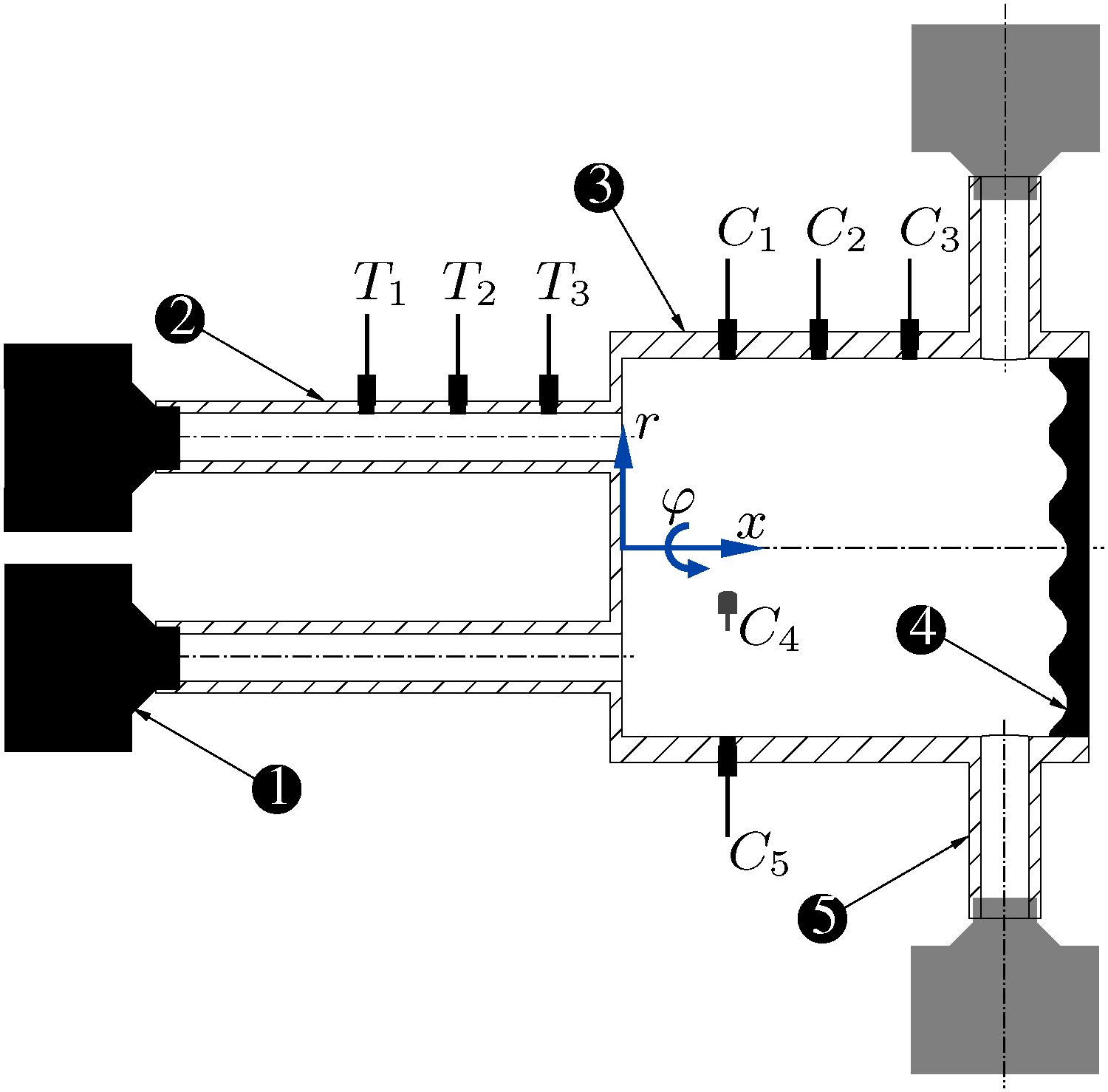
To step-wise increase the complexity, first the purely acoustic transfer matrices are validated with experimental results of a generic experiment with two ducts coupled to a cylindrical chamber, see Figure 7. The dynamic pressure sensors at three positions in the Tube $T_1-T_3$ and the chamber $C_1-C_3$ are used to perform the MMM in the axial direction. The additional sensors $C_4-C_5$ together with $C_1$ yield the azimuthal reflection coefficient of unity or the equivalent spin ratio of zero, which implies a perfectly standing mode shape in transverse direction. Thus, the assumption of a constant spin ratio of zero in the analytical and the numerical model is valid.

Figure 7.

Generic experimental setup to validate the acoustic transfer matrices with a forced response of the T1 mode using counterwise upstream and downstream forcing at positions (1) and (5) and pressure sensors at positions $T_1-T_3$ in the tube and $C_1-C_5$ in the cylindrical chamber.

The low and high frequency wave propagation in the tubes and the chamber is known from acoustic theory, ³⁵ which is extended by the HF acoustic area jump condition at the interface of tube and chamber according to equation (37). The resulting analytical transfer matrix from upstream of the tubes to downstream of the chamber

$$\mathrm{TM}={\mathrm{TM}}_T{\mathrm{TM}}_{T/C}{\mathrm{TM}}_C$$

(47)

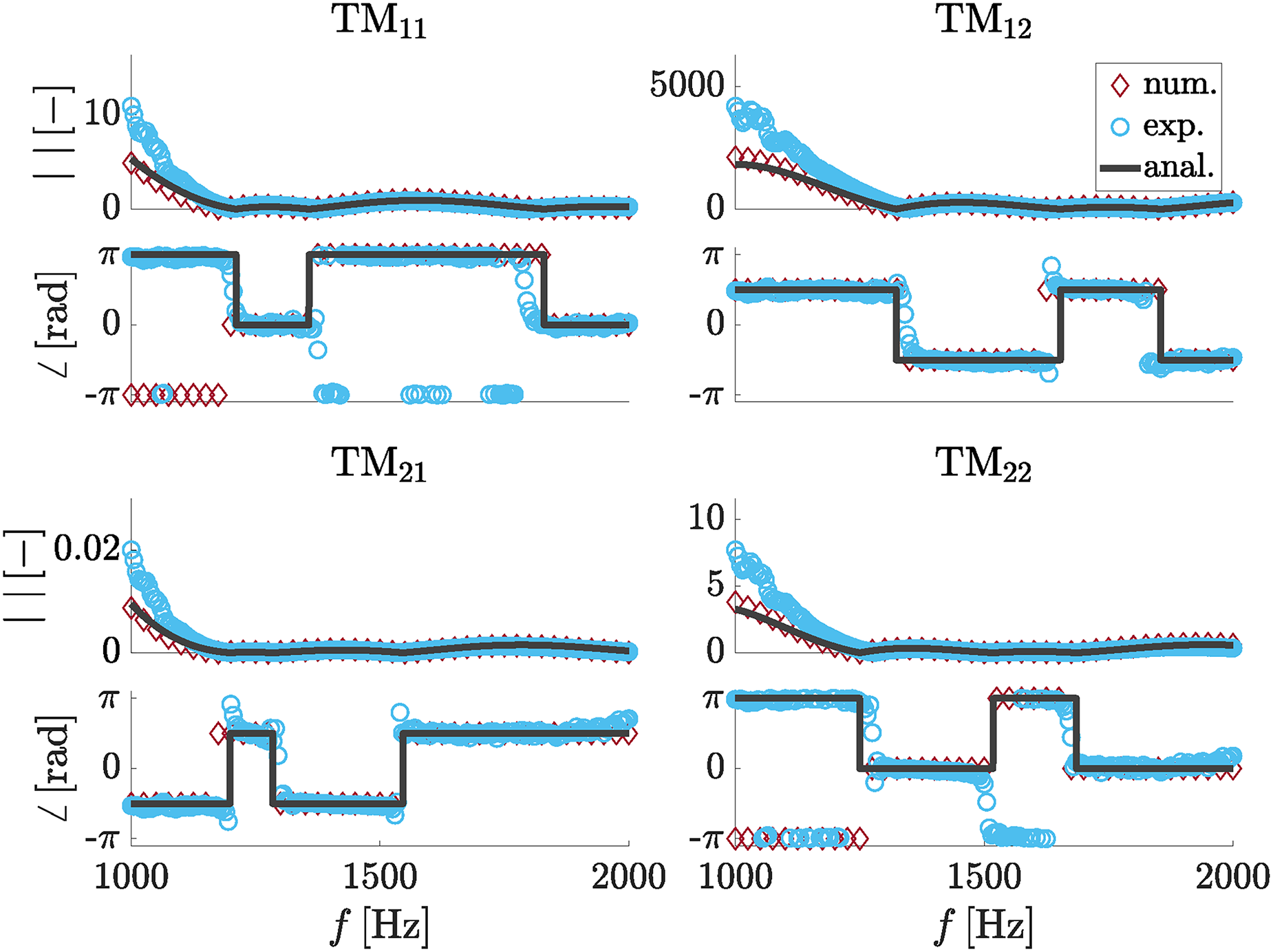
covering the longitudinal acoustic wave propagation in the tube ${\mathrm{TM}}_T$ , the tube-chamber area jump ${\mathrm{TM}}_{T/C}$ and the T1 mode wave propagation in the chamber ${\mathrm{TM}}_C$ is shown in Figure 8. The transfer matrix from upstream of the tubes at position 1 to the damped end of the combustor position 4 shows excellent agreement in the broad range of frequencies around the T1 cut on frequency at $f_{T1,\mathrm{cold}}=1250$  Hz. However, deviations of the experimental results compared to the analytical increase below $f<0.9f_{T1,\mathrm{cold}}$ , which is basically due to a bad signal to noise ratio from the downstream forcing experiment. Below the cut-on the evanescent T1 mode decays exponentially towards the upstream side.

Figure 8.

Validation of the analytical transfer matrix from upstream of the tubes to downstream of the chamber equation (47) by results of the generic forced T1 mode experiment and the numerical model for non-reactive, ambient conditions.

Additionally, an equivalent numerical model of the setup shown in Figure 7 considering the homogeneous Helmholtz equation is provided. The results of the model of the setup depicted in Figure 7 considering the linearised, homogeneous Helmholtz equation are in exact agreement with the analytical model in the shown frequency range and even for frequencies below the cut on frequency.

FTM and function

The proposed analytical FTM and the resulting global FTF in the ‘Network model’ section is verified with the numerical hybrid CFD/CAA model. The two-source location method, see the ‘Transfer matrix reconstruction’ section, is applied to the numerical simulation in order to demonstrate the FTM reconstruction and verify the applicability of the low order network including an analytical HF FTF. The acoustic field is reconstructed with the MMM in the axial direction using three sensors in one of the eight injector tubes ${\mathrm{T}}_1-{\mathrm{T}}_3$ and three sensors downstream of the flames in the combustion chamber ${\mathrm{C}}_1-{\mathrm{C}}_3$ , similar to Figure 7. The MMM in the azimuthal direction is performed using three sensors with different azimuthal angle ${\mathrm{C}}_4$ and ${\mathrm{C}}_5$ at the same axial position as ${\mathrm{C}}_1$ . The FTM is obtained from

$$\mathrm{FTM}={\mathrm{BTM}}^{-1}\mathrm{BFTM}$$

(48)

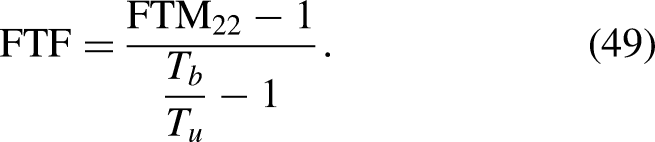
with the burner flame transfer matrix (BFTM) covering acoustics and flame dynamics and the burner transfer matrix (BTM) accounting only for the acoustic transfer functions. Note that the passive flame, that is, the temperature profile is contained in the BTM to isolate the flame response from the acoustics. Subsequently, the FTF is reconstructed according to equation (40) from the ${\mathrm{FTM}}_{22}$ element

$$\mathrm{FTF}=\frac{{\mathrm{FTM}}_{22}-1}{\frac{T_b}{T_u}-1}$$

(49)

In order to emphasize the contribution of the different transfer matrix elements, the transfer matrix ${\mathrm{FTM}}^{+}$ of the non-dimensional effective acoustic pressure and axial velocity ${\hat{p}}_{\mathrm{mn}}^{+}=\frac{{\hat{p}}_{\mathrm{mn}}}{{\rho }_b{c}_b^2}$ and ${\hat{u}}_{\mathrm{mn}}^{+}=\frac{{\hat{u}}_{\mathrm{mn}}}{c_b}$ is used in the following. The diagonal elements ${\mathrm{FTM}}_{11}^{+}={\mathrm{FTM}}_{11}$ and ${\mathrm{FTM}}_{22}^{+}={\mathrm{FTM}}_{22}$ are not effected by the normalisation, since they are non-dimensional already. The contributions of the transfer matrix elements ${\mathrm{FTM}}_{12}^{+}=\frac{{\mathrm{FTM}}_{12}}{{\rho }_b{c}_b}$ and ${\mathrm{FTM}}_{21}^{+}={\mathrm{FTM}}_{21}{\rho }_b{c}_b$ in comparison to the diagonal elements, however, become more clear after normalisation.

Application of the observed flame length of the experiment $L_{\mathrm{Fl}}=10d_T$ to the numerical model leads to a trivial FTM with ${\mathrm{FTM}}_{22}\approx 1$ . Considering the axial integral of Figure 6, the long flame length in relation to the convective wave number yields a high degree of compensation of the heat release fluctuation patches ${\dot{q}}_{\pm }^{\prime }$ in axial direction and thus too low integral gain for a sufficient FTM reconstruction. Higher gain values might be achieved in the experiment by increasing the reactivity of the fuel to achieve shorter flames while keeping the convective wave length constant in the future, which is showcased for a flame length of $L_{\mathrm{Fl}}=3d_T$ in Figure 9 for the reconstructed ${\mathrm{FTM}}^{+}$ obtained from the numerical model.

Figure 9.

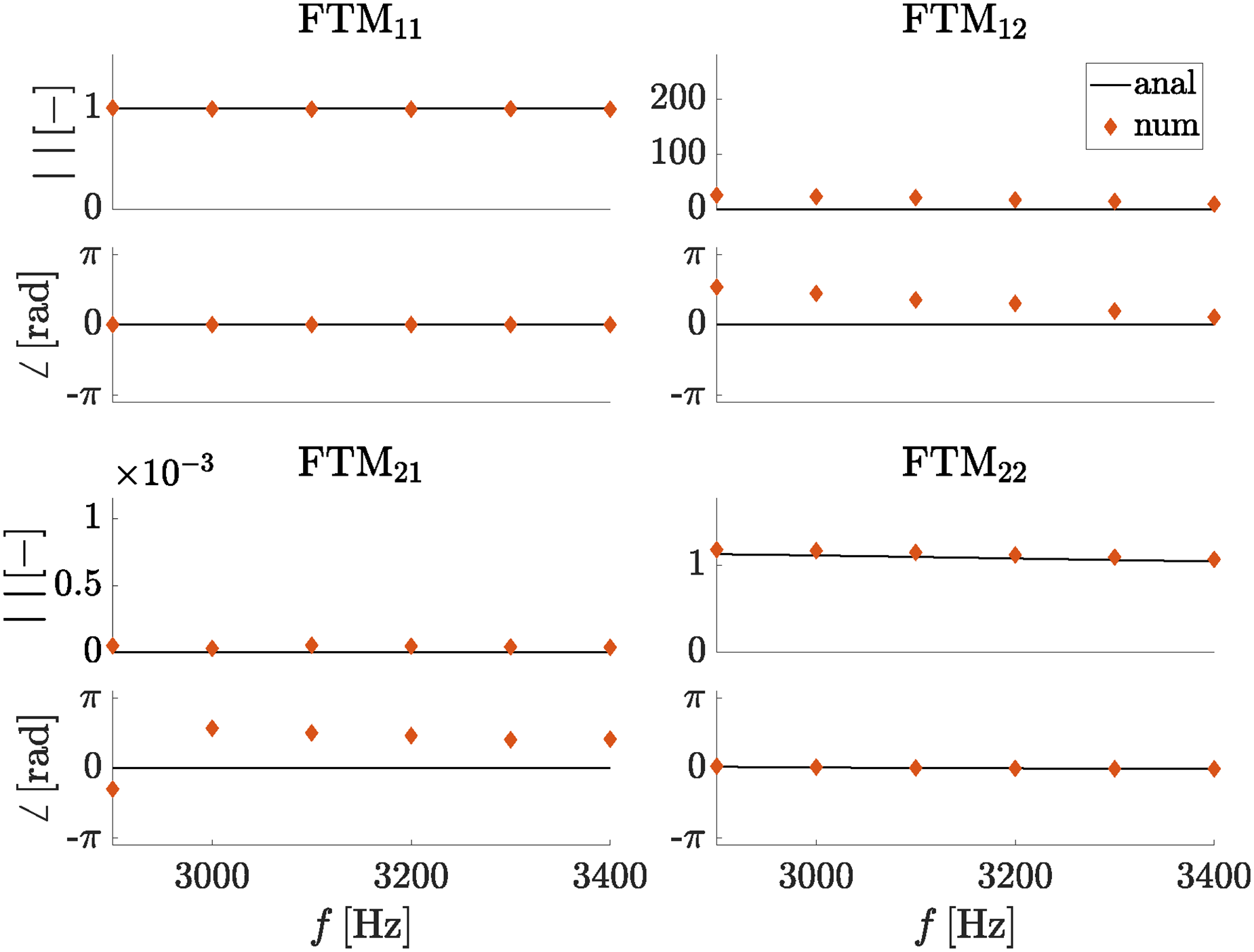
Gain (top) and phase (bottom) of the ${\mathrm{FTM}}_{ij}^{+}$ elements of the numerical MJC model and the analytical model equation (40) for a flame length of $L_{\mathrm{Fl}}=3d_T$ reconstructed with the MMM applied to the effective acoustic pressure and velocity accounting for a passive flame BTM. FTM: flame transfer matrix; MJC: multi-jet combustor; MMM: multi-microphone-method; BTM: burner transfer matrix.

The ${\mathrm{FTM}}_{11}^{+}$ element yields a gain of unity and zero phase as predicted by the model. The elements ${\mathrm{FTM}}_{12}^{+}$ and ${\mathrm{FTM}}_{21}^{+}$ are negligible in comparison to the ${\mathrm{FTM}}_{11}^{+}$ and ${\mathrm{FTM}}_{22}^{+}$ element, since the passive flame is included in the BTM. The depicted flame length of $L_{\mathrm{Fl}}=3d_T$ yields a gain and a phase lag in the ${\mathrm{FTM}}_{22}$ element in exact agreement to the analytical model, which demonstrates the applicability of the transfer matrix method to the HF regime.

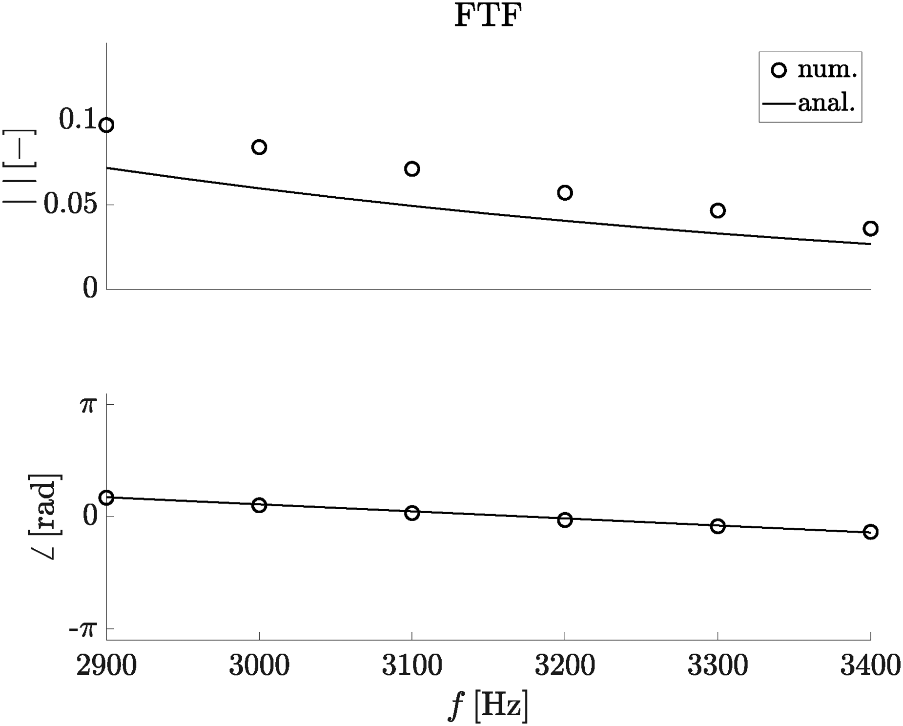
The reconstructed FTF using equation (49) for $L_{\mathrm{Fl}}=3d_T$ is depicted in Figure 10, which shows good agreement with the analytical convective wavenumber model. The predicted gain values of the analytical model deviate to lower values by a constant factor of 0.7 compared to the numerical solution. The observed phase lag is equal to the time delay from the injector tube exit to the ‘centre of gravity’ of the flame close to ${\overline{x}}_{\dot{q}}=L_{\mathrm{Fl}}/2$ obtained from the axial Gaussian distribution. Figure 10 shows moderate to low gain values, since only the flame length is changed in comparison to the experiment. However, the sensitivities of the gain contained in the convective Strouhal number outlines that for the same combustor configuration at the same frequencies, the simple scaling rule $|\mathrm{FTF}|\propto e^{-{\mathrm{St}}^2}$ yield increased gain values with either decreasing frequency and flame length and increased mean flow velocity. Thus, small injector tube diameters and a large combustion chamber diameter (i.e. low cut on frequency $f_{mn}=\frac{{\alpha }_{mn}{\overline{c}}_b}{\pi d_C}$ ) yield high gain values at high frequencies, since the flame length $L_{\mathrm{Fl}}\propto d_T$ becomes similar to the convective wave length ${\lambda }_{\mathrm{conv}}\propto \frac{f_{mn}}{{\overline{u}}_{\mathrm{Fl},x}}$ . For instance, scaling up the plenum and combustor diameter and the radial injector tube position by a factor of 1.5 yields 4 times higher gain values of $0.4-0.2$ in a 1000 Hz lower frequency range, due to the decreased cut on frequency.

Figure 10.

Gain (top) and phase (bottom) of the FTF of the numerical MJC model and the analytical model for a flame length of $L_{\mathrm{Fl}}=3d_T$ reconstructed with the MMM applied to the effective acoustic pressure and velocity accounting for a passive flame BTM. FTF: flame transfer function; MJC: multi-jet combustor; MMM: multi-microphone-method; BTM: burner transfer matrix.

Conclusion

This article provides an extension of the transfer matrix method, as used in LF network models, to the HF regime, providing efficient linear stability tools for gas turbine combustor stability analysis. The conservation equations reveal similar jump conditions across an area change or a flame for the HF regime compared to the LF regime. Two major differences compared to the LF regime are identified. First, the correct control volume to account for in the integral jump conditions across an area change or a flame. Second, the weighting of the amplitudes by means of the effective acoustic area as a consequence of the transverse mode shape. With the theory provided, high frequency burner and flame transfer matrices might be extracted from experiments or CFD, as demonstrated with the numerical model. The theoretical base and validation of a local, HF convective FTF is given with application to numerical CFD/CAA and low-order network models. The experimental results in comparison to the numerical Helmholtz model reveal axial acoustic velocity fluctuations as the predominant cause of the flame response. Further validation of the axial acoustic velocity at the burner mouth is in progress and part of the upcoming PhD thesis of the first author. Additionally, the investigation of equivalence ratio fluctuations to the flame response remains a future task.