Flame transfer function shaping for robust thermoacoustic systems: Application to a kinematic flame model

Abstract

This work presents a data-driven optimization technique for the optimization of the flame response within a low-order acoustic network model. The methodology exploits the Nyquist criterion to compute a measure of thermoacoustic robustness at targeted frequencies, which serves as an objective value for the optimized system. The method is demonstrated using a simple Rijke tube model coupled with a $G$ -equation solver to model flame dynamics. The approach is shown to efficiently increase the stability margin of the system by modifying the flame transfer function. The methodology is applied to two examples, based on which possible scenarios are discussed and the potential and limitations associated with the practical implementation of the method are analyzed.

Introduction

Thermoacoustic oscillations pose a significant problem for gas turbine combustor design. They cause pressure fluctuations with large amplitudes, which limit the safe operating range of the machines and increase the probability of mechanical damage due to fatigue.^1–3

By varying the geometrical and operational parameters of a combustor, optimization methods can be used to identify parameter combinations that minimize the risk of thermoacoustic instability. Adjoint-based methods, which are linear algebra tools that require knowledge of the equations that drive the dynamics of the problem, have been extensively employed in thermoacoustics to assess how changes in operating parameters or geometry affect the thermoacoustic eigenvalues (EVs) and the overall stability of the system.^4–6 These methods can be embedded in classic optimization routines to, for example, ensure that a set of thermoacoustic EVs has a sufficiently large damping rate, as demonstrated by Aguilar and Juniper. ⁴

More recently, purely data-driven optimization methods have received attention in the field of combustor design. These methods do not require knowledge of the underlying physics, but perform a black-box type of optimization by iteratively changing parameters and assessing the improvement. Although some studies report on optimization of steady quantities in combustion,^7–10 optimization involving combustion dynamics poses specific challenges. Consequently, studies on such applications are rare. The experimental application of purely data-driven optimization methods to thermoacoustics was demonstrated by Paschereit et al., ¹¹ who identified fuel injection locations that simultaneously minimize emission levels and thermoacoustic pulsation amplitudes. For optimization, a test rig with adjustable acoustic boundary conditions was used to provide machine-like acoustics. Challenges in incorporating thermoacoustic oscillations into data-driven burner optimization software have recently been addressed in a number of papers, using low-order models. Reumschüssel et al. ¹² compared different optimization methods for optimal positioning of fuel injectors in a low-order model to reduce pressure oscillations from thermoacoustics. Huhn and Magri ¹³ presented a neural network approach for time prediction of chaotic thermoacoustic oscillations to overcome data sparsity and apply data-driven optimization.

One common way to estimate the thermoacoustic stability of a combustion system without an adaptable test rig is to consider the flame response and the engine acoustics separately. In combustion experiments, the flame response to acoustic perturbations is captured by means of acoustic excitation at distinct frequencies. This allows capturing the flame transfer function (FTF), which is the response in heat release rate oscillations of a flame to acoustic perturbations. When combined with a reduced-order model of engine acoustics, thermoacoustic stability can be estimated prior to full engine tests.^11,14 While this approach yields the thermoacoustic spectrum, it has the disadvantage of being costly, due to the large number of experiments required for measuring FTFs. Therefore, incorporating extensive FTF measurements into data-driven optimization is prohibitively expensive. An approach to reduce the experimental cost of optimization was implemented by Bade et al. ¹⁵ In their approach, FTFs were first measured for different operating and geometry parameters and then approximated by parametric models. ¹⁶ In this way, FTFs could be predicted for different parameters so that, by integrating the FTFs into a low-order acoustic model, the parametric dependence of thermoacoustic stability could be predicted, allowing for a data-driven optimization. Although this approach omits the need to remeasure FTFs for each parameter combination considered in the optimization, a database of complete FTFs is still required.

The present study introduces a data-driven optimization method that only requires the measurement of the flame response at some potentially critical frequencies where instabilities are most likely to occur. The resulting small number of required tests at individual frequencies makes the method particularly suitable for experimental testing of real systems. The optimization objective is to maximize the stability margin. The greater the stability margin, the greater the changes to the FTF and the acoustic model can be without the overall system becoming unstable, i.e. the more robust the system. This also enables the application to systems where the description based on the FTF and low-order acoustics is subject to model and measurement errors. Both the stability margin and potentially critical frequencies are identified using the Nyquist stability criterion, a well-known method to evaluate the stability of a thermoacoustic system.^17–19

In the following, we demonstrate the methodology using a simple Rijke tube acoustic model coupled with a $G$ -equation solver to model the flame dynamics.^20,21 The $G$ -equation is a nonlinear kinematic flame model that can be considered realistic as it can resolve complex phenomena such as the formation of cusps and pinch-offs ²² and nonlinear thermoacoustic coupling. ²³ In addition, the model enables the consideration of hydrodynamic fluctuations as well as fluctuations in the equivalence ratio. ²⁴ Two parameters of the flame model are used as degrees of freedom for the optimization routine. They represent possible changes to the combustion chamber that affect the flame response to acoustic perturbations. It is assumed that the combustion chamber acoustics are not affected by parameter changes. Accordingly, the goal of the optimization is to shape the FTF in such a way that the thermoacoustic system is as robust as possible.

As is common for experiments, the flame response is obtained by acoustic forcing at distinct frequencies with low amplitude and measuring the heat release fluctuations. ²⁵ This study is a continuation of our previous paper, ²⁶ in which the robust combustor design approach was presented theoretically. In the present study, we apply the method to a realistic thermoacoustic model.

This manuscript is structured as follows. We first describe the low-order model for the acoustics in the combustor and the $G$ -equation framework for simulation of the flame response. This is followed by a short introduction to the Nyquist stability criterion, from which equations for the stability margin and critical frequencies are derived. These are used in the subsequently described optimization algorithm. The method is finally applied to different cases, based on which possible scenarios are discussed and the potential and limitations of the methodology are analyzed.

Thermoacoustic model

In order to experimentally characterize the thermoacoustics of a gas turbine burner, both the flame response and the acoustic boundary conditions must be adapted to the conditions in the machine, which involves significant effort.^27,28 Resolving the interaction between acoustics, hydrodynamics and flame dynamics numerically in high-fidelity simulations is also very costly. With today’s computing power, single high-resolution simulations can be performed, but the associated costs are generally prohibitive for extensive design studies considering different operating conditions. ³ Therefore, network analyses or finite element calculations remain the most efficient and common approaches to investigate thermoacoustic stability.^29,30 The involved acoustics and flame dynamics are first analyzed independently and then integrated into a feedback loop via first principle approaches. In this study, the concept of robust combustor design optimization will be demonstrated by using one-dimensional acoustics and a conical flame, as introduced in the following.

Acoustic model

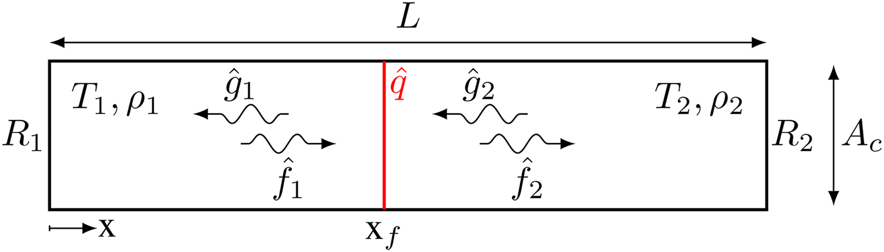
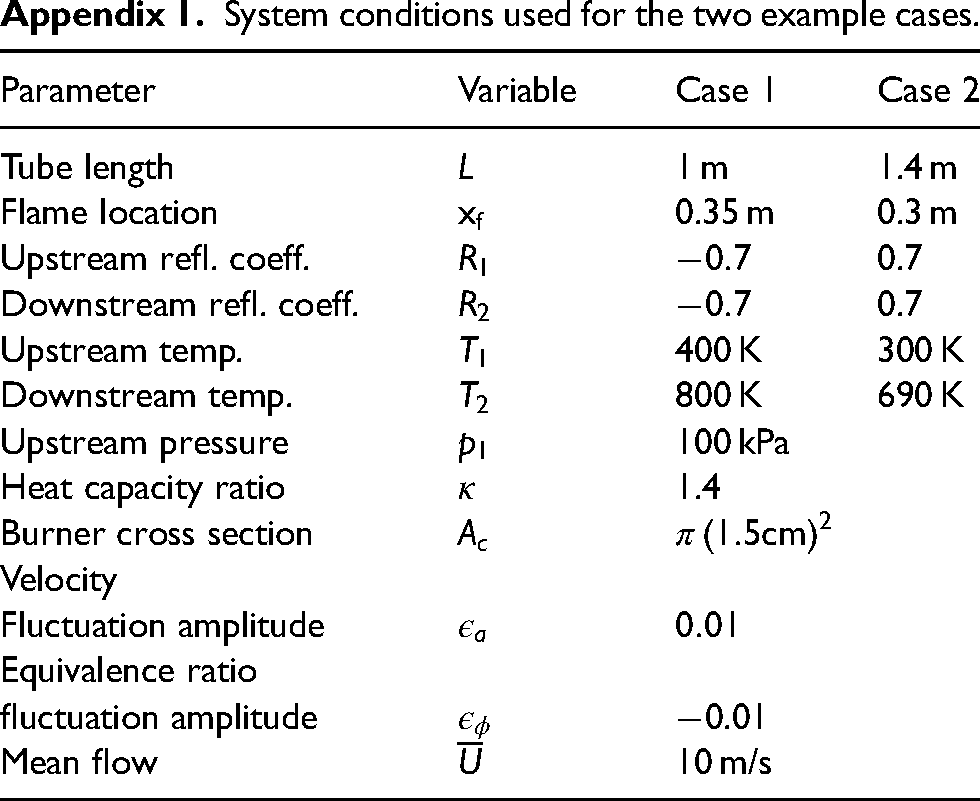
As in our previous study, we consider a generic example and model the combustion chamber as a Rijke tube, ²⁶ depicted in Figure 1. In the following, we briefly outline how plane acoustic waves in a Rijke tube can be modelled. ²⁹ The length of the tube is referred to as $L$ . At ${\text{x}}_f$ the flame separates the combustor into a cold ( $T_1$ ) upstream and a hot ( $T_2$ ) downstream region. Note that we vary some of the acoustic quantities to create different cases. The corresponding values are therefore listed in the results section.

Figure 1.

Sketch of a generic combustion chamber modelled as a Rijke tube.

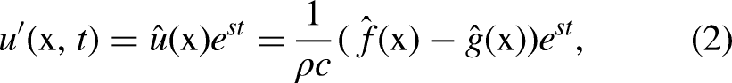
Planar acoustic waves propagate in both regions so that the acoustic pressure and velocity can be expressed by

$$p^{\prime }(\text{x},t)=\hat{p}(\text{x})e^{st}=(\hat{f}(\text{x})+\hat{g}(\text{x}))e^{st},$$

(1)

$$u^{\prime }(\text{x},t)=\hat{u}(\text{x})e^{st}=\frac{1}{\rho c}(\hat{f}(\text{x})-\hat{g}(\text{x}))e^{st},$$

(2)

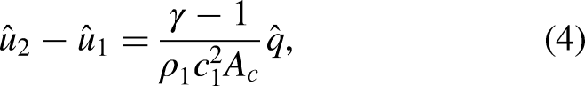
where $\hat{f}(\text{x})=\mathit{f}{e}^{-\frac{\text{x}s}{c}}$ and $\hat{g}(\text{x})={\mathit{g}\mathit{e}}^{+\frac{\text{x}s}{c}}$ are the up- and downstream travelling acoustic waves with complex amplitudes $f$ and $g$ . The speed of sound is denoted as $c$ , the mean gas density as $\rho$ and the complex-valued frequency as $s=\sigma +i\omega$ , where $i$ is the imaginary unit. At the up- and down stream ends of the duct, the acoustic waves are reflected with reflection coefficients $R_1$ and $R_2$ , respectively. Across the compact flame element, the Rankine-Hugoniot jump conditions are applied

$${\hat{p}}_2-{\hat{p}}_1=0,$$

(3)

$${\hat{u}}_2-{\hat{u}}_1=\frac{\gamma -1}{{\rho }_1{c}_1^2{A}_c}\hat{q},$$

(4)

where $\hat{q}$ denotes the complex amplitude of the heat release oscillation. The two boundary conditions (up- and down-stream reflection) together with the two jump conditions can be expressed in the following form.

$$\mathbf{M}(s)\mathbf{g}=\mathbf{q},$$

(5)

where $\mathbf{g}$ contains the amplitudes of the acoustic waves $f$ and $g$ in the up- and down stream region and $\mathbf{M}$ is called the acoustic matrix in the following. Without heat release oscillations ( $\mathbf{q}=\mathbf{0}$ ) the acoustic EVs can be computed by solving $\text{det}[\mathbf{M}(s)]=0$ . If a flame transfer function is given, $\mathbf{q}$ can be expressed as a function of $\mathbf{g}$ . Then, the heat release term can be incorporated in the acoustic matrix such that ${\mathbf{M}}_f(s)\mathbf{g}=\mathbf{0}$ and the thermoacoustic EVs can be determined. In the scope of this study all thermoacoustic EVs are computed in this way, i.e. by solving $\text{det}[{\mathbf{M}}_{\mathit{f}}(s)]=0$ .

Alternatively, by inverting the acoustic matrix the response of the acoustics to heat release fluctuations can be computed by first solving Equation (5) for the amplitudes of the acoustic waves $\mathbf{g}$ , and then substituting the result in Equations (1) and (2) to compute the acoustic pressure and velocity. The transfer function that relates velocity fluctuations upstream of the flame to heat release fluctuations is denoted acoustic transfer function (ATF) in the following.

Kinematic flame model

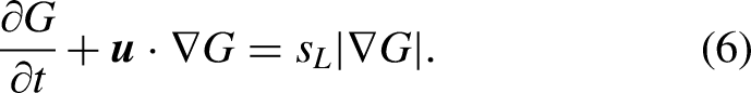
To simulate the flame response to acoustic excitation we model the dynamics of an axisymmetric conical flame subject to equivalence ratio fluctuations by using the kinematic $G$ -equation, which reads ³¹

$$\frac{\mathrm{\partial }G}{\mathrm{\partial }t}+\mathit{u}\cdot \mathrm{\nabla }G=s_L|\mathrm{\nabla }G|.$$

(6)

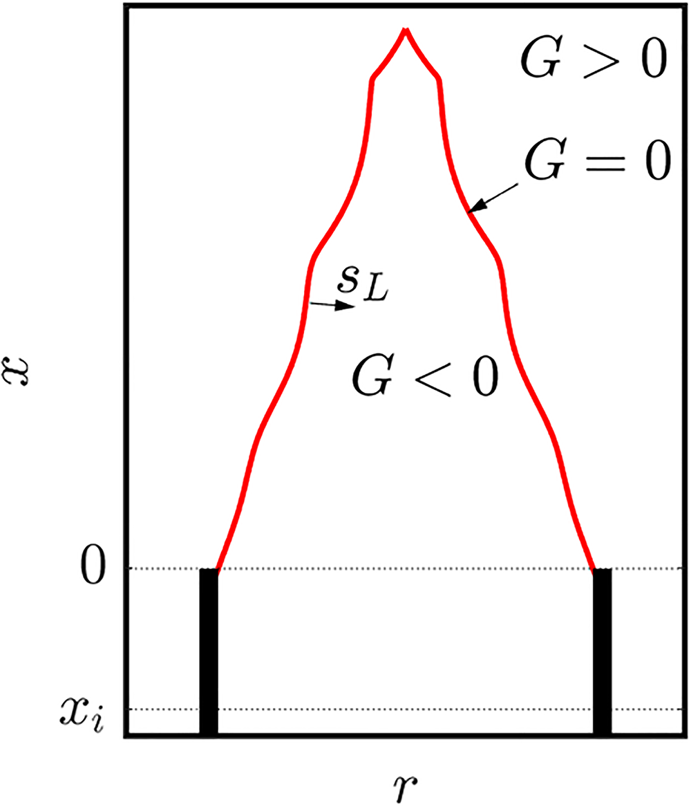
Here, $G=G(x,r,t)$ denotes a scalar field that takes negative values in the unburned gas region, positive values in the burned gas region, and zero at the flame front. Figure 2 shows a sketch of the $G$ -field. Note that in the acoustic model, the flame is modelled as a discontinuity at location $\text{x}={\text{x}}_f$ while the flame response is modelled in a two-dimensional field with normalized cylindrical coordinates $x$ and $r$ . $s_L=s_L(x,r,t)$ denotes the local flame speed, which is a function of the local equivalence ratio $\varphi =\varphi (x,r,t)$ and follows the empirical relation ³²

$$s_L=A{\varphi }^B{e}^{-C(\varphi -D{)}^2},$$

(7)

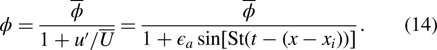
where $A$ =0.6079, $B$ =-2.554, $C$ =7.31, and $D$ =1.230 are empirical constants. The velocity vector field $\mathit{u}=\mathit{u}(x,r,t)$ has an axial component $u=u(x,t)$ and a radial component $v=v(x,r,t)$ . The axial velocity is prescribed to have the form

$$u/\overline{U}=1+{ϵ}_a\sin \left[\mathrm{St}(t-Kx)\right],x\ge 0,$$

(8)

where $\overline{U}$ is the mean bulk velocity, $\mathrm{St}$ the Strouhal number, $K$ a non-dimensional convective speed and ${ϵ}_a$ the amplitude of the unsteady velocity fluctuations $u^{\prime }/\overline{U}$ . In the radial direction, the mean flow field is assumed to be zero, and the unsteady fluctuations $v^{\prime }$ are determined by imposing mass conservation for an incompressible flow. This velocity model has been widely employed in the literature^33,34 and models the formation and roll up of vortical structures along the flame shear layer. In the burner domain ( $x<0$ ), instead, no vortex modulation is considered and the flow is assumed to undergo incompressible oscillations with

$$u/\overline{U}=1+{ϵ}_a\sin \left(\mathrm{St}t\right),x<0.$$

(9)

The equivalence ratio is modulated at the injector location $x_i<0$ and is assumed to be transported by the (uniform) mean flow only. The $\varphi$ field reads

$$\varphi /\overline{\varphi }=1+{ϵ}_{\varphi }\sin \left[\mathrm{St}(t-(x-x_i))\right],$$

(10)

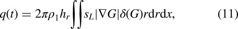
where $\overline{\varphi }$ denotes the mean equivalence ratio, $x_i$ is the normalized location of fuel injection and ${ϵ}_{\varphi }$ the amplitude of equivalence ratio fluctuations ${\varphi }^{\prime }/\overline{\varphi }$ . The unsteady heat release can be computed from an integration across the flame surface over the computational domain

$$q(t)=2\pi {\rho }_1{h}_r\int \int s_L|\mathrm{\nabla }G|\delta (G)r\text{d}r\text{d}x,$$

(11)

where $h_r$ is the reaction enthalpy and $\delta$ denotes the Dirac function.

Figure 2.

Sketch of the kinematic model for the flame front evolution based on the $G$ -equation.

Stiff injector model

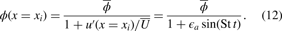
The amplitudes of the acoustic velocity and equivalence ratio fluctuations are not necessarily independent. For an ideal injector at location $x=x_i$ , for which the fuel injection is unaffected by the acoustic perturbations in the air flow, ³⁵ the following nonlinear relation between the equivalence ratio and the axial velocity fluctuations holds:

$$\varphi (x=x_i)=\frac{\overline{\varphi }}{1+u^{\prime }(x=x_i)/\overline{U}}=\frac{\overline{\varphi }}{1+{ϵ}_a\sin \left(\mathrm{St}t\right)}.$$

(12)

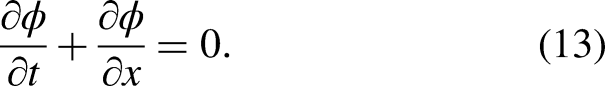
This equation acts as a boundary condition for the advection equation that governs the transport of the equivalence ratio:

$$\frac{\mathrm{\partial }\varphi }{\mathrm{\partial }t}+\frac{\mathrm{\partial }\varphi }{\mathrm{\partial }x}=0.$$

(13)

Note that $x$ and $t$ were normalized with $\overline{U}$ such that the advection speed is one here. Diffusion effects are neglected in this study but could be included. ³⁶ Equation (13) with the boundary condition Equation (12) can be solved to yield an explicit expression for the equivalence ratio field:

$$\varphi =\frac{\overline{\varphi }}{1+u^{\prime }/\overline{U}}=\frac{\overline{\varphi }}{1+{ϵ}_a\sin \left[\mathrm{St}(t-(x-x_i))\right]}.$$

(14)

By expanding this equation to first order for small oscillation amplitude ${ϵ}_a$ , one obtains

$$\varphi /\overline{\varphi }=1-{ϵ}_a\sin \left[\mathrm{St}(t-(x-x_i))\right].$$

(15)

By comparing this equation with Equation (10) we obtain that for the stiff injector model to hold, we must impose ${ϵ}_{\varphi }=-{ϵ}_a$ . In the present study ${ϵ}_{\varphi }$ and ${ϵ}_a$ are fixed to $-0.01$ and $0.01$ , respectively. The remaining two parameters of the flame model, injector location $x_i$ and convection speed $K$ , serve as degrees of freedom for optimization.

Flame frequency response

The flame response is characterized by the flame transfer function, which relates the unsteady heat release to fluctuations in velocity. To obtain the FTF, the $G$ -equation framework is used for time series simulations of the flame response at distinct forcing frequencies, as is it commonly done in experimental measurements. Therefore, the Strouhal number is adjusted according to the forcing frequency and the simulation is carried out for $5$ oscillation periods. The heat release is then captured (Equation (11)) and related to the acoustic velocity fluctuations at the flame base ( $x=0$ ) to obtain the frequency response of the flame.

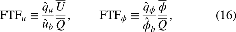
Although the proposed optimization routine is purely data-driven and does not use any physical knowledge, we will briefly consider the influence of the two physical mechanisms affecting the FTF in the following. Because the FTF is a linear quantity, the contribution from the formation of fluctuations of the equivalence ratio, FTF _ϕ , can be separated from the contribution due to velocity fluctuations, FTF _u . In experiments, this separation is not always easy to achieve because the two effects may be coupled.^35,37 Numerically, however, we can turn each effect on and off at will. We define FTF _u and FTF _ϕ , respectively, as

$${\text{FTF}}_u\equiv \frac{{\hat{q}}_u}{{\hat{u}}_b}\frac{\overline{U}}{\overline{Q}},{\text{FTF}}_{\varphi }\equiv \frac{{\hat{q}}_{\varphi }}{{\hat{\varphi }}_b}\frac{\overline{\varphi }}{\overline{Q}},$$

(16)

where the hats denote Fourier transforms. The reference signals used to define FTF _u and FTF _ϕ are the fluctuations in the velocity and equivalence ratio at the base of the flame ( $x=0$ ), respectively. They read

$$u_b^{\prime }=u^{\prime }(x=0)={ϵ}_a\overline{U}\sin \left(\mathrm{St}t\right),$$

(17)

$${\varphi }_b^{\prime }={\varphi }^{\prime }(x=0)={ϵ}_{\varphi }\overline{\varphi }\sin \left[\mathrm{St}(t+x_i)\right].$$

(18)

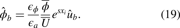
In the frequency domain, the reference signals are related by

$${\hat{\varphi }}_b=\frac{{ϵ}_{\varphi }}{{ϵ}_a}\frac{\overline{\varphi }}{\overline{U}}{e}^{s{x}_i}{\hat{u}}_b.$$

(19)

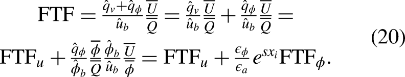
When both velocity and equivalence ratio fluctuations are present, it is typical to scale the total FTF by using a reference velocity signal only. Linear superposition yields the following relation between the total FTF and the partial contributions of FTF _ϕ and FTF _v .

$$\begin{array}{cc}& \text{FTF}=\frac{{\hat{q}}_v+{\hat{q}}_{\varphi }}{{\hat{u}}_b}\frac{\overline{U}}{\overline{Q}}=\frac{{\hat{q}}_v}{{\hat{u}}_b}\frac{\overline{U}}{\overline{Q}}+\frac{{\hat{q}}_{\varphi }}{{\hat{u}}_b}\frac{\overline{U}}{\overline{Q}}=\\ & {\text{FTF}}_u+\frac{{\hat{q}}_{\varphi }}{{\hat{\varphi }}_b}\frac{\overline{\varphi }}{\overline{Q}}\frac{{\hat{\varphi }}_b}{{\hat{u}}_b}\frac{\overline{U}}{\overline{\varphi }}={\text{FTF}}_u+\frac{{ϵ}_{\varphi }}{{ϵ}_a}{e}^{s{x}_i}{\text{FTF}}_{\varphi }.\end{array}$$

(20)

In the last step the FTF _ϕ definition, Equation (16), and the relation in Equation (19) were used. Note that this model is causal, because $x_i$ is negative.

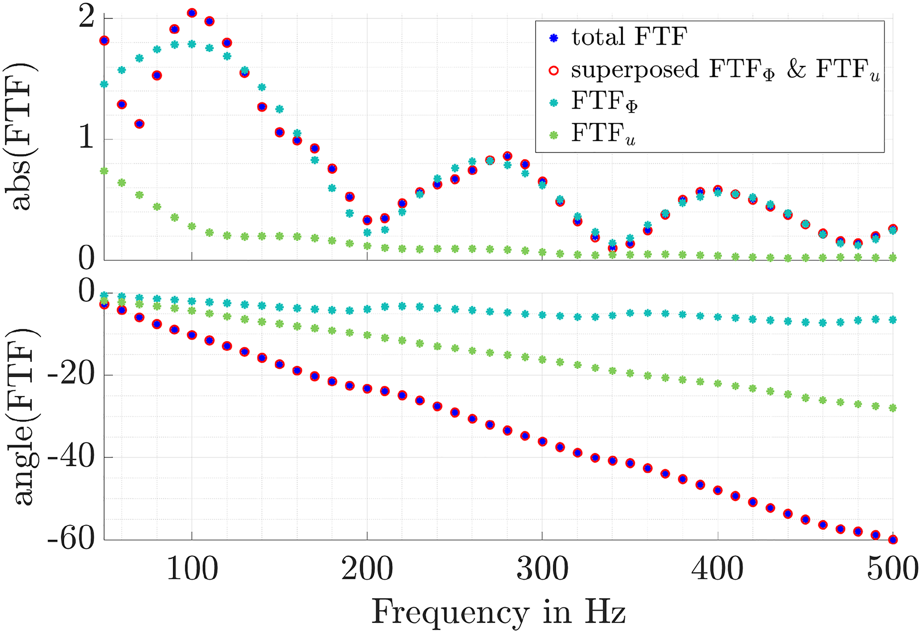
Figure 3 shows the two FTF contributions (green and light blue) for an exemplary configuration. The total FTF is the result of superposition according to Equation (20). It can be calculated by switching on both effects in the $G$ -equation system and is shown in dark blue in Figure 3. To validate the framework, we ensured that this is identical to the superposition of the individually simulated FTF contributions according to Equation (20) (see Figure 3).

Figure 3.

Flame transfer function (FTF) contribution from velocity fluctuations ( ${\text{FTF}}_u$ , green markers) and from equivalence ratio fluctuations ( ${\text{FTF}}_{\varphi }$ , light blue markers). Dark blue markers show total $\text{FTF}$ and red circles show superposition of individually simulated FTF contributions (Equation (20)).

For the shown case, the gain of the total FTF is mainly influenced by fluctuations in the equivalence ratio. The contribution of ${\text{FTF}}_u$ is only significant for frequencies below 200 Hz. However, due to interaction of the two effects in the low-frequency range, constructive and destructive interactions occur, resulting in a more complex shaped gain curve. The occurrence of such a dominant mechanism that is superposed by others is also found in experimental work and can thus be considered realistic. ³⁸

The decomposition of the FTF highlights the influence of the optimization parameters, $x_i$ and $K$ on the flame response. The injection location $x_i$ affects the relative phase between the flame response to velocity fluctuations and the response to $\varphi$ fluctuations. The convection speed $K$ modifies the FTF contribution from velocity fluctuations, without altering the part due to equivalence ratio fluctuations. Such a variation in transport speed of velocity fluctuations could, for example, be generated in a real combustor by small geometric variations such as the installation of an obstacle upstream of the flame. ³⁹

Stability assessment using the Nyquist stability criterion

In this section, we briefly introduce the Nyquist stability criterion for feedback systems which is commonly used in control engineering.^40,41 By applying it to thermoacoustics, quantities are derived that are used for data-driven robust combustor optimization.

Thermoacoustics as a feedback loop

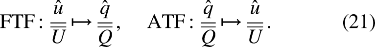
Thermoacoustic oscillation occur as a result of acoustically driven heat release fluctuations which in turn generate acoustic oscillations. ²⁹ Separating acoustics and the flame response yields the following definitions for the flame and acoustic transfer functions:

$$\text{FTF}:\frac{\hat{u}}{\overline{U}}\mapsto \frac{\hat{q}}{\overline{Q}},\text{ATF}:\frac{\hat{q}}{\overline{Q}}\mapsto \frac{\hat{u}}{\overline{U}}.$$

(21)

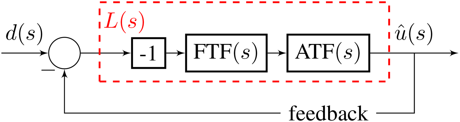
By adopting a perspective from control engineering, the thermoacoustic system can be interpreted as an open loop system, defined as

$$L(s)=-\text{FTF}(s)\text{ATF}(s)$$

(22)

and a feedback loop as depicted in Figure 4. The negative sign is included to be consistent with common control notation.

Figure 4.

Interpretation of a thermoacoustic system as a feedback loop with open loop system $L(s)$ . The open loop system combines the flame and acoustic transfer functions. $d(s)$ is a disturbance and $\hat{u}(s)$ are acoustic velocity oscillations.

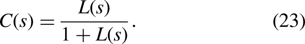
The closed system $C(s)$ describes the transfer of a disturbance $d(s)$ to an acoustic oscillation $\hat{u}(s)$ and includes the feedback. The corresponding closed-loop transfer function reads

$$C(s)=\frac{L(s)}{1+L(s)}.$$

(23)

Open loop-based stability analysis

A common approach to analyse how disturbances are amplified or dampened, i.e. to assess thermoacoustic stability, is to compute the EVs of the closed feedback system. In practice, this requires analytical forms for both acoustics and flame response. ⁴² For this purpose the FTF is usually approximated by an analytical function that requires sampling points at several frequencies. ⁴³ An EV-based optimization of the FTF would therefore be very cost-intensive. Within our routine, we circumvent this obstacle by using the Nyquist stability criterion, which allows evaluation at individual frequencies. However, we also perform EV analyses to discuss our approach. Therefore, the FTF is simulated at frequencies 10 Hz apart in the frequency range 50–500 Hz, resulting in 46 discrete frequency response values. The vector fitting method of Gustavsen and Semlyen ⁴⁴ is then used to obtain a rational representation.

To assess stability from the open loop transfer function (OLTF) directly, the Nyquist stability criterion can be used. ⁴⁰ In the context of thermoacoustics, the Nyquist stability criterion has been used by Polifke et al. ¹⁷ and Richards et al., ¹⁸ among others. Therefore, the mapping $s\to L(s)$ is further analysed. Stability of $C(s)$ is governed by its poles (EVs), $s_{\text{e}}$ , which are the zeros of the denominator of Equation (23). Thus, $L(s)$ maps all the thermoacoustic EVs to $-1$ , which is referred to as the critical point. Furthermore, the so-called Nyquist curve is obtained by mapping the stability line, i.e., the imaginary axis $i\omega$ using the OLTF, $L(i\omega )$ . Because $L(s)$ preserves handedness, the closed loop system is stable if the critical point is on the left-hand side, when following the Nyquist curve from low to high frequencies. ^a

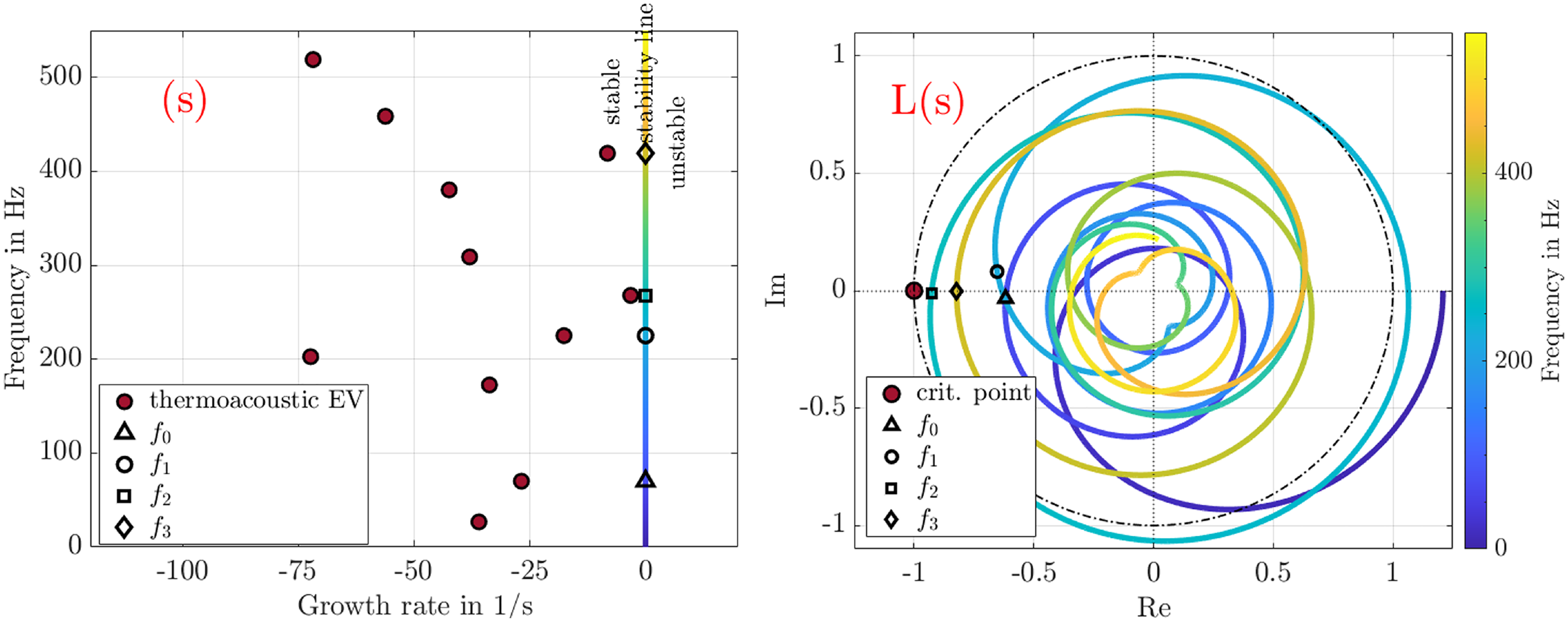
The open loop-based stability analysis is illustrated in Figure 5. The left panel shows the EVs in the complex plane for a thermoacoustic closed-loop system computed with the determinant method explained above. The right panel shows the corresponding $L(s)$ -plane with the Nyquist curve, i.e. the mapped stability line, which is coloured according to frequency. Both stability diagrams indicate a stable system. According to the complex plane, in which all EVs lie to the left of the stability line, the critical point also lies to the left of the Nyquist curve. It can also be seen that the Nyquist curve passes near the critical point once for each EV.

Figure 5.

The Nyquist curve for stability estimation. Left panel: Complex plane $s$ showing the system eigenvalues and the stability line. Right panel: Output of the complex-mapping $L(s)$ . The stability line is mapped to the Nyquist curve (coloured line). The eigenvalues are mapped to the critical point, $-$ 1.

Stability margin and robustness

In Figure 5 the frequencies of the four EVs with the highest growth rate, thus with the greatest proximity to instability, are marked with symbols on the stability line and on the Nyquist curve. It is apparent that the proximity to the critical point can serve as a measure of the risk of instability. The minimal distance to the critical point across all frequencies determines the stability margin $\mu$ . The stability margin can be calculated from the OLTF as

$$\mu =\underset{\omega }{\text{min}}|1+L(i\omega )|.$$

(24)

The higher this distance, the more deviations in gain and phase of ATF and FTF can be tolerated without the closed-loop thermoacoustic system becoming unstable. In control engineering, this system property is termed robustness. To employ the stability measure in an optimization routine for minimization, the so-called sensitivity function $S$ is introduced

$$S(\omega )=\frac{1}{|1+L(i\omega )|}.$$

(25)

The sensitivity function is the inverse of the distance to the critical point and therefore peaks at the most critical frequencies (as shown in Figure 7, for example). In general, the maximum sensitivity and the largest growth rate across the eigenvalues are both valid measures to assess the robustness of a system. However, the Nyquist view allows us to evaluate the sensitivity for single frequencies, while functions are generally necessary for EV calculation. Taking a practical perspective, this allows us to efficiently employ optimization in an experimental framework, where mono-frequent forcing is the common working principle for flame response measurements. Critical frequencies can be identified using the Nyquist curve, for which the sensitivity is then minimized in a data-driven routine. In the following, details about the implementation of this routine are outlined.

Optimization methodology

The objective of the data-driven optimization is to increase the stability margin and thus the robustness of the thermoacoustic system by modifying the flame response. To keep the effort as low as possible, the flame response is only evaluated at potentially critical frequencies, ${\mathrm{\Omega }}_{\text{,pc}}=[{\omega }_{\text{,pc1}},{\omega }_{\text{,pc2}},..]$ . For this purpose, a list of potentially critical frequencies is first initiated using the critical frequency from the initial system, i.e. the frequency at which the sensitivity is maximal,

$${\omega }_{\text{crit}}=\text{argmax}S(\omega ).$$

(26)

To determine this critical frequency, the FTF and ATF must thus be known in the frequency band of interest. After the critical frequency is identified, a data-driven optimization routine is applied to minimize the sensitivity at this critical frequency by modifying the flame response by varying the optimization variables, $K$ and $x_i$ . The well-established exploitive downhill simplex method (DSM) proposed by Nelder and Mead ⁴⁵ is used for this purpose. It compares values of the objective function for $P+1$ combinations of inputs to iteratively find local minima, $P$ being the number of parameters to optimize.

By limiting the iterations of the DSM routine, we prevent detailed, small-scale search steps. Instead, the entire flame transfer function is measured again after $N_{\text{DSM}}=30$ function calls from DSM. Remeasuring the entire flame transfer function after some iterations steps is costly, but a crucial step to consider the stability of the overall system. The remeasured FTF is first used to test whether the system is stable by checking if $\text{Re}(L(s))>-1$ is satisfied for all frequencies. If the parameter set found by the DSM routine leads to a stable full system, we test whether (a) the stability margin has increased and (b) which frequency now exhibits the highest sensitivity. If the critical frequency has shifted significantly (more than 10 Hz), the new value is included in the list of potentially critical frequencies ${\mathrm{\Omega }}_{\text{,pc}}$ . For smaller changes, the old value is replaced. For unstable configurations, the frequency with the smallest associated real part of $L(s)$ is added to ${\mathrm{\Omega }}_{\text{,pc}}$ . Consequently, the number of potentially critical frequencies contained in ${\mathrm{\Omega }}_{\text{,pc}}$ increases in the course of optimization. Once a new ${\omega }_{\text{,pc}}$ is identified, the DSM algorithm is restarted, using the configuration of $K$ and $x_i$ with the highest stability margin $\mu$ as initial values. If ${\mathrm{\Omega }}_{\text{,pc}}$ contains more than one critical frequency, the objective function $J$ is formed by the maximum sensitivity of all potentially critical frequencies in ${\mathrm{\Omega }}_{\text{,pc}}$ ,

$$J(K,x_i)=\underset{\omega \in {\mathrm{\Omega }}_{\text{,pc}}}{\text{min}}S(K,x_i,\omega ).$$

(27)

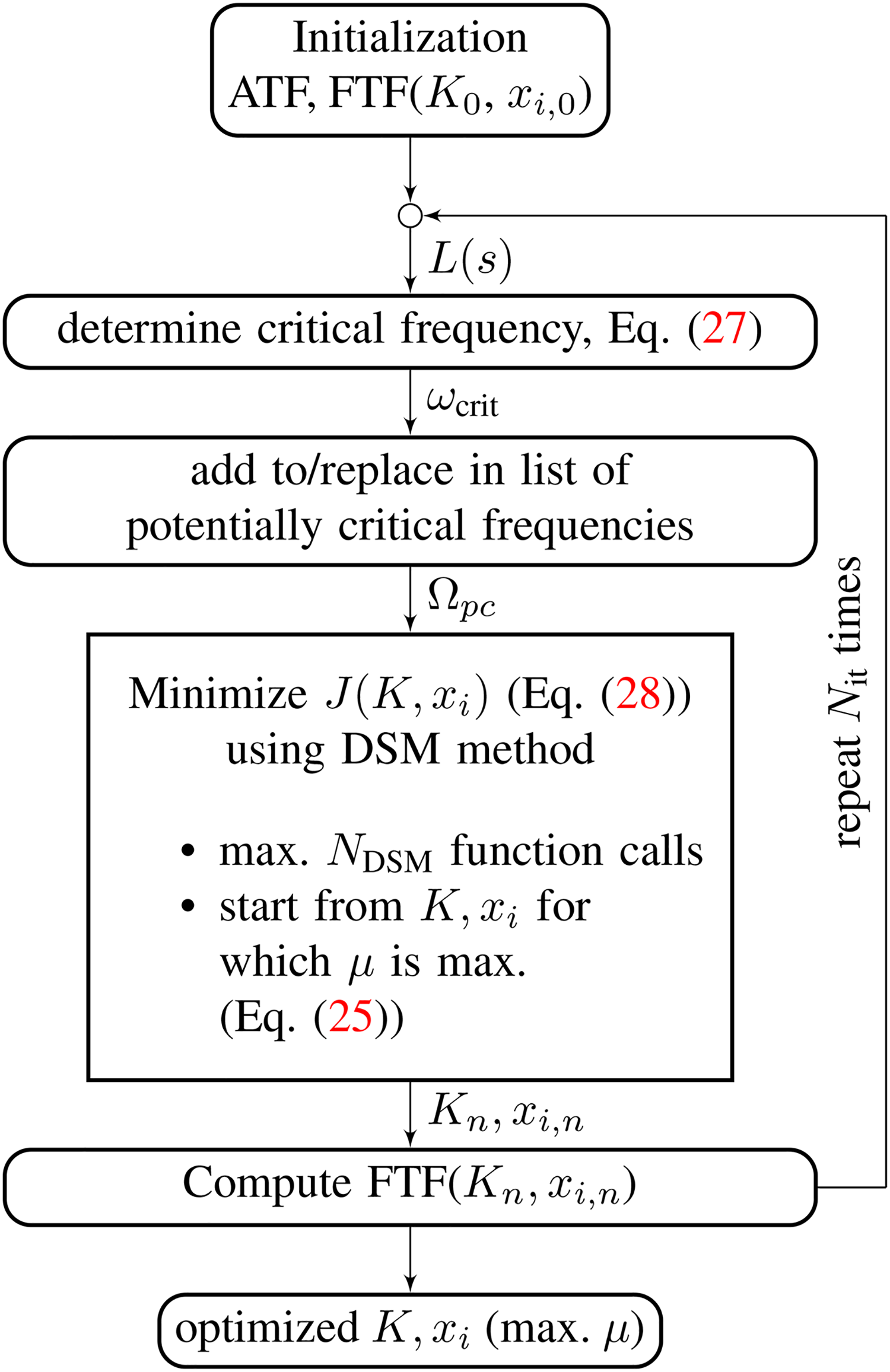
The cost of the optimization increases with the length of ${\mathrm{\Omega }}_{\text{,pc}}$ since for each parameter combination the sensitivity and thus the flame response at all potentially critical frequencies needs to be evaluated. However, expanding the list ensures that the optimizer considers different frequency ranges in which instabilities might occur. To prevent configurations that lead to a destabilization of the system, the cost value is increased by ${10}^4$ within $J$ as soon as the real part of the OLTF $L(s)$ reaches a value smaller than -1 for any of the frequencies included in ${\mathrm{\Omega }}_{\text{,pc}}$ . Although this threshold is not a sufficient criterion for instability, it is highly likely to indicate it. ¹⁹ The top-level routine is repeated $N_{\text{it}}$ times. Thus, a full FTF is calculated $N_{\text{it}}$ times. The method is illustrated in Figure 6.

Figure 6.

Flowchart of the optimization routine.

Results

In the following, the presented optimization routine is applied to the thermoacoustic simulation framework consisting of the $G$ -equation solver and the acoustic network model described above. To generate different scenarios some of the system parameters are changed. Two cases are considered as examples to illustrate the working principle of the algorithm. The corresponding parameter values are listed in Appendix 1. In both cases, the optimization starts at the same flame transfer function, characterized by the initial optimization parameters $K_0=1.2$ and $x_{i,0}=-2$ . The corresponding starting FTF is also shown in Figure 3.

Example Case 1

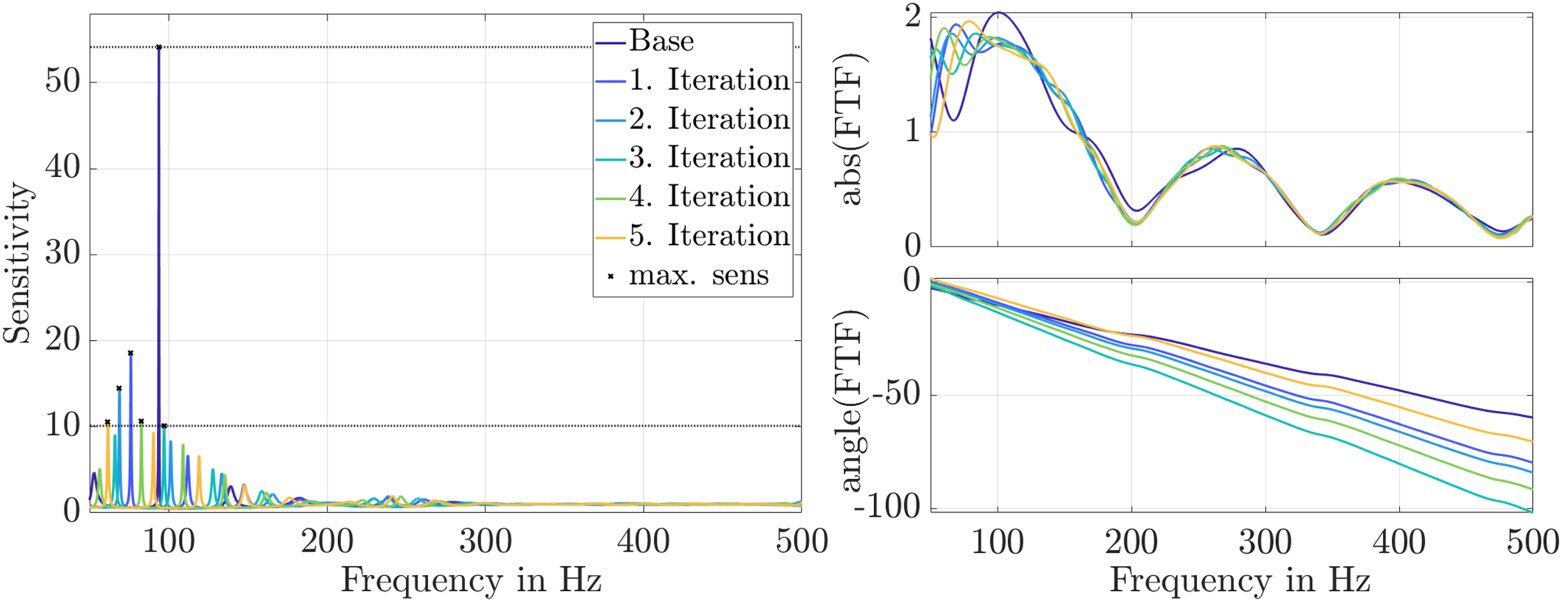
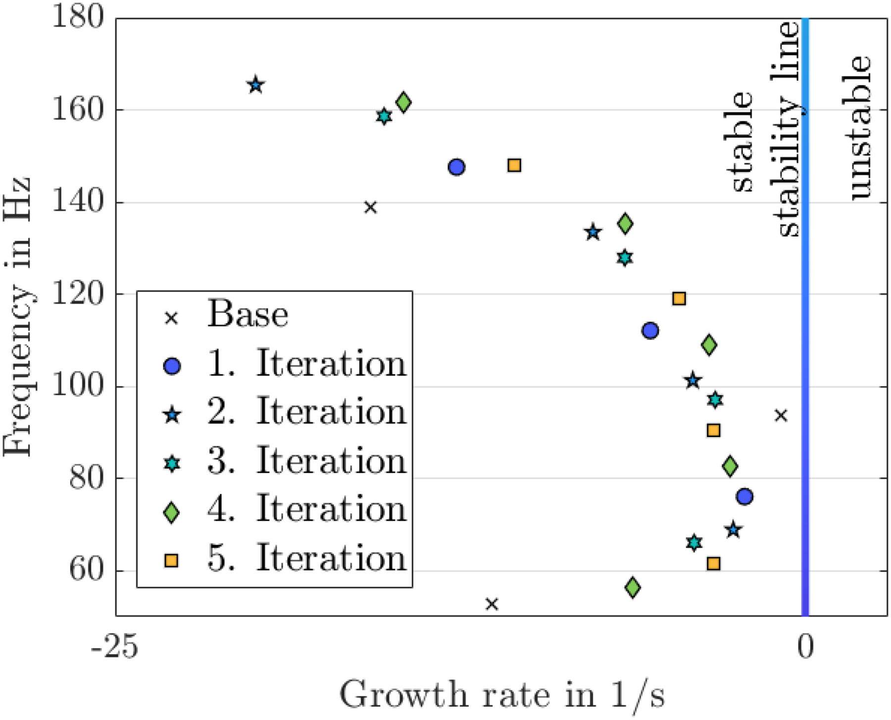
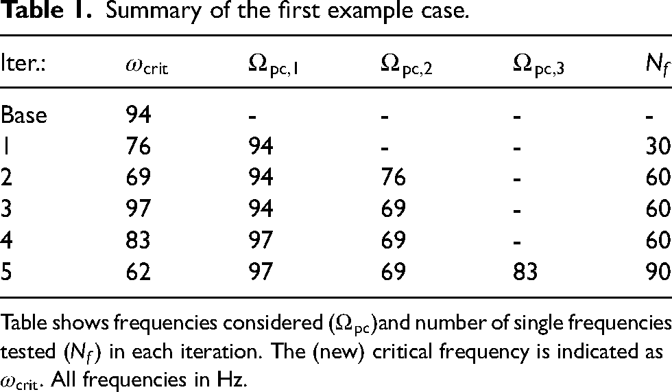
The curves labelled ’Base’ in Figure 7 show the initial FTF and corresponding sensitivity function computed from Equation (25) in the right and left panel, respectively. It can be observed that the thermoacoustic system features a very high sensitivity at $94$  Hz. Accordingly, the Nyquist curve is close to the critical point at this frequency, which is equivalent to an EV close to the stability line, as shown in Figure 8. Starting from this configuration with high sensitivity the optimizer is run for $N_{\mathrm{it}}=5$ iterations. Figure 7 shows the sensitivity curves and FTFs after each iteration in the left and right panel, respectively. The corresponding eigenvalues in the vicinity of the stability line are shown in Figure 8. The list of critical frequencies in each iteration is shown in Table 1.

Figure 7.

Left: Sensitivities of the thermoacoustic system after each iteration of the optimization routine for Case 1. The horizontal dotted lines mark the maximal value of the starting configuration, as well as the smallest maximum found during optimization. Right: Gain and phase of the corresponding flame transfer functions (FTFs).

Figure 8.

Thermoacoustic eigenvalues after each iteration of Case 1.

Table 1.

Summary of the first example case.

Iter.:	${\omega }_{\text{crit}}$	${\mathrm{\Omega }}_{\text{,pc},1}$	${\mathrm{\Omega }}_{\text{,pc},2}$	${\mathrm{\Omega }}_{\text{,pc},3}$	$N_f$
Base	94	-	-	-	-
1	76	94	-	-	30
2	69	94	76	-	60
3	97	94	69	-	60
4	83	97	69	-	60
5	62	97	69	83	90

Table shows frequencies considered ( ${\mathrm{\Omega }}_{\text{,pc}}$ )and number of single frequencies tested ( $N_f$ ) in each iteration. The (new) critical frequency is indicated as ${\omega }_{\text{crit}}$ . All frequencies in Hz.

In the first iteration, the DSM routine shapes the FTF considering the initial critical frequency only, which substantially increases the stability margin. After the first optimization iteration $76$  Hz is identified as the new critical frequency. The optimizer continues shaping the FTF, now taking into account two potentially critical frequencies. After optimizing both frequencies, the total FTF is calculated again at the end of the second iteration and 69 Hz is identified as the new critical frequency. Since the difference to 76 Hz is less than 10 Hz, the corresponding entry in the list of potentially critical frequencies is replaced. After the third iteration the critical frequency of maximum sensitivity is 97 Hz. In the subsequent iterations the sensitivity at this frequency can only be decreased at the cost of an increase in sensitivity at $83$  Hz in iteration 4 and at $62$  Hz in iteration 5, suggesting that the optimizer has converged to a local minimum found in iteration 3 within the given limitation of function calls $N_{\text{DSM}}$ .

Overall, it can be observed that the optimizer shapes the FTF in such a way that the maximum sensitivity is decreased thereby increasing the robustness of the thermoacoustic system. As the left panel of Figure 7 shows, reducing sensitivity in one frequency range comes at the price of increased sensitivity in another. The optimum is therefore achieved by distributing the sensitivity peaks as evenly as possible.

A comparison of the sensitivity curves, the left panel in Figure 7, and the eigenvalues in Figure 8, further shows the effect of considering the maximum sensitivity as objective in the optimization. By minimizing the maximum sensitivity, the minimal distance from the stability line to the EVs is maximized. Thus, in each iteration the growth rate of the least stable EV is decreased, which finally leads to a set of EVs with similar distance to the stability line.

The FTF curves in Figure 7 provide further insight into the optimized flame response. From the analysis of Figure 3, it became apparent that around 100 Hz, both velocity and equivalence ratio fluctuations affect the FTF. This frequency range also appears to be critical for the thermoacoustic system and is mostly considered during optimization. Accordingly, the optimizer varies both the phase velocity of the velocity fluctuation and the phase of the equivalence ratio fluctuations to find an optimum, yielding optimal design parameters after iteration 3 of $K=2.03$ , and $x_i=-3.08$ . The identified parameter combination leads to a less pronounced constructive interaction between the two underlying effects resulting in lower FTF gains in the region of critical frequencies. In conclusion, this first case shows how targeted changes in the flame frequency response can be used to increase the robustness of a thermoacoustic system.

Example Case 2

To demonstrate further characteristics of the algorithm a second example case is generated. Therefore the thermoacoustic system’s parameter are modified according to Table 1 in appendix. The parameters affecting the flame dynamics are not changed such that the initial FTF remains the same as in Case 1, shown in Figure 3. The second case is run with twice as many optimization steps per iteration as the first case, $N_{\text{DSM}}=60$ .

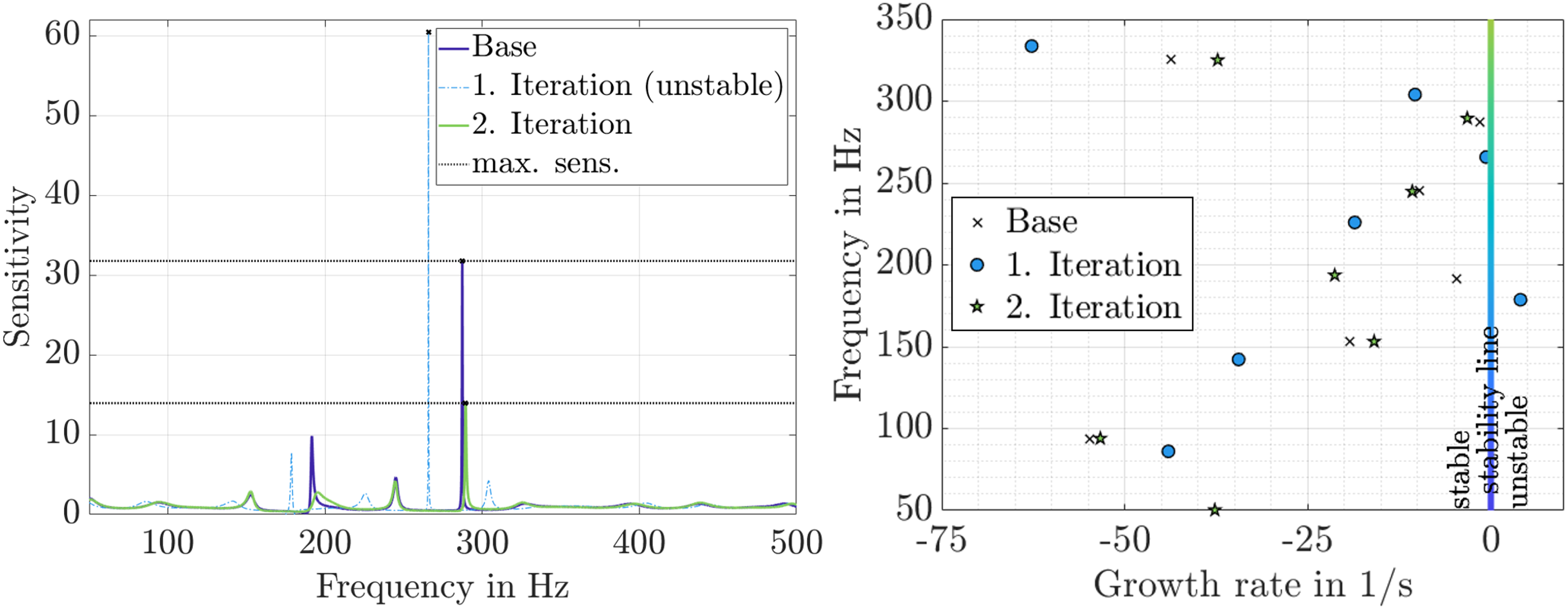
The results of the second case are shown in Figure 9. The left panel shows the sensitivity curves and the right panel the EVs for the first two iterations. A very high maximum sensitivity and a corresponding EV close to the stability limit is visible around 287 Hz in the baseline case. In the first iteration, the optimizer successfully modifies the FTF such that the sensitivity at this frequency is minimized. However, the modification of the FTF results in an unstable thermoacoustic system with an unstable mode at approximately 178 Hz. This is detected in the optimization routine as the real part of the corresponding Nyquist curve is $<1$ and the frequency of instability is added to the list. In the second iteration, the optimization routine restarts from the initial configuration but now considers 287 and 178 Hz within the DSM loop. As a result, the maximum sensitivity is successfully reduced without destabilizing the overall system. The optimization was performed for three more iterations, in which the maximum sensitivity could not be improved. Therefore, it can be assumed that the optimizer has converged to a (local) optimum. For clarity, the corresponding curves of subsequent iterations are not shown in Figure 9. The parameters associated with the best solution are $K=0.97$ and $x_i=-1.99$ . A possible reason why the optimizer can not identify more robust configurations in the following iterations is associated with the range of critical frequencies, which is around 180–350 Hz. As discussed in Figure 3, in this frequency range the contribution of velocity fluctuations, FTF _u , to the total FTF gain is low. Accordingly, the optimization parameter $K$ , which only affects FTF _u , is likely to have a small influence on the thermoacoustic EV spectrum. The value of the second optimization parameter (the location of fuel injection, $x_i$ ) on the other hand appears to be limited by the destabilization of modes at other frequencies. Thus, to have a greater impact on the stability margin, additional parameters would need to be varied. In summary, this second example shows that the algorithm can handle the occurrence of unstable EVs and still increase the stability margin. However, it also underlines that the possibilities of data-driven optimization are always limited by the influence of the chosen optimization parameters.

Figure 9.

Left: Sensitivities of the thermoacoustic system after each iteration of the optimization routine of Case 2. The dotted horizontal lines mark the maximal value of the starting configuration as well as the smallest maximum found during the optimization. Right: The corresponding eigenvalues at each iteration.

Furthermore, Case 2 shows a characteristic of the routine that is associated with the consideration of individual frequencies. In the second optimization run which starts from the baseline conditions, a distinct peak in the sensitivity function can be observed close to the original critical frequency. It is likely that this peak can be associated to the same eigenvalue which has only shifted slightly in frequency. However, as the optimization routine only reduces the sensitivity at the exact critical frequency and does not track distinct EVs, the shifted peak is not detected. Thus, small changes in the FTF that modify the frequency of EVs in the spectrum might be considered overly beneficial by the optimization routine. Adding more critical frequencies to the list of potentially critical frequencies during the iterations solves this problem as the optimization progresses. However, the algorithm first has to identify a sufficiently high number of critical frequencies in the first iterations before the system’s robustness is effectively increased.

Conclusions

In this study, a method for data-driven optimization of the flame response within a low-order network model is proposed and applied to a hybrid thermoacoustic model consisting of a Rijke tube acoustic and $G$ -equation based flame model. The method exploits the Nyquist criterion to compute a measure for thermoacoustic robustness which serves as a target value for the optimization. The objective of the algorithm is to decrease the maximum sensitivity of the thermoacoustic system by shaping the flame transfer function. Although data-driven optimization is typically associated with high costs, we minimized the amount of data required by evaluating only potentially critical frequencies, rather than evaluating the entire flame transfer function in every iteration.

Characteristics and challenges associated with the practical implementation of the data-driven optimization technique have been discussed using two example cases. Additional eigenvalue analysis showed that the methodology minimizes growth rates of EVs across the thermoacoustic spectrum by considering single critical frequencies. Without the need to determine EVs, a small number of simulations (or experiments) is sufficient to achieve maximum robustness of the thermoacoustic system. The method has thus the potential of being applied to experimental assessments of thermoacoustic stability and identifying optimal operating conditions within a relatively small number of experiments.