Flame dynamics in the lean burnout zone of an RQL combustion chamber - response to primary zone velocity fluctuations

Abstract

This study focuses on elucidating the flame dynamics of the lean burnout zone of an Rich-Quench-Lean (RQL) combustion chamber. With a new experimental approach of spatially separating the rich primary zone from the lean burnout zone, the latter can be investigated independently in terms of velocity fluctuations. Acoustically stiff mixing air ports in the lean burnout zone are ensured to prevent any acoustic interaction of the primary crossflow with the secondary mixing air jets. Therefore, defined boundary conditions at the mixing air inlets are used. Resulting no thermoacoustic interaction and additional flame dynamics are generated. In this specific case the lean burnout zone can be treated as a 2-port system allowing the application of existing evaluation methods e.g. acoustic determination of flame-transfer-functions (FTF) from the Rankine-Hugoniot (RH) equation or quantification of the heat release with chemiluminescence in combination with the Multi-Microphone-Method (MMM). Within this research, FTFs acoustically measured with the RH approach are presented and serve as a baseline for comparison with ones measured via a photomultiplier tube (PMT). It is found that the inverse diffusion flame in the burnout zone only reacts to fluctuations in the low frequency range and a clear low pass behavior is observed. The FTFs, calculated via the PMT match those from RH very well. Amplitude weighted phase images, recorded with a high-speed camera setup, visualize changes during excitation which complement and confirm the findings from the FTF.

Introduction

Due to increasing requirements for environmental protection, the regulations for carbon dioxide emissions from aircraft engines become stricter year to year. Within the German federal research program ‘Luftfahrtforschungsprogramm des Bundes’, the development of innovative technologies for aero-engines to reduce carbon dioxide and NOx emissions is strongly supported. Various low-emission combustion systems have already been developed and are the focus of many research studies. The RQL (rich-quench-lean) combustor is an effective method to control carbon dioxide and NOx emissions. Within an RQL combustor, the combustion process starts in the primary fuel rich zone close to the injector, followed by an air quenching, fuel lean secondary zone to complete the combustion process. Regions close to stoichiometric conditions where NOx production is expected to be highest, are minimized.

Holdeman, ¹ Rosfjord et al. ² tested an RQL combustion chamber with a cylindrical flame tube and geometrical variations in quench jet-in-crossflow (JIC) configuration to evaluate the ability of RQL combustors to achieve low emissions. The results showed that emissions were highly sensitive to the performance of the quench and mixing zone and less sensitive to the performance of the injector. Efficient mixing and dilution of the fuel rich mixture is key for a successful low emission RQL combustor. Multiple experimental and numerical studies for the secondary zone followed, focusing on the flowfield, the mixing and reaction processes and the determination of its main influencing factors. Holdeman ¹ identified the momentum-flux ratio (J) as well as orifice geometry and spacing as one of the crucial parameters influencing the mixing, combustion and emission processes.

Like all high power density combustors RQL combustion is prone to thermoacoustic instabilities, caused by the coupling of unsteady heat release and acoustic oscillations. One of the first experimental studies on the dynamics of RQL combustors was published by Eckstein et al. ³ . The main objective of this research was the low-frequency phenomenon called ”rumble”, which is observed in aero engines at idle and sub-idle conditions. The research was focused on the response of a spray flame in an RQL combustor only to primary air forcing and on the entropy-wave interaction with the combustor exit nozzle. Eckstein ⁴ related most of the findings to the atomization and spray evaporation process. With his setup the contribution of the mixing and dilution zone to the dynamic response of the total RQL combustor could not be shown. Without downstream acoustic forcing (available in later studies e.g.^5–7) the quantitative determination of the thermoacoustic response, e.g. as flame-transfer-matrix (FTM) or flame-transfer-function (FTF) was not possible. However, it is conceivable that the thermoacoustic behavior of the lean combustion zone plays a decisive role for the overall combustion dynamics of RQL combustors. Cai et al. ⁸ investigated the dynamics of an RQL combustor segment operating at ambient pressure with natural gas. They identified instabilities in the lean and the RQL operation mode. Using chemiluminescence heat release images and dynamic pressure measurements inside the chamber, a correlation of the acoustic emissions in the RQL operation mode and the interaction of the fuel-rich mixture from the rich zone with the secondary air jets was shown. Cai et al. ⁸ could not quantify these dynamics in an FTF.

The novel test rig presented in the authors previous paper ⁹ was designed to measure and characterize the flame dynamics of the lean secondary zone in an RQL combustion chamber. Separating the rich primary zone from the lean mixing zone allows an independent investigation of the lean secondary zone and its contribution to the whole acoustic system.

This paper is structured as follows. First, the RQL topology is discussed in terms of acoustic network elements. Ensuring acoustically stiff mixing ports reduces the complexity of the test rig and known methodological techniques can be applied. Next, the experimental setup approaching such a 2-port system is described and the operation range is discussed. The measurement methods and evaluation procedure are given, including the computation of the flame images and the two operation modes of the test rig for the determination of the flame-transfer-matrix (FTM). Finally, multiple FTFs are presented and the dynamic behavior is discussed.

Thermoacoustic theory of RQL combustors

The network technique^10,11 is a common tool for the identification and description of the thermoacoustic properties of combustion systems. In the network, the thermoacoustic element describes the functional relations between the acoustic variables, e.g. acoustic pressure and acoustic velocity, at its ports based on the conservation equations and element specific transfer functions representing e.g. acoustic losses or flame transfer functions. In the well established method for 2-port elements (e.g.^5–7,12) the dynamics of flames are represented using linearized Rankine-Hugoniot (RH) relations into which the specific flame dynamics enter as the flame transfer function (FTF) forming a $2\mathrm{x}2$ complex flame transfer matrix (FTM). Together with the 2-port burner transfer matrix (BTM) this allows representation of the dynamics of the burner and flame as an effective 2-port system, the burner flame transfer matrix.

$$\mathrm{BFTM}=\mathrm{FTM}\cdot \mathrm{BTM}$$

(1)

For the identification of the BTM (without flame) and the BFTM (with flame) acoustic forcing of the upstream and downstream port is used together with the Multi-Microphone-Method (MMM) to determine the acoustic variables at these stations. Using the BFTM and BTM determined from the MMM technique, equation 1 can be solved for the FTM

$$\mathrm{FTM}=\mathrm{BFTM}\cdot {\mathrm{BTM}}^{-1}$$

(2)

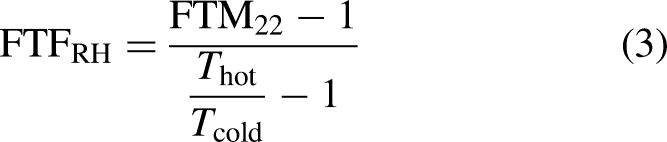
The linearized RH relations for pressure and velocity across the flame are derived from the conservation equations of mass, momentum and energy. ¹³ The FTF is commonly obtained from the (2,2)-element of the FTM as

$${\mathrm{FTF}}_{\mathrm{RH}}=\frac{{\mathrm{FTM}}_{22}-1}{\frac{T_{\mathrm{hot}}}{T_{\mathrm{cold}}}-1}$$

(3)

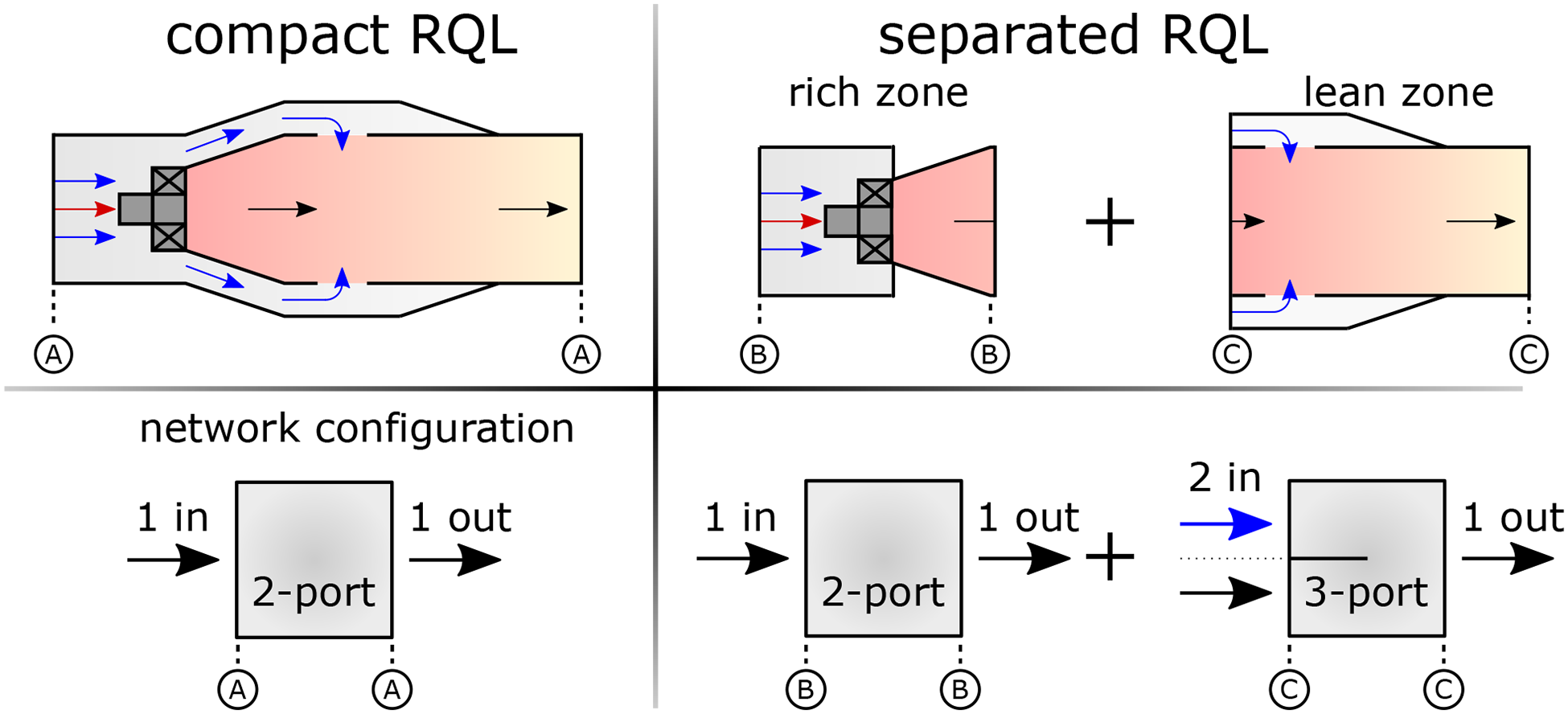
In this equation, $T_{\mathrm{cold}}$ and $T_{\mathrm{hot}}$ are temperatures before and after the flame which characterize the expansion of the flow by the combustion heat release. How they are determined for the secondary zone considered in this paper is discussed below in the measurement methods section. By selecting the physical location of the ports as shown in Figure 1 on the left, the compact RQL combustor can formally be addressed as a 2-port system ( $◯\mathrm{A}-◯\mathrm{A}$ ). However, in this case the flame dynamics of the primary and secondary zones are inseparable. The aim of the current research is the identification and description of the individual flame dynamics of the primary and the secondary zones of an RQL combustor by separating them to allow the identification of either zone as seen in Figure 1 on the right. This arrangement is referred to as the separated RQL. The split into the separated RQL now produces a 2-port system for the primary zone ( $◯\mathrm{B}-◯\mathrm{B}$ ), which can be treated by the established 2-port technique. But the secondary zone now forms a 3-port system connecting the primary zone, the secondary mixing air holes and the burnout zone ( $◯\mathrm{C}-◯\mathrm{C}$ ).

Figure 1.

Comparison of combustion chamber topology between compact and separated arrangement in terms of a network element approach.

The basic technique for the network treatment of 3-ports was proposed by Karlsson and Åbom ¹⁴ and Holmberg et al. ¹⁵ . They describe the 3-port by a $3\times 3$ matrix which can be determined by three acoustically independent measurements, which provide the equations for the 9 unknown complex matrix elements. In the current research this form is extended by introducing a RH-type flame-transfer-function and separating its response into two parts. One responding to the fluctuations from the primary zone port and the other to those of the secondary air mixing port. The detailed development of this technique will be published in a future paper. At this point, asymptotic cases can be identified, in which the 3-port system degenerates into a 2-port system and can readily be analyzed using the established MMM 2-port technique. Theses cases will serve to validate the generalized 3-port technique outlined above. One of these asymptotic cases is formed by acoustically stiff secondary mixing air holes and this is investigated experimentally in this paper.

Experimental setup

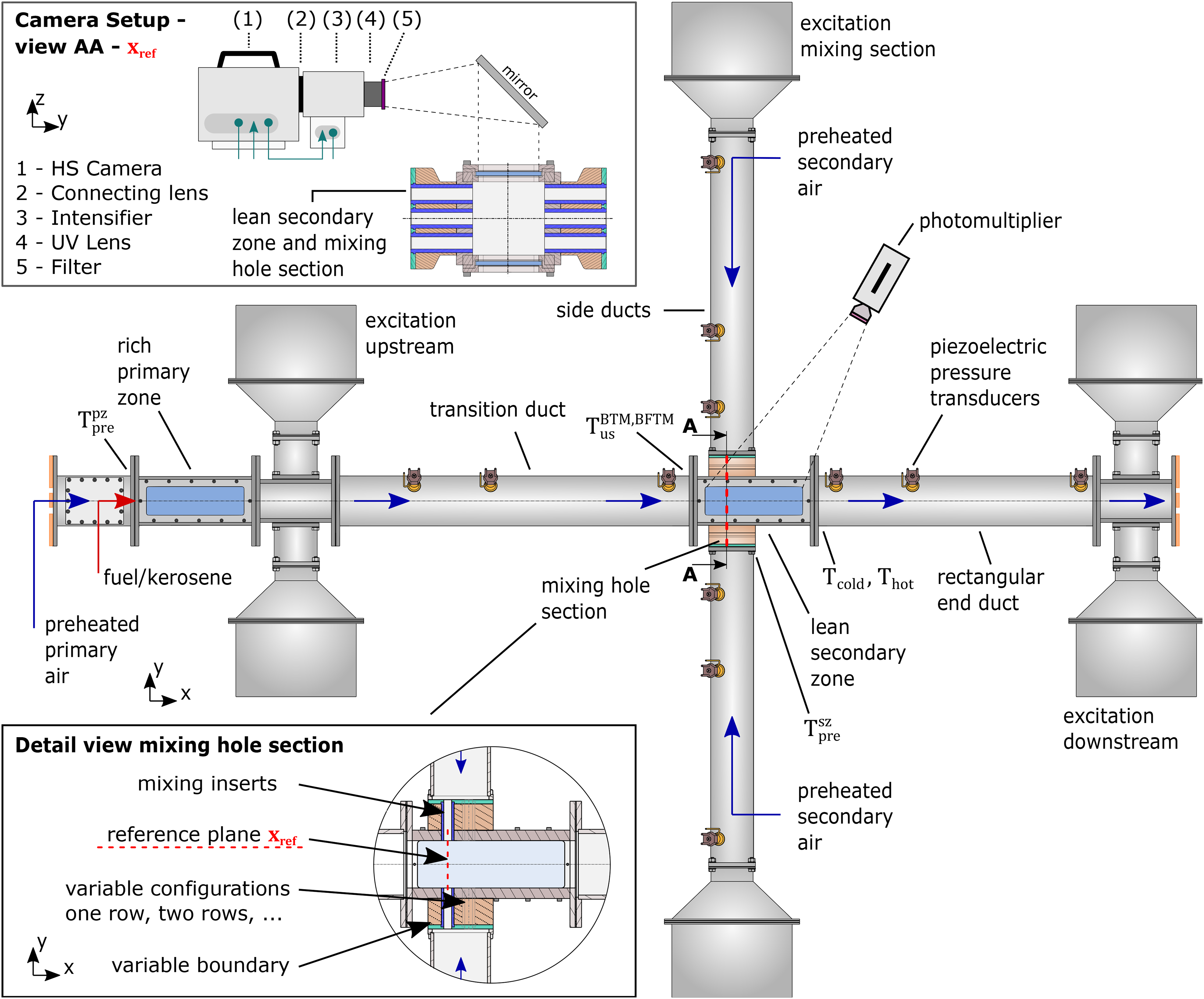
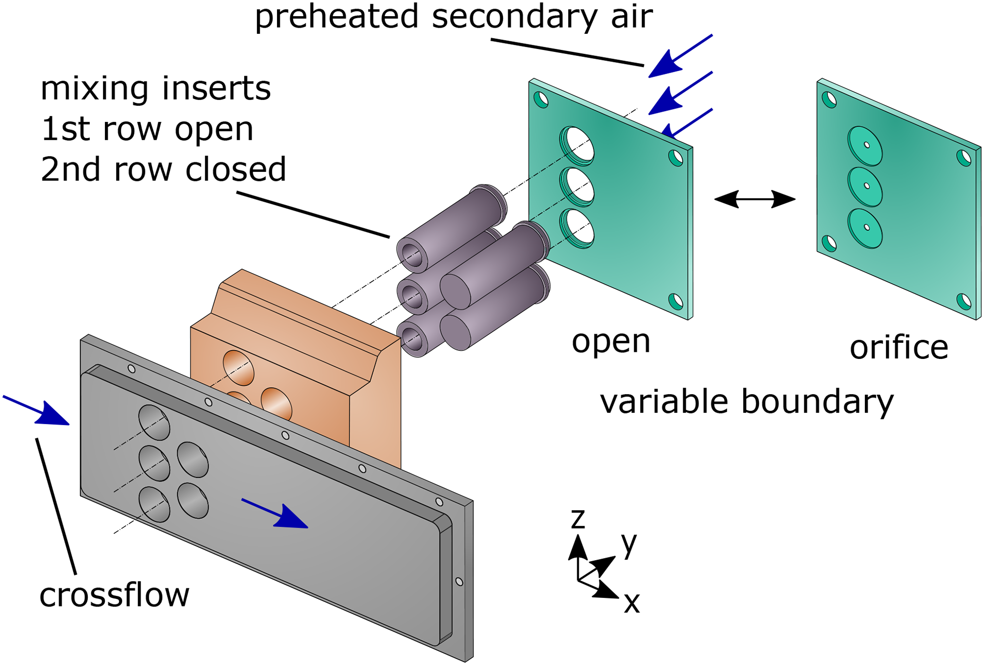
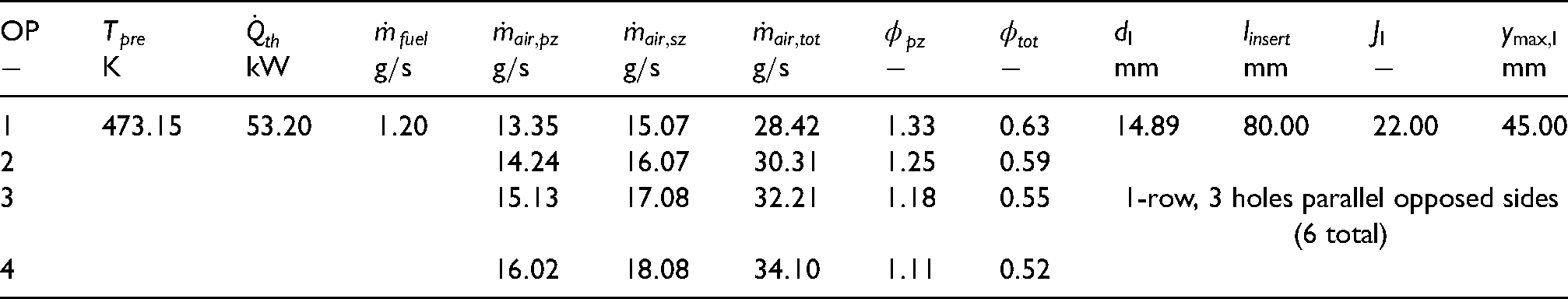
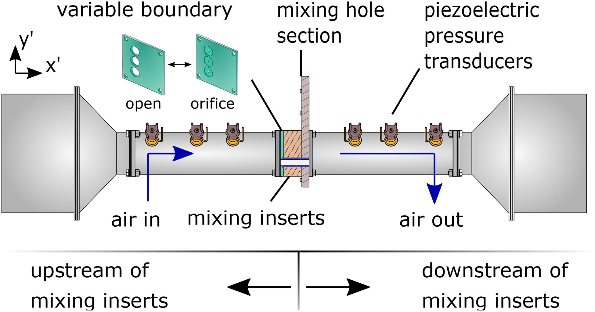
The Experiments were performed on the RQL test rig shown in Figure 2. The test rig operates at atmospheric pressure in a thermal power range of 45–80 kW. The total air mass flow rate is divided into separately measured and preheated primary and secondary air flows. The primary air flow enters the test rig on the left with a constant inlet temperature of $T_{pre}^{\mathit{\text{,pz}}}=473\mathrm{K}$ , measured with a thermocouple Typ-K as indicated in Figure 2. The primary combustion chamber is equipped with a generic fuel injector, which can be operated with kerosene as a liquid fuel as well as with gaseous fuels. The primary combustion chamber has a $90\mathrm{x}90{\mathrm{mm}}^2$ square cross-section and a total length of $l_{cc}=0.28\mathrm{m}$ . It is followed by the upstream excitation element with two loudspeakers (Type: Eminence Kappa $12\text{in}$ ). The transition duct is used to reconstruct the 1D acoustic field and has a length of $l_{td}=0.96\mathrm{m}$ and a diameter $d_{td}=0.117\mathrm{m}$ and connects excitation element to the lean secondary combustion chamber. Three dynamic pressure transducers are mounted at non-equidistant spacing to ensure high quality wavefield reconstruction with the MMM in the transition duct.^16–19 The lean secondary combustion chamber has a geometry similar to the primary zone with $90\mathrm{x}90{\mathrm{mm}}^2$ , $l_{cc}=0.28\mathrm{m}$ and is optically accessible. The preheated secondary air $T_{pre}^{\mathit{\text{sz}}}=473\mathrm{K}$ is also measured with a thermocouple Typ-K and enters the test rig through the two side ducts mounted to the secondary zone. The side ducts with $l_{side}=0.85\mathrm{m}$ and $d_{side}=0.112\mathrm{m}$ are used for the MMM technique and are connected to the lean combustion chamber via the mixing hole section shown in Figure 3. Using inserts allows variation of the hole geometry, the number of rows and the pattern within the mixing hole section. The current setup is shown in Figure 3 and the design parameters are listed below in Table 1. More information about the design of the mixing holes can be found in March et al. ⁹ . For the measurements presented in this paper, a single row setup consisting of three opposed mixing holes on each side was chosen. Compared to the wavelength of the investigated low frequency range the inserts are expected to be compact. Acoustic excitation of the mixing holes and application of the MMM is possible on both sides of the chamber with loudspeakers at the end of the side ducts. The secondary zone is followed by a rectangular end duct with the same side length as the combustion chamber and a total length of $l_{ed}=0.92\mathrm{m}$ . As for the transition duct and the side ducts, non-equidistant spaced pressure transducers are mounted and a downstream excitation element is used to perform acoustic forcing. A perforated plate at the end of the test rig provides a low acoustic reflection coefficient. For acoustic measurements, the test rig is equipped with 12 water-cooled Synotech PCB 106B piezoelectric dynamic pressure transducer located in the transition, side and end ducts. In addition, a photomultiplier tube (PMT) is employed for chemiluminescence measurements. The PMT is mounted above the lean secondary zone and views the frame through the upper quartz glass window. A narrow bandpass filter with a wavelength of $308\mathrm{nm}$ full width at half maximum of $10\mathrm{nm}$ is used to detect emissions in the ${\text{OH}}^{*}$ band. Dynamic pressure and the PMT data are recorded at a sample rate of $f_s=65536$ samples per second. A total of $n_s=524288$ samples are recorded for each excitation frequency in the range of $60\mathrm{Hz}\text{-}400\mathrm{Hz}$ with a frequency step of $10\mathrm{Hz}$ . To locally resolve the detailed flame shape, an intensified high speed (HS) camera (Photron FastCam SAX) equipped with the same type of interference filter as applied for the PMT observes the flame via a mirror and the quartz glass window. The HS camera setup is depicted in the upper left corner of Figure 2 and the procedure will be explained in detail in the measurement methods section.

Figure 2.

Atmospheric RQL test rig - Top view setup for secondary zone; upper left: setup of the high speed camera for phase-resolved chemiluminescence intensity measurements and view of cut-plane AA; lower left: detailed view of mixing hole section and position of reference plane $x_{\mathrm{ref}}$ .

Figure 3.

Mixing hole section setup; view of mixing inserts and variable boundary.

Table 1.

Operating range and mixing hole section.

OP	$T_{pre}$	${\dot{Q}}_{th}$	${\dot{m}}_{fuel}$	${\dot{m}}_{air,pz}$	${\dot{m}}_{air,sz}$	${\dot{m}}_{air,tot}$	${\varphi }_{pz}$	${\varphi }_{tot}$	$d_{\mathrm{I}}$	$l_{insert}$	$J_{\mathrm{I}}$	$y_{\max ,\mathrm{I}}$
$-$	$\mathrm{K}$	$\mathrm{kW}$	$\mathrm{g}/\mathrm{s}$	$\mathrm{g}/\mathrm{s}$	$\mathrm{g}/\mathrm{s}$	$\mathrm{g}/\mathrm{s}$	$-$	$-$	$\mathrm{mm}$	$\mathrm{mm}$	$-$	$\mathrm{mm}$
$1$	$473.15$	$53.20$	$1.20$	$13.35$	$15.07$	$28.42$	$1.33$	$0.63$	$14.89$	$80.00$	$22.00$	$45.00$
$2$				$14.24$	$16.07$	$30.31$	$1.25$	$0.59$
$3$				$15.13$	$17.08$	$32.21$	$1.18$	$0.55$	1-row, 3 holes parallel opposed sides (6 total)
$4$				$16.02$	$18.08$	$34.10$	$1.11$	$0.52$

Acoustically stiff mixing air jets

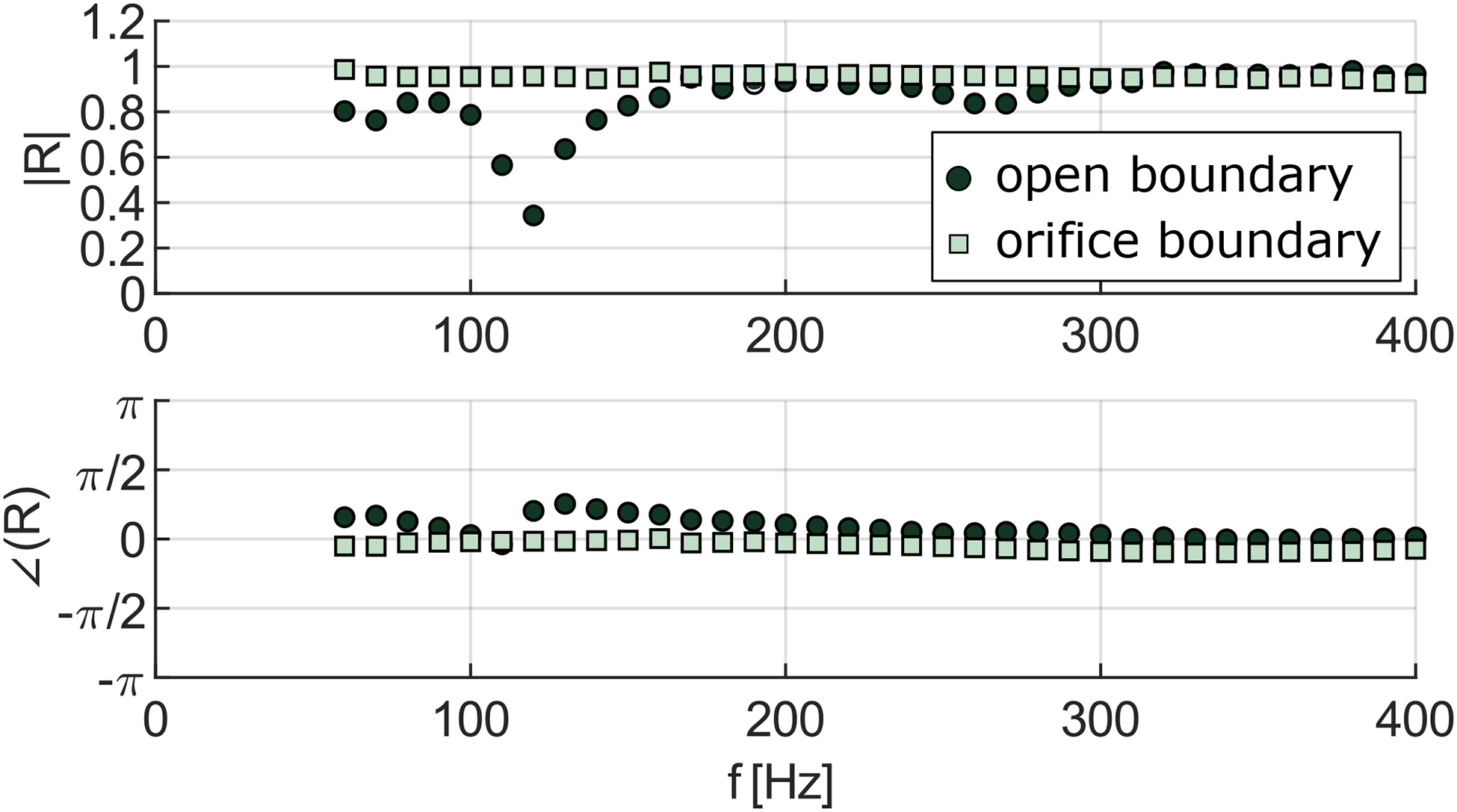
In order to reduce the acoustic 3-port system to an acoustic 2-port system, the acoustic fluctuations of the mixing air jets must be suppressed. This was achieved using choked orifices in place of open insert holders at the entrance to the inserts as illustrated in Figure 3. This was tested in the simplified setup shown in Figure 4. Figure 5 shows the reflection coefficient of the downstream side of the inserts measured for both configurations. The open insert configuration, marked with circle symbols, results in the reflection coefficient $R$ with local minimum at $f=120\mathrm{Hz}$ with $|R|=0.34$ . Towards higher frequencies the reflection coefficient rises and settles around $|R|=0.91$ . Changing the boundary to the choked orifices results in a reflection coefficient of $|R|>0.91$ for the entire frequency range and marked with the square symbols. Based on this, the velocity fluctuations in the mixing holes of the test rig can be assumed to be very close to zero $u_{\mathrm{side}}^{\mathrm{\prime }}=0$ . This allows the reduction of the test rigs acoustic topology from a 3-port, to a 2-port system.

Figure 4.

Simplified test section for characterization of mixing hole section with variable boundaries.

Figure 5.

Reflection coefficient determined at simplified test section in mixing holes.

Measurement methods

Operating modes and conditions

Extracting the transfer matrices and the ${\mathrm{FTF}}_{\mathrm{RH}}$ from measurement data requires two independent data sets for each operation mode. In the case with flame in secondary zone (BFTM), the hot and partially burned mixture ( ${\varphi }_{\text{,pz}}>1$ ) from the primary zone will further react in form of an inverse diffusion flame as soon as the secondary air flow is added. For each operating point, the inlet temperature $T_{\mathrm{us}}^{\mathrm{BFTM}}$ of the secondary zone is measured and serves as the target for the BTM measurements. Typically BTM measurements are performed with preheated air flowing through the burner. In the presented case the inlet temperatures at the secondary zone from upstream are too high for the use of air preheaters. Therefore the BTM is measured with the same secondary air settings but operating the primary zone at lean ( ${\varphi }_{\text{,pz}}<1$ ) conditions at the same total flow rate. The flow temperature is then controlled by changing the fuel mass flow rate until the inlet temperature of the secondary zone in the BTM case equals the target temperature from the reactive BFTM case $T_{\mathrm{us}}^{\mathrm{BTM}}=T_{\mathrm{us}}^{\mathrm{BFTM}}$ .

RH flame temperatures

The flame front is considered as a discontinuity of negligible thickness, which adds heat to the flow between the constant temperatures before ${\mathrm{T}}_{\mathrm{cold}}$ and downstream ${\mathrm{T}}_{\mathrm{hot}}$ of the flame. ²⁰ The temperatures in the denominator of equation 3 are measured in the two cases with and without flame using thermocouples of Typ-N. In this study, fuel (crossflow) and oxidizer (mixing air) enter the secondary zone separately. Mixing then takes place by convection and diffusion. Combustion occurs in a thin layer in the vicinity of the mixture surface. Here, the local mixture fraction gradient is sufficiently high thus this surface is defined by a most reactive mixture fraction $Z_{\mathrm{mr}}$ and a corresponding mixture temperature $T_{\mathrm{mr},\mathrm{mix}}$ . The latter is the starting point of the combustion and is interpreted as the temperature $T_{\mathrm{cold}}$ in equation 3. $T_{\mathrm{cold}}$ is measured in the BTM case where pure mixing takes place. $T_{\mathrm{hot}}$ in equation 3 is measured in the BFTM case with flame.

Chemiluminescence

Since the hot gases from the primary zone are highly reactive (hot and high hydrogen content), it can be expected that the secondary flame will react in a flamelet regime with a narrow stoichiometry band around the most reactive mixture fraction. In this case the chemiluminescence of the flame would, similarly to premixed combustion, be a function of the flamelet density and could serve as a measure of the heat release. In this investigation, the ${\text{OH}}^{*}$ -radical is used as a representative to measure the fluctuating heat release. A second FTF formulation can than be obtained in combination with the MMM where velocity fluctuations are measured at the reference position. From this, a hybrid formulation of the FTF can be evaluated.

$${\mathrm{FTF}}_{\mathrm{PMT}}=\frac{I_{\mathrm{O}{\mathrm{H}}^{*}}^{\mathrm{\prime }}/{\overline{I}}_{\mathrm{O}{\mathrm{H}}^{*}}}{u_{\mathrm{ref},\mathrm{us}}^{\mathrm{\prime }}/{\overline{u}}_{\mathrm{ref},\mathrm{us}}}$$

(4)

As described in the experimental setup, the ${\text{OH}}^{*}$ PMT is mounted above the test rig and captures the flame chemiluminescence during the forcing cycle simultaneously with the pressure transducers. ${\text{OH}}^{*}$ chemiluminescence has become widely used for heat release in premixed flames and has been extended to non-premixed combustors by. ²¹ Most approaches relying on chemiluminescence are prone to regions of high strain and strong equivalence ratio fluctuations. The latter provides an additional influence to the heat release and thus the FTF often cannot be calculated correctly from the ${\text{OH}}^{*}$ -radical chemiluminescence. ²² On the other hand, ²³ proved that the use of chemiluminescence is able to capture the heat release of turbulent flames with a classic burner-flame setup. Despite of this encouraging results, it is not clear to what extent ${\text{OH}}^{*}$ chemiluminescence is representative of the heat release rate in the specific case of the lean inverse diffusion flame of the secondary zone presented here. For this reason, the FTF found with the ${\text{OH}}^{*}$ chemiluminescence method is compared with the one measured with the pure acoustic approach (RH) in the results chapter, which is considered as baseline.

Computation of flame images

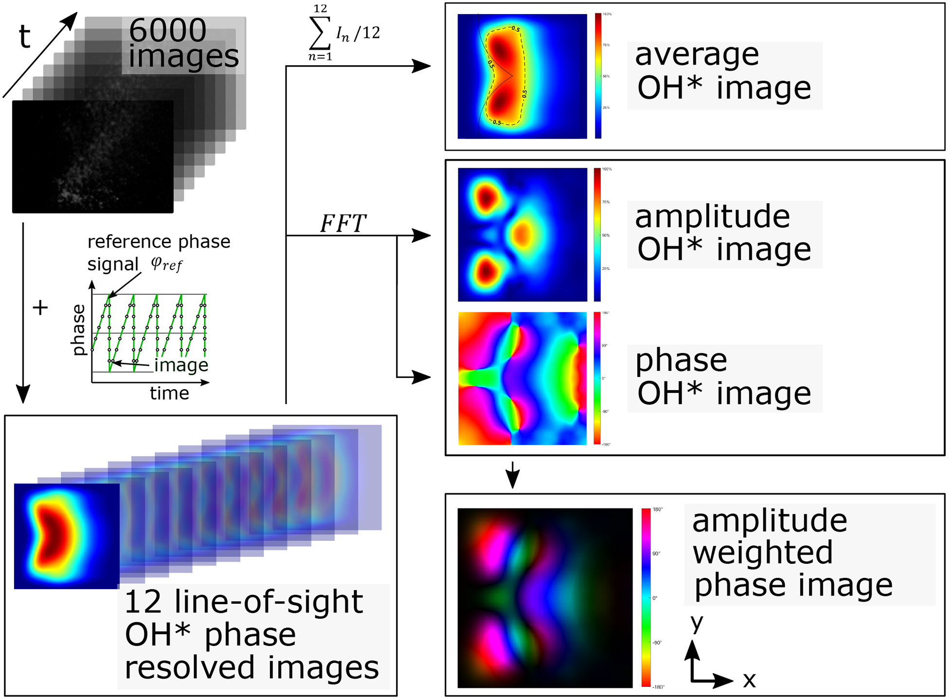
To locally resolve the detailed flame shape, an intensified high speed (HS) camera (Photron FastCam SAX) equipped with the same type of interference filter as applied for the PMT observed the flame via a mirror and the quartz glass window. The setup is shown in Figure 2 in the upper left. Given the restrictions described above, the HS chemiluminescence images are only used as a qualitative indication of the spatial heat release distribution. To ensure that a sufficient depth of field is in sharp focus, a aperture setting of $\mathit{f}=2.8$ is applied for the $45\mathrm{mm}$ UV lens with sufficient intensifier gain to compensate for the reduction of light passing through the lens and the low flame intensity. The logical trigger signals for the camera record sequence and intensifier gating are sampled synchronously to the dynamic pressure measurements. This permits the assignment of a precise time stamp for each image relative to the pressure signal and allows phase-resolved investigation of the flame dynamics. To achieve sufficient temporal resolution of the flame dynamics, images are sampled at a rate of $6000$ frames/s. This results in $500$ images per phase angle.^4,24,25 The post processing of the phase-resolved flame images is illustrated in Figure 6. Cropping and ensemble averaging the timeseries produces 12 phase-resolved images. Subsequently, an FFT for each pixel is performed, calculating the amplitude and phase value. From the resulting amplitude image, the areas with high intensity fluctuation can be identified, with brightness being proportional to amplitude. The phase image gives the temporal relation of the intensity fluctuations to each other in relation to the reference signal. A color code from red ( $-\pi$ ) via yellow, blue ( $0$ ) and green back to red ( $+\pi$ ) is used. Weighted phase images show both results in one plot, where the phase is encoded by the color-coding and the amplitude by the brightness.

Figure 6.

Schematic illustration of the image processing used to create the mean value image, the 12 phase-resolved images and the amplitude weighted phase image.

Results

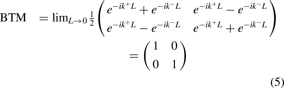
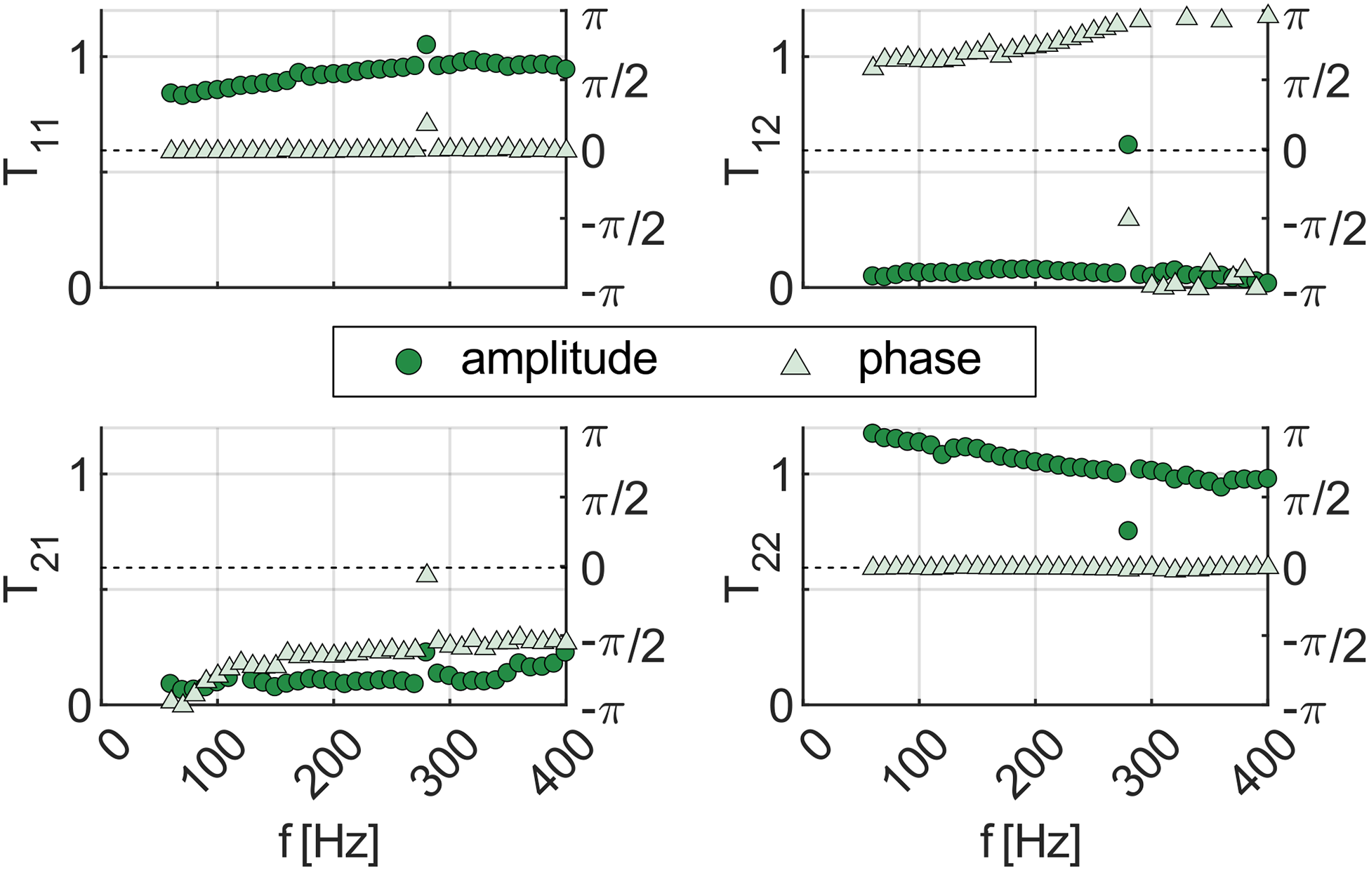
In the following the location of the two ports of the transfer matrices, also referred to as reference planes, are defined at the same position $x_{\mathrm{ref}}$ . $x_{\mathrm{ref}}$ is the axial location of the cross section through the secondary air inserts and is marked in Figure 2. An illustrative example of a measured BTM is shown in Figure 7, with normalized pressure $p^{\prime }/\rho c$ and velocity $u^{\prime }$ for OP2. The secondary zone can be approximated as a straight duct with rectangular cross section and infinitesimal small length. Therefore, one would expect an analytical transfer matrix in form of equation 5.

$$\begin{array}{r}\begin{array}{cc}\mathrm{BTM}& =\underset{L\to 0}{lim}\frac{1}{2}\left(\begin{array}{cc}{e}^{-i{k}^{+}L}+e^{-i{k}^{-}L}& e^{-i{k}^{+}L}-e^{-i{k}^{-}L}\\ e^{-i{k}^{+}L}-e^{-i{k}^{-}L}& e^{-i{k}^{+}L}+e^{-i{k}^{-}L}\end{array}\right)\\ & =\left(\begin{array}{cc}1& 0\\ 0& 1\end{array}\right)\end{array}\end{array}$$

(5)

The absolute value of the element $T_{11}$ , which relates the pressure upstream and downstream of the reference position, is close to unity. The phase matches the expected value of zero since the reference position $x_{\mathrm{ref}}$ is geometrically compact. The element $T_{12}$ shows the influence of the upstream velocity on the downstream pressure and thus can be interpreted as a pressure loss term. The $T_{21}$ element relates the upstream pressure to the downstream velocity and is expected to be small. The phase deviations have a negligible impact on the response due to the small magnitude of the element. Element $T_{22}$ connects the acoustic velocity upstream and downstream and has a value of approximately one. This property results from the continuity equation for compact elements. Changes in the operating conditions do not affect any elements and as a result the other burner transfer matrices are similar and not shown here.

Figure 7.

Burner transfer matrix of operation point OP2, measured acoustically.

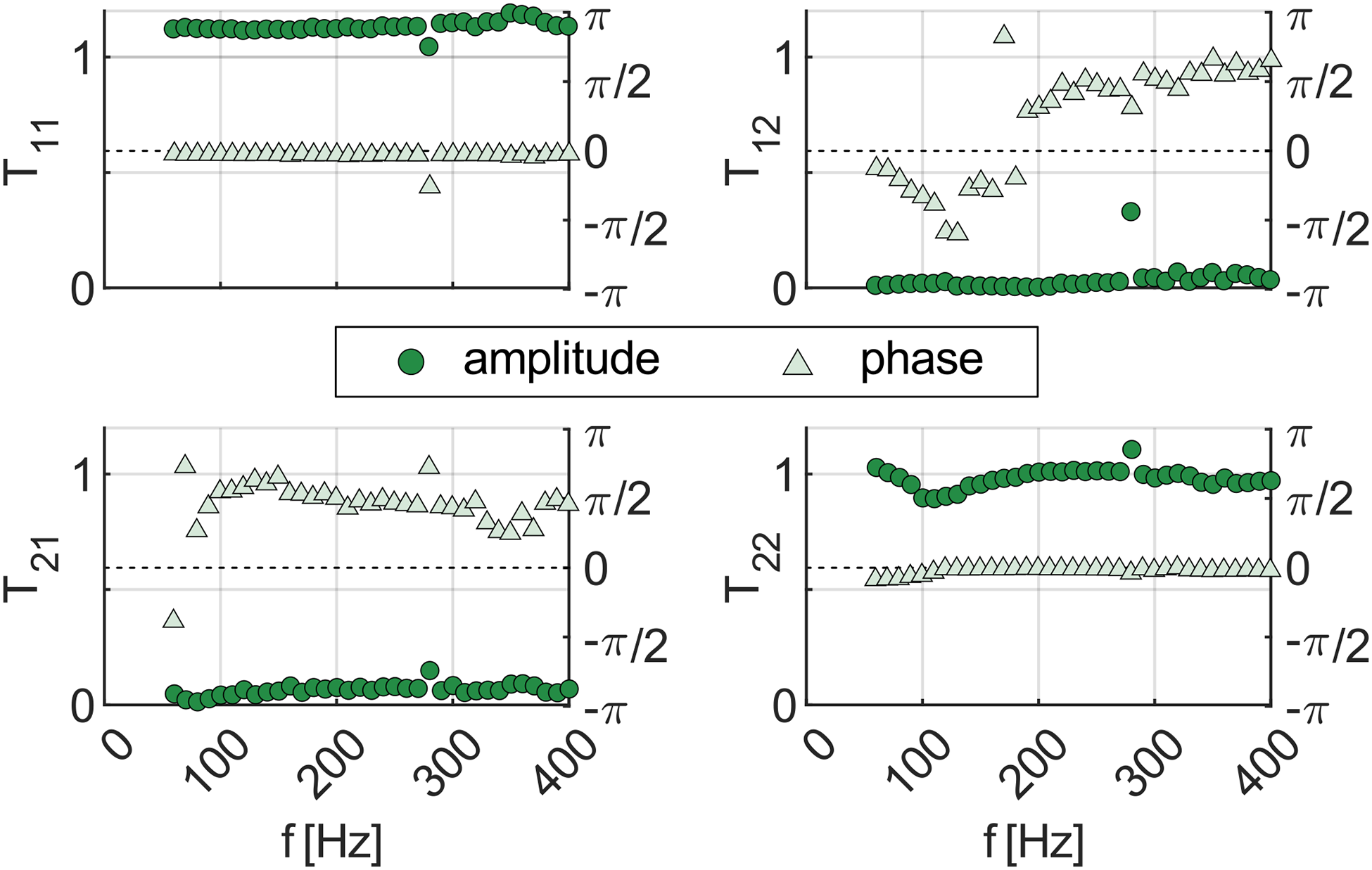
The BTM results are in good agreement with expectations. Next, the burner-flame transfer matrix is measured and the flame transfer matrix (FTM) is calculated using equation 2. Figure 8 shows the resulting FTM for one operation point OP2. The element $T_{11}$ has an almost constant absolute value which is close to the ratio of the characteristic impedances upstream $(\rho c{)}_{\mathrm{us}}$ and downstream $(\rho c{)}_{\mathrm{ds}}$ of the flame and a zero phase lag. The elements $T_{12}$ and $T_{21}$ are expected to have small amplitudes compared to the other elements, and therefore, the phase of these elements is not important. The element $T_{22}$ correlates to the fluid expansion due to the unsteady heat release rate and is highly dependent on the flame. Similar FTM results were found for the other conditions.

Figure 8.

Flame transfer matrix for one operation point OP2, calculated from BTM and BFTM measurements.

With the application of the Rankine-Hugoniot relations (equation 3), the ${\mathrm{FTF}}_{\mathrm{RH}}$ were calculated from the pure acoustic measurements. The hybrid ${\mathrm{FTF}}_{\mathrm{PMT}}$ gained from optical ${\text{OH}}^{*}$ PMT measurements will be compared against the ${\mathrm{FTF}}_{\mathrm{RH}}$ .

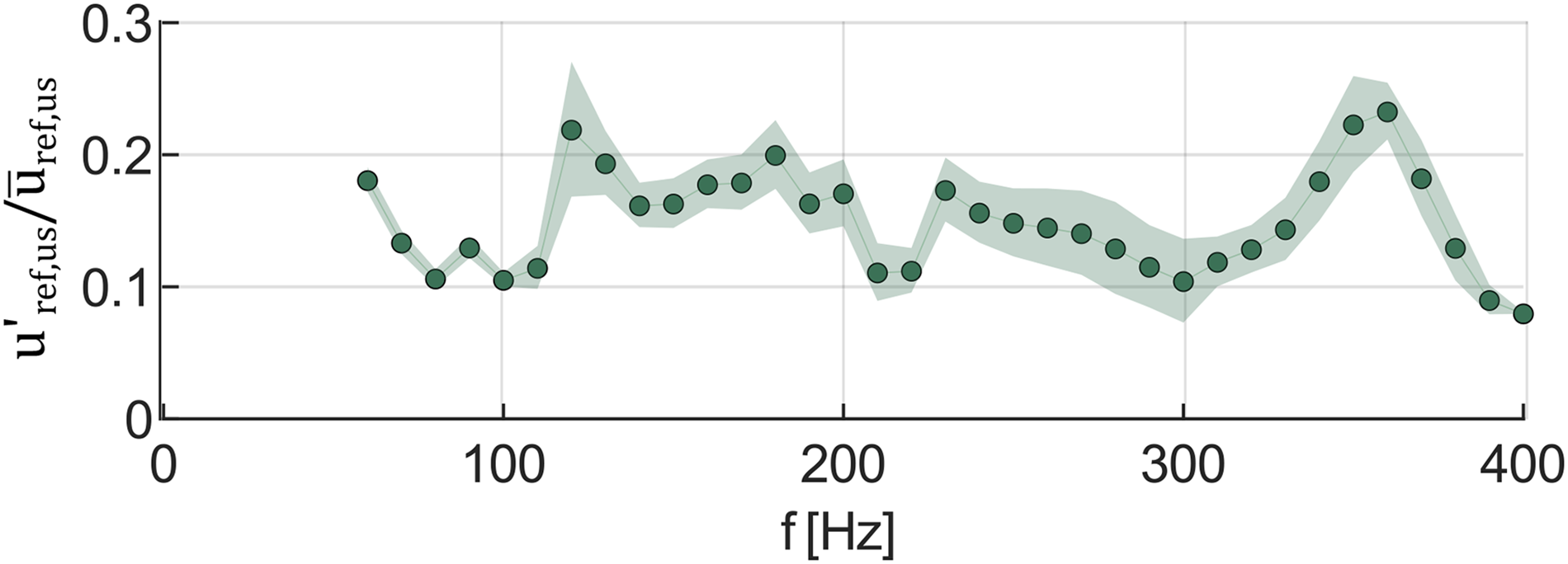
For the hybrid ${\mathrm{FTF}}_{\mathrm{PMT}}$ the flame was acoustically excited from upstream. The velocity fluctuations $u_{\mathrm{ref},\mathrm{us}}^{\mathrm{\prime }}$ were calculated using the multi-microphone method in the transition duct. To ensure that the flame response is in the linear regime, the forcing amplitude for all measurements was set between $10-20\text{\%}$ in terms of the normalized velocity fluctuations and is shown in Figure 9. The shaded surface in light green shows the standard deviation for all operation points.

Figure 9.

Velocity fluctuations (green markers) at the reference position upstream with the standard deviation (shaded light green surface) for the operating range.

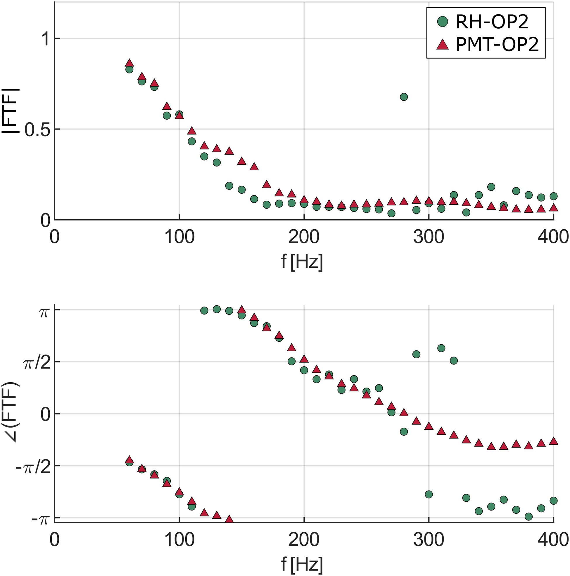
The results for the flame transfer function are plotted in Figure 10. It can be observed that both FTFs have absolute values decreasing from $|\mathrm{FTF}|=0.8$ at $f=60\mathrm{Hz}$ to very low amplitude values of $|\mathrm{FTF}|=0.14$ for frequencies higher $f=200\mathrm{Hz}$ . For the low frequency limit $f\to 0$ , the amplitude can be extrapolated towards $|\mathrm{FTF}|\approx 1$ and the phase becomes $\mathrm{\angle }\mathrm{FTF}\approx 0$ , like in technical premixed flames with choked fuel feed as found by.^5,12 The amplitude is indicating a more quasi-stationary thermal power modulation for low frequencies. The linear falling phase slope speaks for a constant convective time delay between the velocity fluctuations in the reference plane and the heat release in the inverse diffusion flame.

Figure 10.

Flame transfer function of OP2, pure acoustic ${\mathrm{FTF}}_{\mathrm{RH}}$ (green circles) compared with hybrid ${\mathrm{FTF}}_{\mathrm{PMT}}$ (red triangles); upper: amplitude of the FTFs; lower: phase angle of the FTFs.

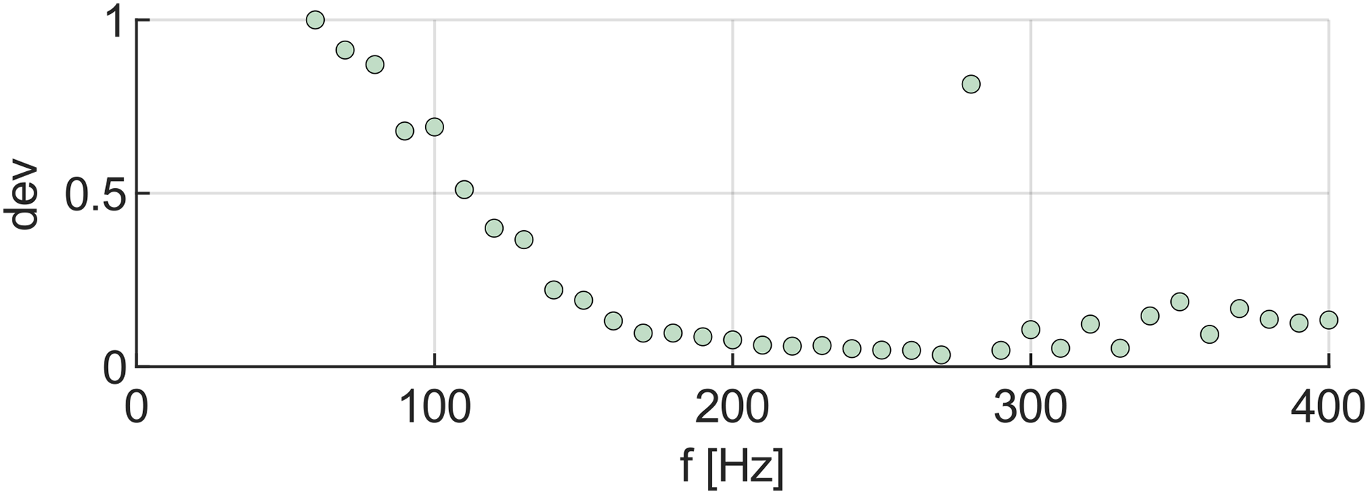
The scattering of the phase of RH-OP2 for higher frequencies results from the small ratio between the underlying BFTM and BTM data. Figure 11 shows the deviation of the ${\mathrm{T}}_{22}$ -element of the BFTM and BTM for OP2. Low values represent only small changes between the two measurements with and without flame. At higher frequencies, the MMM reaches its limits which results in the high scattering. Nevertheless, the PMT is not prone to those small changes and the PMT-OP2 shows a continuous falling phase slope till $f=400\mathrm{Hz}$ . Comparing the absolute values from RH-OP2 and PMT-OP2, one must pay attention to the temperatures used in the Rankine-Hugoniot equation 3. For the selected operation point, the reactive exhaust gases enter the secondary zone with $T_{\mathrm{in}}^{\mathit{\text{sz}}}=1134\mathrm{K}$ . After mixing with preheated secondary air with $T_{pre}^{\mathit{\text{sz}}}=473\mathrm{K}$ , the starting temperature of the mixture for combustion in the shear layers is the ideal mixing temperature $T_{\mathrm{id}.,\mathrm{mix}}=T_{\mathrm{cold}}=813\mathrm{K}$ . After the rich combustion in the primary zone, only $10-25\text{\%}$ of fuel remains for additional heat release in the lean secondary zone. This leads to low flame temperatures up to $T_{\mathrm{hot}}=1042\mathrm{K}$ . The small temperature increase from $T_{\mathrm{cold}}\to T_{\mathrm{hot}}$ makes the ${\mathrm{FTF}}_{\mathrm{RH}}$ sensitive to measurement errors. As the deviation between RH-OP2 and PMT-OP2 is small the authors are confident that the temperature measurements for the ${\mathrm{FTF}}_{\mathrm{RH}}$ calculation have sufficient accuracy. The same applies for the other operation points.

Figure 11.

Deviation $\mathrm{dev}=|\frac{{\mathrm{BFTM}}_{22}-{\mathrm{BTM}}_{22}}{max({\mathrm{BTM}}_{22})}|$ of the BFTM and BTM $T_{22}$ element for OP2.

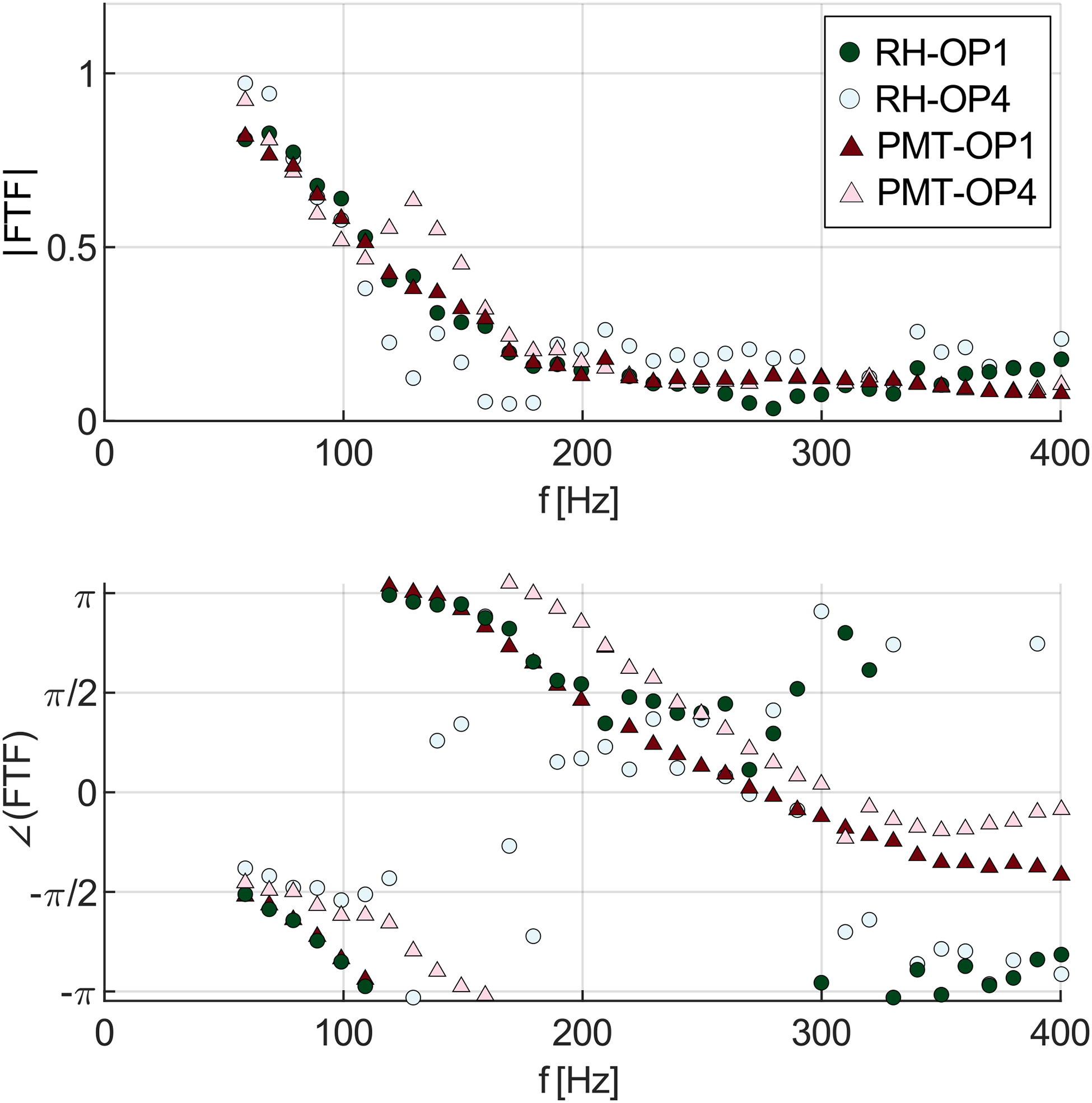
Figure 12 shows FTFs measured with the pure acoustic RH and the hybrid PMT method for the most reactive point OP1 and the least reactive point OP4. For the latter, the highest deviation between RH-OP4 and PMT-OP4 is observed in the frequency range of $f=120-150\mathrm{Hz}$ . Where RH-OP4 shows a local minimum, PMT-OP4 has a local maximum at $f=130\mathrm{Hz}$ . For the phase slopes RH-OP4 already starts with high scattering from $f=120\mathrm{Hz}$ on where PMT-OP4 still shows constant behavior. OP4 is the leanest operation point and the primary zone is operated with ${\varphi }_{\mathrm{pz}}=1.11$ . Beyond this, only a small amount of heat is released in the secondary zone resulting in a very small temperature increase due to combustion. These preconditions do not favor BFTM and BTM measurements, leading to high scattering and uncertainty in the RH-OP4 calculation. Conversely, for the most reactive point OP1, both FTFs fall on top of each other till the phase of RH-OP1 starts to deviate as for OP2 for frequencies higher $f=200\mathrm{Hz}$ .

Figure 12.

Flame transfer functions for operating point OP1 and OP4, pure acoustic ${\mathrm{FTF}}_{\mathrm{RH}}$ (greenish circles) compared with hybrid ${\mathrm{FTF}}_{\mathrm{PMT}}$ (reddish triangles); upper: amplitude of the FTFs; lower: phase angle of the FTFs.

Comparing the phase of OP1 and OP4 a steeper slope is found for the fuel rich OP1 and a shallower for OP4. An explanation can be found via the time delay $\tau =\phi /2\pi f=L_f/u_c$ of each OP. In particular we realize, that the process of radially inward entrainment of ambient fluid is connected with the equivalent radially outward transport of jet fluid in the shear layer by the shear layer turbulence. When the stoichiometric amount of air for the primary mass flow rate $l_{min,p}{\dot{m}}_p$ has been entrained, the flame length $L_F$ is reached. As a consequence the flame length changes, with a larger flame for richer OPs than for leaner ones ( $L_{F,OP1}>L_{F,OP4}$ ). This is visualized in the lower right in Figure 13 in terms of flame center of gravity $x_{\mathrm{COG}}$ . The convective transport velocity $u_c$ is a function of the jet mass fraction and the jet velocity and decreases for leaner operational points ( $u_{c,OP1}>u_{c,OP4}$ ). With a larger change in flame length than convective transport velocity ( $\mathrm{d}{L}_f>\mathrm{d}{u}_c$ ) the time delay $\tau$ decreases towards leaner operational points ( ${\tau }_{OP1}>{\tau }_{OP4}$ ). One ends up with ${\phi }_{OP1}<{\phi }_{OP4}$ which is reflected by the measurement data and shown with the phase slopes in the lower part of Figure 12. A detailed explanation of the physical model used for the estimation of the flame length, convective transport velocity and time delay $\tau$ is supplied in the appendix.

Figure 13.

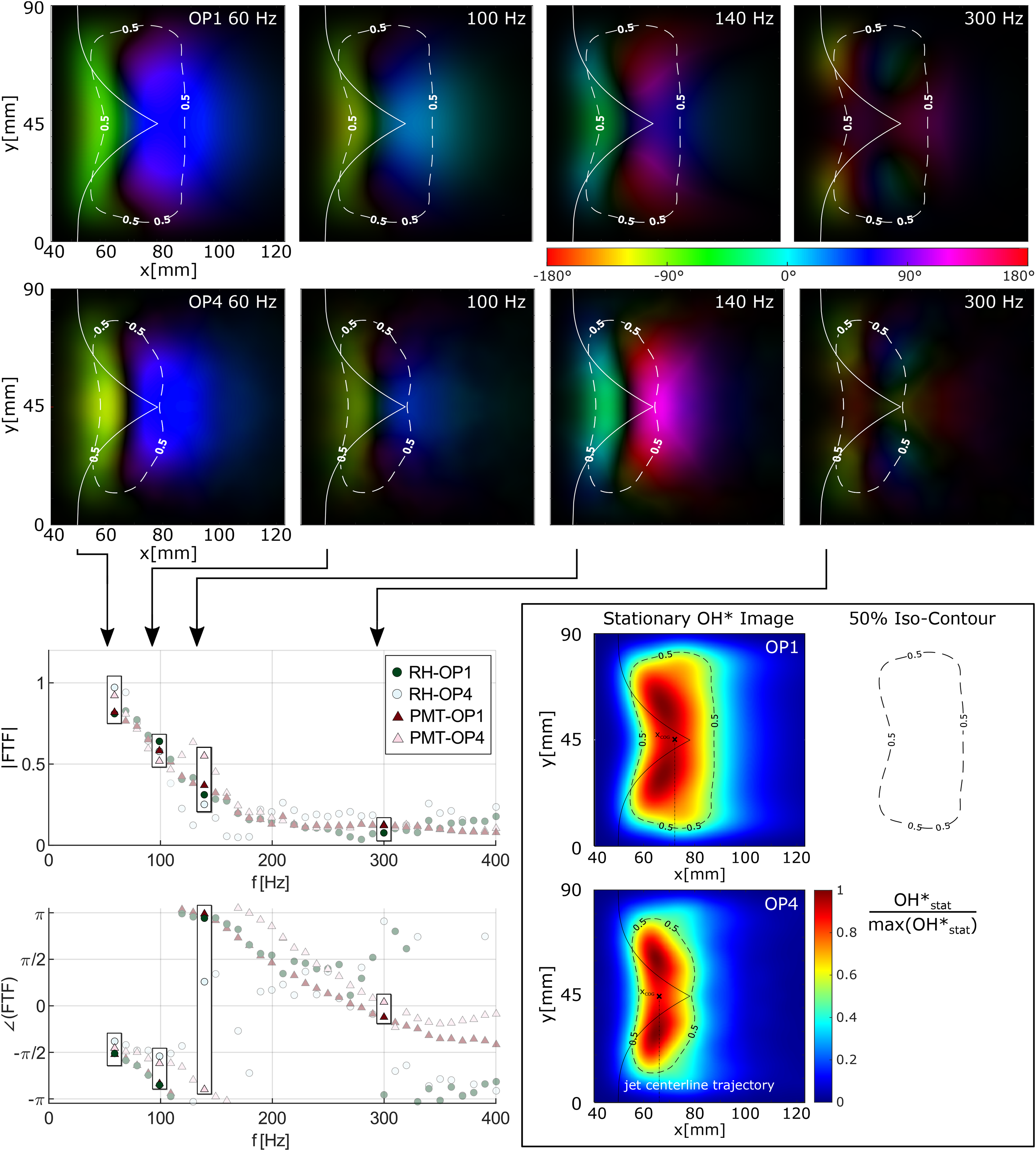
Upper center: comparison of amplitude weighted phase images for the most (OP1) and least (OP4) reactive operation point for selected frequencies; lower left: FTF of OP1 and OP4; lower right: stationary images of the ${\text{OH}}^{*}$ intensity depicting the changes in flame length with the flame center of gravity $x_{\mathrm{COG}}$ for the operation points with the position of the $50\text{\%}$ isocontour and the jet center-line trajectory.

Flame images

Figure 13 shows the normalized time-averaged ${\text{OH}}^{*}$ -intensity distribution images for OP1 and OP4 in the lower right. Both images were normalized by their individual maximum values. A normalization with the overall maximum value was not feasible since ${\mathrm{O}{\mathrm{H}}^{*}}_{\max ,\mathrm{OP}1}$ is several orders of magnitude greater than the least reactive point ${\mathrm{O}{\mathrm{H}}^{*}}_{\max ,\mathrm{OP}4}$ . Additionally, the $50\text{\%}$ ${\text{OH}}^{*}$ -intensity isocontour of the individual image, the flame center of gravity $x_{\mathrm{COG}}$ as a measure of the flame length and the analytically estimated jet center-line trajectory for the upper and lower mixing holes entering the combustion chamber at an axial position of $x=50\mathrm{mm}$ are included. The jet center-line trajectories are only plotted until both reach their maximum penetration depth at the combustor center-line of $y_{\max }=45\mathrm{mm}$ . From the stationary images it can be seen that flame shape in both cases is broadly similar and the ${\text{OH}}^{*}$ distribution can be explained with the JIC theory. The jets entering the combustion chamber immediately start to bend due to the moderate momentum flux ratio $J$ . Afterwards, the jets are distorted from the initial circular shape to a rising kidney shape leading to the characteristic counter-rotating vortex pair (CVP) on the leeward side of the jet.^26–28 Heat release begins at the windward side of the jet root in regions of low scalar dissipation an moderate shear stress. Due to quenching and high strain, no ${\text{OH}}^{*}$ -radicals are found in this region. Combustion expands around the jet, merges on the leeward side and travels along the jet direction into the CVP. ²⁹ The CVP in combination with the opposing jet configuration is favorable for the entrainment and the heat release on the leeward side. In the inner region of the CVP, low scalar dissipation rates, moderate shear and low flow velocity lead to longer residence time and high heat release. ²³ This is where the peak of the ${\text{OH}}^{*}$ -intensity is located for all operating points.

Comparing the flame length of OP1 and OP4 confirms the findings from the FTF phase slopes shown again in the lower left of Figure 13. The convective time delays change with respect to the different flame lengths. The larger flame of OP1 compared with OP4 results in a steeper phase slope for OP1 and a shallower slope for OP4.

The upper part of Figure 13 shows the amplitude weighted phase images of OP1 in row one and of OP4 in row two. In order to verify the phase slopes of the two operation points, the forcing frequency was set to $f=60\mathrm{Hz}$ in a case where the phase values nearly match, and to $f=100,140$ and $300\mathrm{Hz}$ in the other cases, where a stronger deviation is observed. The stationary $50\text{\%}$ ${\text{OH}}^{*}$ -intensity isocontour and the jet center-line trajectory are added to all images as a reference. For the lowest frequency, OP1 shows an axial phase shift from $-{45}^{\circ }$ to $+{45}^{\circ }$ (green to blue), while the regions of highest activity seem to be in the upstream and downstream edges of the flame. The latter observation also applies to OP4 at $f=60\mathrm{Hz}$ but with a difference in the axial phase shift from $-{90}^{\circ }$ to $+{45}^{\circ }$ (yellowish to blue). The same applies for $f=100\mathrm{Hz}$ . Again OP1 shows a more colorful decay from $-{90}^{\circ }$ to $+0^{\circ }$ in axial direction compared to $-{120}^{\circ }$ to $+{30}^{\circ }$ of OP4 with the position of highest activity staying constant at the upstream and downstream edges of the flame. The highest deviation is found at $f=140\mathrm{Hz}$ . At this frequency, OP1 displays the full color spectrum from $-{180}^{\circ }$ to $+{180}^{\circ }$ unlike OP4. In addition to the change in the absolute phase values with increasing frequency, an increase in the relative phase distribution over the flame can be discerned. As for the change in phase from the FTFs, the reason for this is the convective transport, which increases with increasing frequency.

Finally, the FTF amplitude and the brightness of the amplitude weighted phase images in the upper part of Figure 13 are compared. For OP1, the amplitude starts with its global maximum of $|{\mathrm{FTF}}_{\mathrm{PMT}-\mathrm{OP}1}|=0.80$ at $f=60\mathrm{Hz}$ . With increasing frequency, the amplitude falls to a value of $|{\mathrm{FTF}}_{\mathrm{PMT}-\mathrm{OP}1}|=0.14$ at $f=180\mathrm{Hz}$ . From there, the amplitude stays almost constant at its low value for all higher frequencies. The first image on the left in the upper row of Figure 13 at $f=60\mathrm{Hz}$ is the brightest, and corresponds to the global maximum. With increasing frequency in the images to the right, the brightness decreases towards the minimum seen in the image on the far right hand side at $f=300\mathrm{Hz}$ . It is the darkest image (almost black) indicating a low amplitude and thus low amplitude values. For OP4 in the second row, the overall trend remains the same. By comparing the images at $f=100\mathrm{Hz}$ and $f=140\mathrm{Hz}$ a brighter image for the latter is found. This is in line with the increase in the FTF amplitude of OP4 from $100\mathrm{Hz}\to 140\mathrm{Hz}$ as seen in the PMT-OP4 plot. For all images and measured FTFs a good agreement is found. Both show higher interaction between the flame and acoustics in the low frequency range and are not prone to frequencies above $f=200\mathrm{Hz}$ . Consequently, the determination of the frequency range with high interaction between flame and acoustic can also be done via the amplitude weighted phase images.

Conclusions and outlook

In the present paper the setup for thermoacoustic investigations of the lean secondary zone was explained in detail. The lean secondary zone was investigated in terms of acoustic velocity fluctuations coming from the end of the primary zone. Acoustically stiff mixing ports were ensured that no thermoacoustic interaction between the crossflow and the jet generate additional flame dynamics. This reduced the complexity from the former 3-port configuration to a 2-port system. Flame-transfer-functions (FTF) were recorded showing the influence of velocity fluctuations from the primary zone on the thermoacoustic behavior of the lean zone. By systematic comparisons between pure acoustically determined FTFs from the Multi-Microphone-Method (MMM) and Rankine-Hugoniot (RH) equation and FTFs of a hybrid approach with a photomultiplier tube (PMT) using the ${\text{OH}}^{*}$ chemiluminescence as a measure for the heat release, the following conclusions could be drawn:

Within the investigated operating range under constant thermal power, the flame of the lean secondary zone only reacts to acoustic velocity fluctuations with heat release fluctuations in the low frequency range of $f=60-180\mathrm{Hz}$ and shows a clear low pass behavior.

For higher frequencies the RH method shows high scattering due to bad signal-to-noise ratio between the BTM and BFTM measurements. Here the PMT methods excels and reproduces high quality trends for all operating points.

The FTFs measured with pure acoustic RH (baseline) and the ones from the PMT match in terms of their amplitude and phase values very well. ${\text{OH}}^{*}$ seems to work good as a measure for the heat release fluctuations for the investigated inverse diffusion flame presented in this work.

The amplitude weighted phase images showed a change in absolute and relative phase values over the flame length and changes of the amplitude with higher amplitude at low frequencies and indicating lower amplitude with increasing frequency. This is in line with the finding of the FTFs.

For future work it is planed to extend the operating range to operation points with constant pressure drop which is closer to industrial applications. Since the ${\text{OH}}^{*}$ chemiluminescence data with the PMT and HS camera setup gave good results, those methods will be used in addition to the RH method for future determination of flame dynamics and the FTF in the lean secondary zone.