Autoignition flame transfer matrix: Analytical model versus large eddy simulations

Abstract

Modern gas turbines need to fulfil increasingly stringent emission targets on the one hand and exhibit outstanding operational and fuel flexibility on the other. Ansaldo Energia GT26 and GT36 gas turbine models address these requirements by employing a combustion system in which two lean premixed combustors are arranged in series. Due to the high inlet temperatures from the first stage, the second combustor stage predominantly relies on autoignition for flame stabilization. In this paper, the response of autoignition flames to temperature, pressure and velocity excitations is investigated. The gas turbine combustor geometry is represented by a backward-facing step. Based on the conservation equations an analytical model is derived by solving the linearized Rankine-Hugoniot conditions. This is a commonly used analytical approach to describe the relation of thermodynamic quantities up- and downstream of a propagation stabilized flame. In particular, the linearized Rankine-Hugoniot jump conditions are derived taking into account the presence of a moving discontinuity as well as upstream entropy inhomogeneities. The unsteady heat release rate of the flame is modelled as a linear superposition of flame transfer functions, accounting for velocity, pressure, and entropy disturbances, respectively. This results in a 3 $\times$ 3 flame transfer matrix relating both primitive acoustic variables and the temperature fluctuations across the flame. The obtained analytical expression is compared to large eddy simulations with excellent agreement. A discussion about the contribution of the single terms to the modelling effort is provided, with a focus on autoignition flames.

Introduction

The energy landscape is in the midst of a profound transformation. In order to fulfill the goals of the Paris Agreement, power generation needs to be decarbonized. This will result in a fast increasing share of variable renewable power, which has to be balanced by technologies that allow for dispatchable power generation able to flexibly respond to a varying load demand and renewables production. Especially, in so-called Power-to-X-to-Power schemes, gas turbines are predestined to take over this role.

In order to guarantee best-in-class operational and fuel flexibility with ultra-low emissions, Ansaldo Energia GT26 and GT36 feature a sequential combustor architecture. ¹ Sequential combustion systems consist of two combustor stages. The first lean-premix stage is mainly aerodynamically stabilized (vortex breakdown, flame propagation), whereas flame stabilization in the second stage relies predominantly on autoignition. For both flames, fuel and oxidant are premixed and for ease of notation they are in the following referred to as propagation and autoignition flames, respectively.^2,1 In order to assess the thermoacoustic characteristics of a combustion system, a common approach is to make use of the network modelling approach. The complex system is divided into multiple subsystems for which (thermo-)acoustic transfer functions can be derived. ³ Usually, one of these subsystems contains the flame response to acoustic fluctuations. This so-called flame transfer matrix (FTM) relates fluctuating quantities up- and downstream of the flame. For propagation stabilized lean natural gas flames, the FTM can be conveniently measured under atmospheric conditions due the fact that the turbulent flame speed is only weakly pressure dependent.^4,5For autoignition stabilized flames, this straightforward approach is not possible. This is due to the fact that flame stabilization, autoignition delay time, and reaction rates strongly depend on the mean pressure level and the flame dynamics are sensitive to oscillations of temperature and pressure. An alternative to measuring FTM under full engine pressure is to perform unsteady large eddy simulations (LES) coupled with system identification (SI) techniques. This methodology has been introduced for propagation stabilized flames^6,7 and has been recently used to characterize reheat flame dynamics.^8,9 Lately, research efforts on autoignition flame thermoacoustics for gas turbine applications have increased. Research at Ansaldo Energia of Bothien and co-workers focuses on flame transfer functions and matrices.^8–11 Schulz and Noiray^12,13 as well as Aditya et al. ¹⁴ and Gruber et al. ¹⁵ investigate the occurrence of propagation and autoignition stabilized regimes of reheat flames. In contrast to propagation stabilized flames, only a few studies on analytical modelling approaches for autoignition flame acoustics exist.^16–18 Although the characterization of autoignition flame dynamics by combined LES/SI approaches shows very promising results, it comes with the drawback that retrieving the FTM for the whole engine operating regime and different burner variants in new development programmes is far too time consuming. In this paper, we therefore focus on deriving an analytic expression for the dynamics of autoignition stabilized flames starting from the general conservation equations, which is then benchmarked with LES/SI results. For this purpose, the Rankine-Hugoniot jump conditions relating fluctuating quantities up- and downstream of the flame are derived. Chu ¹⁹ was the first to derive these jump conditions across a flame front in 1953. Additionally, analytical models for autoignition flame transfer functions (FTFs) to acoustic and entropic disturbances^17,11 are incorporated in the FTM modelling, resulting in a closed-form expression directly comparable to LES/SI results.

This work is an extension of two previous research papers,^8,20 revisited and deepened with the inclusion of new material from recent research on autoignition flames.^11,18

The Rankine-Hugoniot jump conditions

The Rankine-Hugoniot conditions are one-dimensional integral conditions describing mass, momentum and energy conservation across a discontinuity – in the present case a flame. This discontinuity can be modelled to be at rest or in motion. As was for example shown in a recent publication, ¹⁰ in reheat flames the flame front position is highly responsive to the modification of the autoignition delay time of the unburnt mixture. This in turn is influenced by the excitation applied at the system boundary. Including this phenomenon in the model is crucial for autoignition flames.

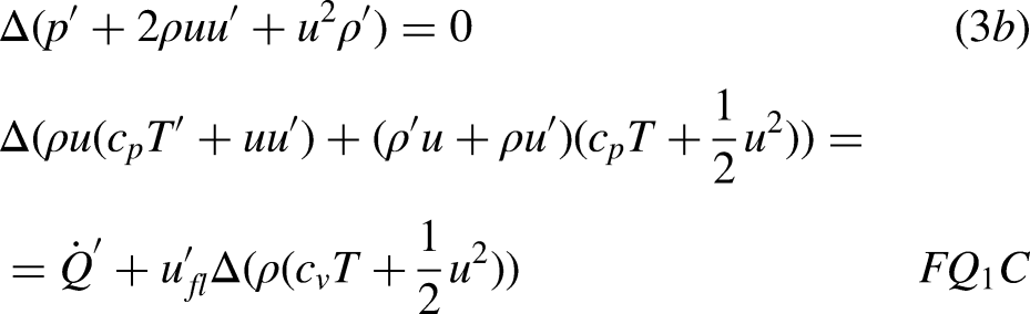
The following integral conservation equations relate the up- and downstream quantities across a flame front^19,21:

$$\mathrm{\Delta }(\rho u)=u_{fl}\mathrm{\Delta }\rho$$

(1a)

$$\mathrm{\Delta }(\rho u^2+p)=u_{fl}\mathrm{\Delta }(\rho u)$$

(1b)

$$\mathrm{\Delta }(\rho u(c_{p}T+\frac{1}{2}{u}^2))=u_{fl}\mathrm{\Delta }(\rho (c_{v}T+\frac{1}{2}{u}^2))+\dot{Q}$$

(1c)

where $p$ is the pressure, $u$ the velocity, $\rho$ the density, $T$ the temperature, $\dot{Q}$ the flame heat release rate per unit area, and $u_{fl}$ the flame location velocity. The coefficients $c_p$ and $c_v$ denote the mixture specific heat capacity, at constant pressure and at constant volume respectively. The subscripts denote states up- ( $1$ ) and downstream ( $2$ ) of the flame and the symbol $\mathrm{\Delta }$ stands for the difference between quantities in $2$ and in $1$ , e.g. $\mathrm{\Delta }p=p_2-p_1$ . Closure of the set of Eqs. (1) is done via the ideal gas law, $p_i={\rho }_{i}R{T}_i$ with $\text{i=1, 2}$ . Together with the system given by Eqs. (1) this is a nonlinear algebraic system of four equations for the four unknown downstream quantities $u_2,p_2,{\rho }_2,T_2$ .

Linearization of the conservation equations

Acoustic disturbances are small fluctuations with respect to the mean value. Each physical quantity can be written as a sum of a mean value and an acoustic fluctuation as: $\phi (x,t)=\overline{\phi }+{\phi }^{\prime }(x,t)$ , where $\overline{(\cdot )}$ denotes the mean quantity and $(\cdot {)}^{\prime }$ the fluctuating term. $\phi$ is a general flow variable, e.g., pressure $p$ , velocity $u$ , density $\rho$ .

If the acoustic amplitudes are sufficiently small, ${\phi }^{\prime }\ll \overline{\phi }$ , the acoustic equations may be derived by a first-order approximation of the conservation equations neglecting nonlinear second- or higher-order effects ( ${\phi }^{\prime 2}<<{\phi }^{\prime }$ ). Linearization of Eqs. (1) then yields the following two sets of equations, one for the mean parts

$${\rho }_2{u}_2={\rho }_1{u}_1$$

(2a)

$${\rho }_2{u}_2^2+p_2={\rho }_1{u}_1^2+p_1$$

(2b)

$${\rho }_2{u}_2(c_p{T}_2+u_2^2/2)={\rho }_1{u}_1(c_p{T}_1+u_1^2/2)+\dot{Q}$$

(2c)

$$p_2/({\rho }_2{T}_2)=p_1/({\rho }_1{T}_1)=R$$

(2d)

and one for the fluctuating ones

$$\mathrm{\Delta }({\rho }^{\prime }u+\rho u^{\prime })=u_{fl}^{\prime }\mathrm{\Delta }\rho$$

(3a)

$$\begin{array}{rl}(3b)& & \mathrm{\Delta }(p^{\prime }+2\rho u{u}^{\prime }+u^2{\rho }^{\prime })=0& \mathrm{\Delta }(\rho u(c_p{T}^{\prime }+u{u}^{\prime })+({\rho }^{\prime }u+\rho u^{\prime })(c_{p}T+\frac{1}{2}{u}^2))=\dots \\ F{Q}_{1}C& & \cdots ={\dot{Q}}^{\prime }+u_{fl}^{\prime }\mathrm{\Delta }(\rho (c_{v}T+\frac{1}{2}{u}^2))\end{array}$$

$$p_2^{\prime }/p_2={\rho }_2^{\prime }/{\rho }_2+T_2^{\prime }/T_2,$$

(3c)

where for ease of notation here and in the following the overbar is dropped. It is also assumed that the mean flame velocity is zero, i.e., $u_{fl}=0$ , due to the fact that the excitations of the inlet parameters exhibit zero mean value.

Solution for the mean quantities

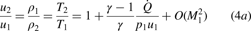
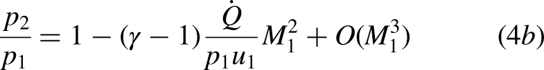
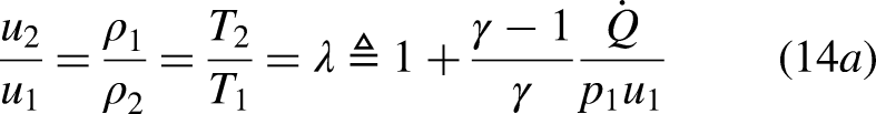
First, we focus exclusively on the mean quantities, given in Eqs. (2). These are four nonlinear coupled equations in the unknowns $u_2,p_2,{\rho }_2,T_2$ . The system can be solved analytically and the solution expanded in the Mach number^19,21:

$$\frac{u_2}{u_1}=\frac{{\rho }_1}{{\rho }_2}=\frac{T_2}{T_1}=1+\frac{\gamma -1}{\gamma }\frac{\dot{Q}}{p_1{u}_1}+O(M_1^2)$$

(4a)

$$\frac{p_2}{p_1}=1-(\gamma -1)\frac{\dot{Q}}{p_1{u}_1}{M}_1^2+O(M_1^3)$$

(4b)

Interestingly, these relations would also hold for the general variables $u(x,t),p(x,t),\rho (x,t),T(x,t)$ and not only for their mean values if a problem without moving discontinuity would have been considered.

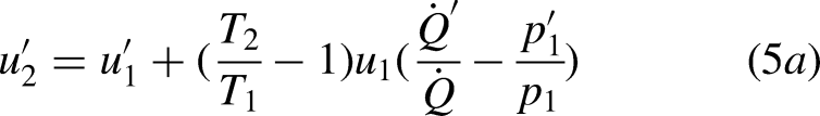
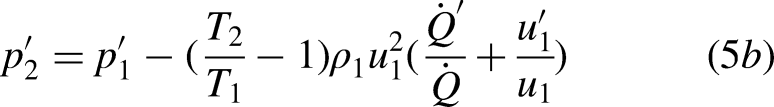
Linearization of Eqs. (4) is common^22,6 and yields:

$$u_2^{\prime }=u_1^{\prime }+(\frac{T_2}{T_1}-1)u_1(\frac{{\dot{Q}}^{\prime }}{\dot{Q}}-\frac{p_1^{\prime }}{p_1})$$

(5a)

$$p_2^{\prime }=p_1^{\prime }-(\frac{T_2}{T_1}-1){\rho }_1{u}_1^2(\frac{{\dot{Q}}^{\prime }}{\dot{Q}}+\frac{u_1^{\prime }}{u_1})$$

(5b)

$$T_2^{\prime }=T_1^{\prime }+(\frac{T_2}{T_1}-1)T_1(\frac{{\dot{Q}}^{\prime }}{\dot{Q}}+\frac{T_1^{\prime }}{T_1}-\frac{p_1^{\prime }}{p_1}-\frac{u_1^{\prime }}{u_1})$$

(5c)

Since in the current framework the flame is changing its axial location due to the ignition delay time dependence on temperature, Eqs. (5) are not valid and need to be derived with $u_{fl}^{\prime }\ne 0$ . In the Discussion section we will elaborate on the reason why Eq. (5) are not suitable to study autoignition flames.

Solution for the fluctuating quantities

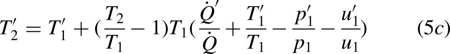
Equations (3) for the fluctuating quantities are linear and can be recast in a matrix form:

$$\begin{array}{rl}& \left[\begin{array}{ccc}\gamma M_1\frac{c_1}{c_2}& \frac{u_1}{u_2}& -\gamma M_1\frac{c_1}{c_2}\\ \frac{c_1}{c_2}\frac{p_2}{p_1}+\gamma M_1{M}_2& 2M_1& -\gamma M_1{M}_2\\ 0& \gamma M_1^2\frac{u_2}{u_1}& \frac{{\gamma }^2}{\gamma -1}{M}_1\frac{c_2}{c_1}\end{array}\right]\left[\begin{array}{c}\frac{p_2^{\prime }}{{\rho }_2{c}_2}\\ u_2^{\prime }\\ \frac{R{T}_2^{\prime }}{c_2}\end{array}\right]=\cdots \\ & \left[\begin{array}{cc}\gamma M_1& 1-\gamma M_1\\ 1+\gamma M_1^2& 2M_1& -\gamma M_1^2\\ -\tilde{\dot{Q}}\gamma M_1& \gamma M_1^2-\tilde{\dot{Q}}& \frac{{\gamma }^2}{\gamma -1}{M}_1+\tilde{\dot{Q}}\gamma M_1\end{array}\right]\left[\begin{array}{c}\frac{p_1^{\prime }}{{\rho }_1{c}_1}\\ u_1^{\prime }\\ \frac{R{T}_1^{\prime }}{c_1}\end{array}\right]+\cdots \\ & & \left[\begin{array}{c}0\\ 0\\ \frac{\dot{Q}}{u_1{p}_1}\end{array}\right]u_1\frac{{\dot{Q}}^{\prime }}{\dot{Q}}+\left[\begin{array}{c}\frac{u_1}{u_2}-1\\ 0\\ 1-\frac{p_2}{p_1}+\tilde{\dot{Q}}\end{array}\right]u_{fl}^{\prime },\end{array}$$

(6)

where $\tilde{Q}=\frac{\dot{Q}}{p_1{u}_1}$ and use has been made of the speed of sound $c^2=\gamma p/\rho$ and of the Mach number $M\triangleq u/c$ . The independent variables $p^{\prime }$ , $u^{\prime }$ and $T^{\prime }$ have been normalized so that they have the dimension of a velocity. Equation (6) provides the downstream fluctuating quantities as function of the upstream ones. We focus now on the last two summands and try to express ${\dot{Q}}^{\prime }$ and $u_{fl}^{\prime }$ as functions of the upstream quantities $p_1^{\prime }/(c_1{\rho }_1)$ , $R{T}_1^{\prime }/c_1$ and $u_1^{\prime }$ .

Representation of the unsteady heat release rate

It is assumed that the individual contributions of pressure, velocity and temperature fluctuations on the unsteady heat release rate can be linearly superposed and that they are related to the relative heat release rate fluctuations by the frequency dependent flame transfer functions.

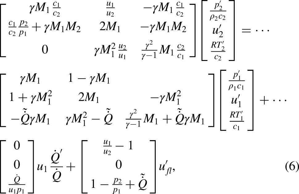
Bothien et al. ⁸ showed that for the linear case relative heat release rate fluctuations can be expressed as

$$\begin{array}{rl}\frac{{\dot{Q}}^{\prime }}{\dot{Q}}& =F_p\frac{p_1^{\prime }}{p_1}+F_u\frac{u_1^{\prime }}{u_1}+F_T\frac{T_1^{\prime }}{T_1}=\cdots \\ & \left[\begin{array}{ccc}\frac{\gamma }{c_1}{F}_p& \frac{1}{u_1}{F}_u& \frac{\gamma }{c_1}{F}_T\end{array}\right]\left[\begin{array}{c}\frac{p_1^{\prime }}{{\rho }_1{c}_1}\\ u_1^{\prime }\\ \frac{R{T}_1^{\prime }}{c_1}\end{array}\right],\end{array}$$

(7)

where $F_p$ , $F_u$ , and $F_T$ are the complex-valued, frequency dependent flame transfer functions of the single contributions. This approach based on the superposition of contributions is particularly useful to model the problem and understand the physical mechanisms involved. The key point to justify this methodology is the linearity assumption, which has been carefully validated in a previous work, ⁸ showing that the superposition principle is applicable as long as we consider small temperature fluctuations.

Analytic flame transfer function models

The analytical formulations for the autoignition flame transfer functions are obtained by merging the model of Zellhuber et al. ¹⁷ for acoustic fluctuations with the model of Gant et al. ¹¹ for entropic disturbances. The unsteady heat release rate can then be expressed in the frequency domain as ¹⁸ :

$$\begin{array}{rl}\frac{{\dot{Q}}^{\prime }}{\overline{\dot{Q}}}=& (\frac{u_1^{\prime }}{u_1}+\frac{1}{\gamma }\frac{p_1^{\prime }}{p_1}-\frac{s_1^{\prime }}{c_p})e^{-i\omega \tau }{e}^{-{\omega }^2{\sigma }^2/2}-{\phi }_p\frac{p_1^{\prime }}{p_1}{e}^{-i\omega \tau }{e}^{-{\omega }^2{\sigma }^2/2}\\ +& {\phi }_p\frac{p^{\prime }(x_{fl})}{p_1}{e}^{-{\omega }^2{\sigma }^2/2}-\tau {\phi }_T\omega T_{1}i{e}^{-i\omega \tau }{e}^{-{\omega }^2{\sigma }^2/2}\frac{s_1^{\prime }}{c_p}\end{array}$$

(8)

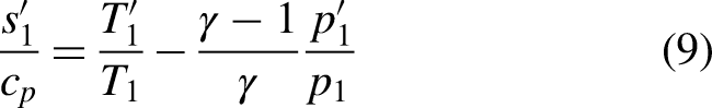
where ${\phi }_p$ and ${\phi }_T$ are autoignition pressure and temperature sensitivity factors,^17,11 $\tau$ is the mean ignition delay time, $\sigma$ is a measure of the flame thickness, $p^{\prime }(x_{fl})$ is the acoustic pressure fluctuation at the flame location, and $s_1^{\prime }$ is an entropic fluctuation:

$$\frac{s_1^{\prime }}{c_p}=\frac{T_1^{\prime }}{T_1}-\frac{\gamma -1}{\gamma }\frac{p_1^{\prime }}{p_1}$$

(9)

Four different physical mechanisms are responsible for the unsteady heat release rate:

• $(\frac{u_1^{\prime }}{u_1}+\frac{1}{\gamma }\frac{p_1^{\prime }}{p_1}-\frac{s_1^{\prime }}{c_p})e^{-i\omega \tau }{e}^{-{\omega }^2{\sigma }^2/2}$ are mass flow fluctuations at the location $1$ at the time $t-\tau$ . They are convected to the flame and cause a heat release rate fluctuation at time $t$ .

• $-(\tau {\phi }_T\omega T_{1}i)e^{-i\omega \tau }{e}^{-{\omega }^2{\sigma }^2/2}\frac{s_1^{\prime }}{c_p}$ are entropic fluctuations at the location $1$ at the time $t-\tau$ . They affect the autoignition time of the mixture as it travels downstream towards the flame front.

• $-{\phi }_p\frac{p_1^{\prime }}{p_1}{e}^{-i\omega \tau }{e}^{-{\omega }^2{\sigma }^2/2}$ are pressure waves affecting the reaction progress of the mixture as it travels downstream towards the flame front.

• ${\phi }_p\frac{p^{\prime }(x_{fl})}{p_1}{e}^{-{\omega }^2{\sigma }^2/2}$ are changes of acoustic pressure at the flame location. They have an important effect on the flame response at high frequency.

More details on Eq. (8) and its physical interpretation can be found in the literature.^17,11,18 If the acoustic field is assumed to be compact, $\tau \omega <<1$ (which is valid for the plane wave transfer matrix approach considered here) and for low Mach numbers, $M<<1$ , it can be shown that pressure fluctuations at the flame $x_{fl}$ can be related to those at the location $1$ by $p^{\prime }(x_{fl},t)\approx p^{\prime }(x_1,t)$ . Additionally, using Eq. (9), the flame transfer functions $F_p$ , $F_u$ , and $F_T$ are obtained by comparison of Eq. (8) to Eq. (7):

$$F_p=(\frac{1}{\gamma }-{\phi }_p(1-e^{i\omega \tau }))e^{-i\omega \tau }{e}^{-{\omega }^2{\sigma }^2/2}-\frac{\gamma -1}{\gamma }{F}_T$$

(10a)

$$F_u=e^{-i\omega \tau }{e}^{-{\omega }^2{\sigma }^2/2}$$

(10b)

$$F_T=-(1+\tau {\phi }_T\omega T_{1}i)e^{-i\omega \tau }{e}^{-{\omega }^2{\sigma }^2/2}$$

(10c)

Solution for the moving flame

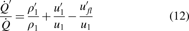
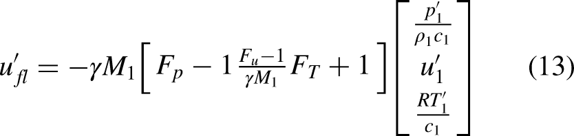
The dependence of $u_{fl}^{\prime }$ on the upstream fluctuations can be expressed conveniently if the flame is assumed to be a thin discontinuity between the unburnt and the burnt mixture. The heat release rate per unit area depends on the amount of fuel crossing the flame front per unit time, i.e., the relative velocity between the flame and the mean flow as well as the density of the fuel and can be written as

$$\dot{Q}={\rho }_1(u_1-u_{fl})\mathrm{\Delta }{h}_F,$$

(11)

where $\mathrm{\Delta }{h}_F$ is the fuel lower heating value. The hypothesis of perfectly premixed mixture allows us to neglect equivalence ratio fluctuations. Linearization of Eq. (11) around the mean condition (with $u_{fl}=0$ as explained above) gives:

$$\frac{{\dot{Q}}^{\prime }}{\dot{Q}}=\frac{{\rho }_1^{\prime }}{{\rho }_1}+\frac{u_1^{\prime }}{u_1}-\frac{u_{fl}^{\prime }}{u_1}$$

(12)

and combination with Eq. (7) yields the expression for the fluctuating flame velocity:

$$u_{fl}^{\prime }=-\gamma M_1\left[\begin{array}{c}{F}_p-1\frac{F_u-1}{\gamma M_1}{F}_T+1\end{array}\right]\left[\begin{array}{c}\frac{p_1^{\prime }}{{\rho }_1{c}_1}\\ u_1^{\prime }\\ \frac{R{T}_1^{\prime }}{c_1}\end{array}\right]$$

(13)

Final expression

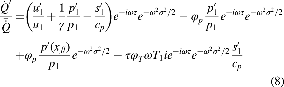
Equation (6) can be expanded inserting Eq. (7) for the unsteady heat release rate, Eq. (13) for the moving flame, and Eq. (10) for the FTFs. For the mean quantities in the matrices in Eq. (6) , a first order approximation of Eqs. (4) yields:

$$\frac{u_2}{u_1}=\frac{{\rho }_1}{{\rho }_2}=\frac{T_2}{T_1}=\lambda \triangleq 1+\frac{\gamma -1}{\gamma }\frac{\dot{Q}}{p_1{u}_1}$$

(14a)

$$\frac{p_2}{p_1}=1$$

(14b)

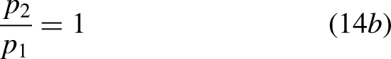
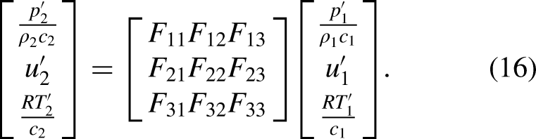
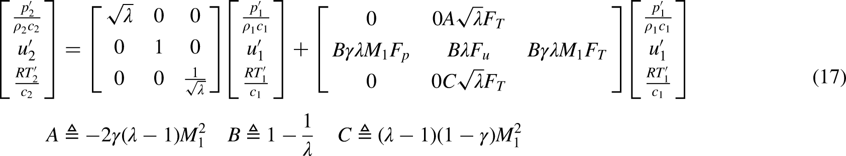
Substituting Eqs. (14) in Eq. (6), inverting the matrix on the left hand side and computing the products we obtain:

$$\begin{array}{rl}\left[\begin{array}{c}\frac{p_2^{\prime }}{{\rho }_2{c}_2}\\ u_2^{\prime }\\ \frac{R{T}_2^{\prime }}{c_2}\end{array}\right]& =[\begin{array}{c}\sqrt{\lambda }+\sqrt{\lambda }\gamma (\lambda -1)M_1^2\\ -\gamma (\lambda -1)M_1+\gamma \lambda (1-\lambda )M_1^3\\ (\gamma -1)\sqrt{\lambda }(\lambda -1)M_1^2\end{array}\dots \\ & \dots \begin{array}{cc}0& 0\\ 1+(1-\gamma )(\lambda -1)M_1^2& 0\\ -\frac{\gamma -1}{\gamma }\frac{\lambda -1}{\sqrt{\lambda }}{M}_1& \frac{1}{\sqrt{\lambda }}\end{array}]\left[\begin{array}{c}\frac{p_1^{\prime }}{{\rho }_1{c}_1}\\ u_1^{\prime }\\ \frac{R{T}_1^{\prime }}{c_1}\end{array}\right]+\\ & +\left[\begin{array}{ccc}A\sqrt{\lambda }{F}_p& A\frac{\sqrt{\lambda }}{\gamma M_1}{F}_u& A\sqrt{\lambda }{F}_T\\ B\gamma \lambda M_1{F}_p& B\lambda F_u& B\gamma \lambda M_1{F}_T\\ C\sqrt{\lambda }{F}_p& C\frac{\sqrt{\lambda }}{\gamma M_1}{F}_u& C\sqrt{\lambda }{F}_T\end{array}\right]\left[\begin{array}{c}\frac{p_1^{\prime }}{{\rho }_1{c}_1}\\ u_1^{\prime }\\ \frac{R{T}_1^{\prime }}{c_1}\end{array}\right]\\ A& \triangleq -2\gamma (\lambda -1)M_1^2\\ B& \triangleq 1-\frac{1}{\lambda }+(\lambda -1)(\gamma +1)M_1^2\\ C& \triangleq (\lambda -1)(1-\gamma )M_1^2\end{array}$$

(15)

where $\lambda$ is defined in Eq. (14a). The first matrix in Eq. (15) represent the static contribution of the flame, whereas the second matrix in Eq. (15) represent the dynamic, frequency-dependent contribution. Each column of the FTM depends on a single element of the flame transfer function, therefore there are no cross dependencies between FTF elements in the FTM. This is to be expected since a linear framework is considered. Equation (15) can be simplified to Eq. (27) given by Chen et al. ²¹ .

Numerical setup

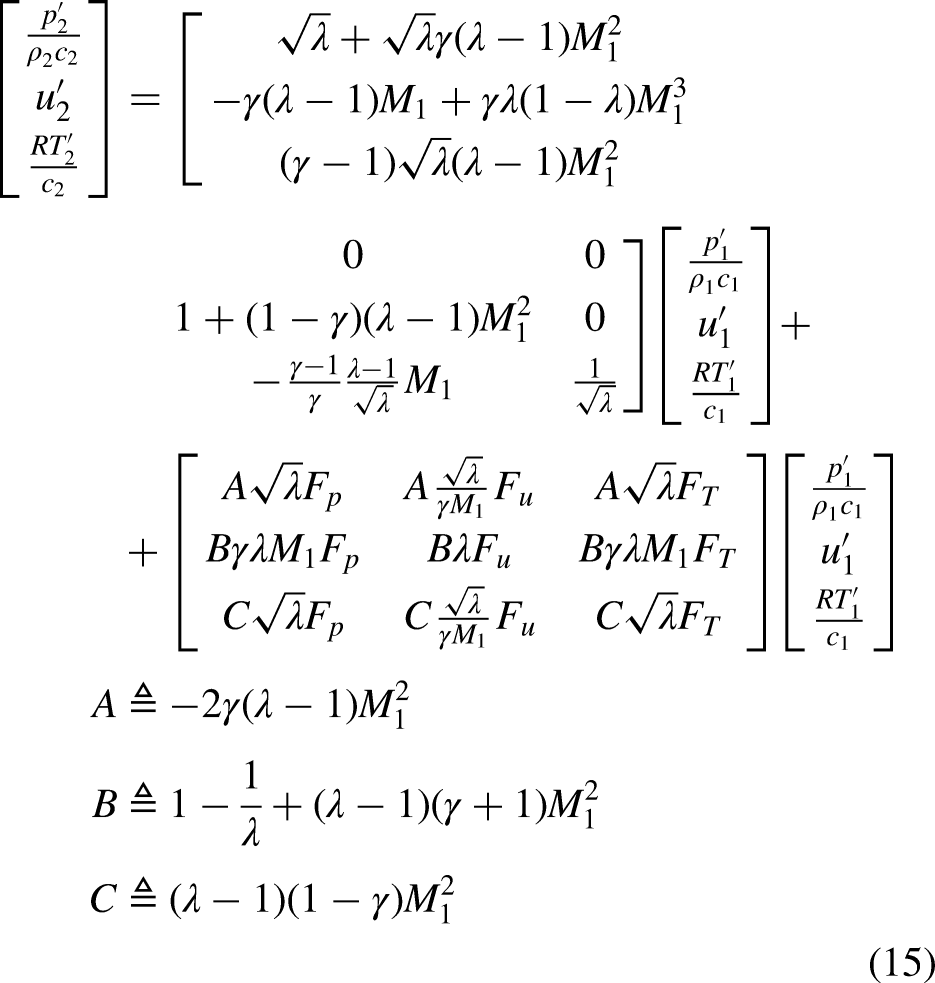
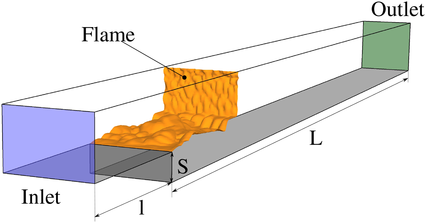
Figure 1 shows the simplified reheat combustor used in this study to benchmark the analytic model described above. This backward-facing step (BFS) geometry has been used by Bothien et al. ⁸ to derive the 3 $\times$ 3 flame transfer matrix for an autoignition flame. In the following, the geometry, the numerical set up, the combustion model and the system identification methodology are briefly explained. More detailed information is provided in Ref. ⁸ .

Figure 1.

Backward-facing step used for LES reproduced from Bothien et al. ⁸ .

Perfectly premixed air and methane are injected through the inlet of the domain. On the bottom surface a no-slip boundary condition assures the presence of a boundary layer, whereas periodic boundary conditions are applied on the two side walls. The top surface is a symmetry plane so as to have a closer representation to the realistic geometry with a two-sided BFS. The geometry is meshed with 2.11 million hexahedral cells and the simulations are run on the commercial software ANSYS Fluent v17.0. Turbulence scales larger than the mesh size are computed, whereas the Smagorinsky model with Lilly dynamic procedure is used to model the subgrid-scale. The turbulent Schmidt number is set to 0.7 for scalar flux and for species. The combustion model relies on tabulated chemistry and a progress variable and is particularly suited to study autoignition flames dynamics. ²³ In particular, the reaction kinetics are tabulated and obtained from a 0D homogeneous reactor calculation with detailed chemistry. A composite progress variable is defined and utilized to parametrize the reaction evolution, and all thermo-chemical quantities of interest are tabulated as function of this progress variable and of the mixture fraction. The combustion model solves the transport equations of the progress variable and the mixture fraction and reads the other variables values from the tables, including intermediate species and products. ²³ The chemistry-turbulence interaction is modelled by means of a composition transported filtered density function method based on a Eulerian formulation.

Three compressible simulations are run, exciting the outlet pressure, the inlet temperature and the inlet velocity, respectively. The excitation is provided by forcing at discrete frequencies and in form of a low-pass filtered discrete random binary signal (DRBS), which allows a frequency broadband excitation of the flame. In order to avoid thermoacoustic instabilities, the respective opposite side of the domain that is not excited is set to non-reflecting.

The flame dynamics investigated in this work are assumed to be linear and time-invariant. Hence, the system response is obtained from the sum of the convolutions of its finite impulse responses with their respective input signals. For this, a suitable system identification (SI) method is applied to reconstruct the multi-parameter system from the large eddy simulations. This method is well suited to identify the flame response to broadband input signals while minimizing noise. ⁹ In Ref. ⁸ , the single steps of this procedure are explained in detail, and can be summarized as follows:

Velocity, pressure and temperature signals are extracted at a number of different axial location as time-dependent section-averaged quantities. Each signal is shifted to a reference location applying a characteristic-based filter (CBF). ²⁴ This methodology is able to filter out turbulent noise and retain only the meaningful signal information.

The flame is assumed to behave as a linear time invariant system. The inputs to this system are the upstream velocity, pressure and temperature signals, the output is the volume-integrated heat release rate. The finite impulse responses (FIR) of the system are calculated from its input and output information using the Wiener-Hopf equation. ⁶ The FIR transformed in the frequency domain provide the flame transfer functions $F_u$ , $F_p$ and $F_T$ , for the velocity, pressure and temperature respectively.

To identify the FTM the same system identification procedure is applied, considering in this case as output signals the downstream velocity, pressure and temperature fluctuations. Nine frequency dependent functions $F_{ij}$ are obtained, relating up- to downstream fluctuations:

$$\left[\begin{array}{c}\frac{p_2^{\prime }}{{\rho }_2{c}_2}\\ u_2^{\prime }\\ \frac{R{T}_2^{\prime }}{c_2}\end{array}\right]=\left[\begin{array}{c}{F}_{11}{F}_{12}{F}_{13}\\ F_{21}{F}_{22}{F}_{23}\\ F_{31}{F}_{32}{F}_{33}\end{array}\right]\left[\begin{array}{c}\frac{p_1^{\prime }}{{\rho }_1{c}_1}\\ u_1^{\prime }\\ \frac{R{T}_1^{\prime }}{c_1}\end{array}\right].$$

(16)

Discussion

Flame transfer functions

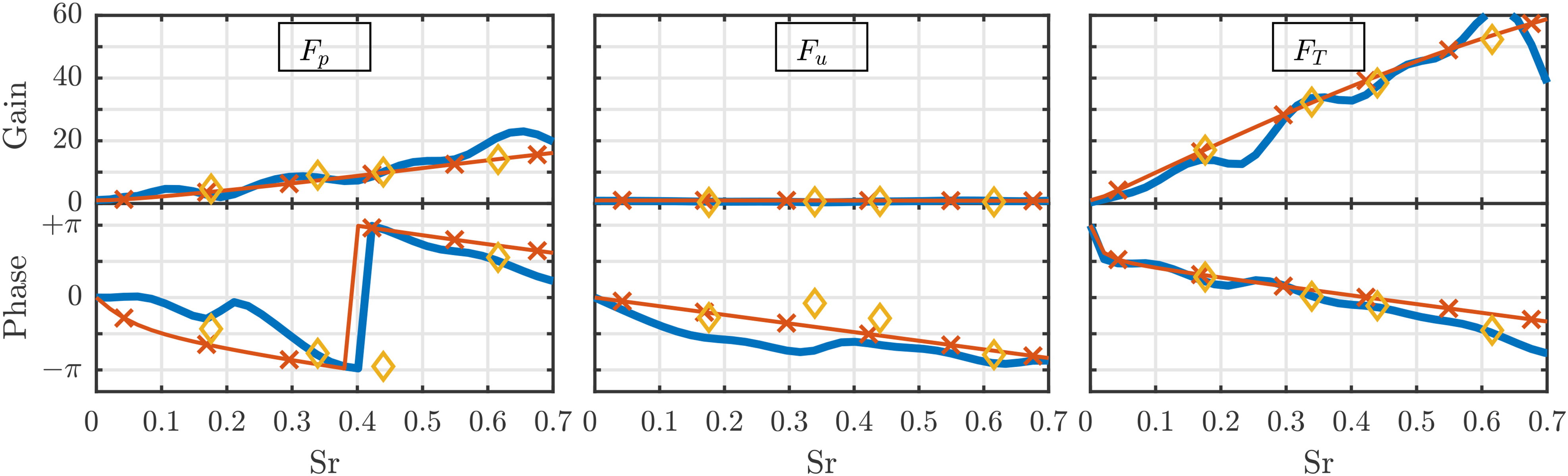
In Figure 2, the individual flame transfer functions are plotted over the Strouhal number, which is defined as $\text{Sr}\triangleq fu/L$ with $L$ being the step height and $u$ the mean flow velocity.

Figure 2.

Individual flame transfer functions of the BFS autoignition flame. LES/SI result: solid blue, LES discrete forcing: yellow diamonds, analytical model of Eqs. (10): red line with crosses.

Comparison of the gains (top row) reveals the importance of pressure and temperature fluctuations on the generation of heat release rate fluctuations for autoignition flames. For example at Sr = 0.33, $|F_p|=10$ and $|F_T|=35$ whereas $|F_u|$ is two orders of magnitude smaller ( $|F_u|=0.3$ ). The fact that temperature fluctuations can play such a large role is due to the exponential dependence of the mixture ignition delay time on temperature. ¹¹ Consequently, the flame position is largely affected and so is the heat release rate fluctuation. ¹⁰ It has to be noted that this effect is very distinct for the BFS configuration studied here since the resulting flame is almost only autoignition stabilized. This can be deduced from the almost vertical flame front in Figure 1 and is due to the very low turbulence levels at the inlet. For a real engine reheat combustor, the contribution of autoignition to the flame stabilization is still larger than the contribution of propagation, as can be deduced for example from the flame shapes shown by Yang et al. ⁹ , but will be significantly less pronounced.

The analytic model (red line with crosses) Eq. (10) is in excellent agreement to the discrete forcing results of the LES (yellow diamonds). Compared to the broadband results (blue, solid), the analytic model is not following the wavy pattern.

Before discussing the flame transfer matrix, an important point needs to be highlighted: the large difference in magnitude among the flame transfer function gains $|F_p|$ , $|F_u|$ and $|F_T|$ in Figure 2 does not necessarily imply a similar large difference in the contribution of pressure, velocity and temperature fluctuations to the heat release rate fluctuations. Otherwise said, even if $|F_u|$ is very small in Figure 2, its contribution to the heat release rate fluctuations ${\dot{Q}}^{\prime }/\dot{Q}$ cannot be neglected. For example, the fact that $|F_p|$ is approximately 30 times larger than $|F_u|$ does not mean that the heat release rate fluctuations ${\dot{Q}}^{\prime }/\dot{Q}$ caused by pressure fluctuations $p_1^{\prime }/p_1$ will be 30 times larger than those caused by velocity fluctuations $u_1^{\prime }/u_1$ . This is because, as shown in the first line of Eq. 7, the heat release rate fluctuation ${\dot{Q}}^{\prime }/\dot{Q}$ is affected also by $p_1^{\prime }/p_1$ and $u_1^{\prime }/u_1$ , and not only by $F_p$ and $F_u$ . Simple order of magnitude calculations ⁸ show that for a typical reheat flame $p_1^{\prime }/p_1\approx 0.1u_1^{\prime }/u_1$ and therefore that velocity fluctuations can significantly impact ${\dot{Q}}^{\prime }/\dot{Q}$ likewise.

Flame transfer matrix

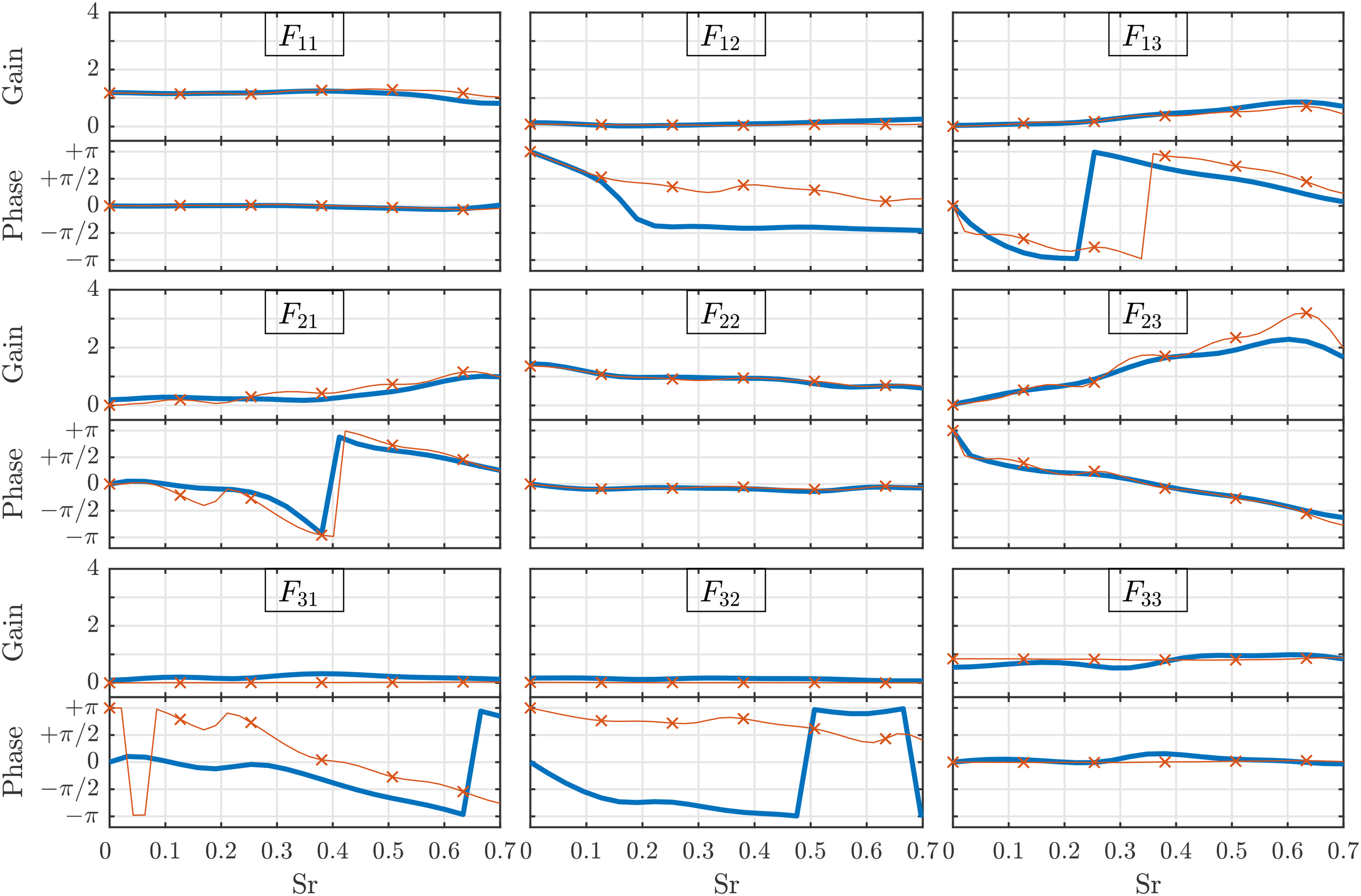
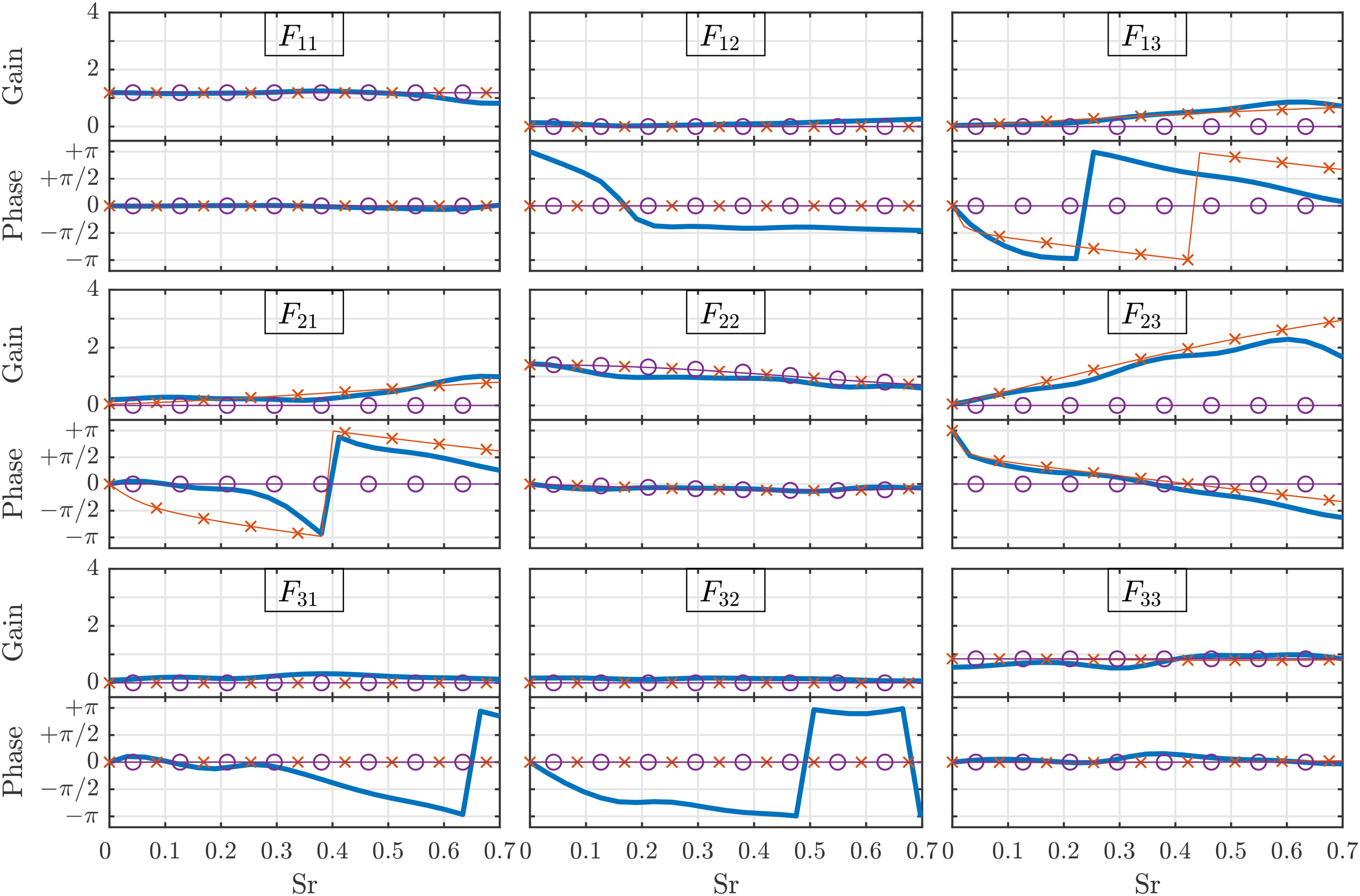
Figure 3 shows the full 3 $\times$ 3 transfer matrix. The LES/SI results (solid blue) are reproduced from Bothien et al. ⁸ . The analytic FTM model given in Eq. (15) is presented in combination with the LES/SI FTFs (red line with crosses). As expected, the model show excellent agreement for all elements. Significant differences are present only in the phase of the elements $F_{12}$ , $F_{31}$ and $F_{32}$ . They are due to the fact that the corresponding gains are small and hence the phase estimation is error-prone. All elements with gains larger than $0.5$ are well reproduced both in gain and in phase confirming the correctness of the assumptions that are made in deriving Eq. (15). Additionally, this excellent match also verifies the consistency of the system identification methodology applied in Ref. ⁸ by means of a completely independent analytical approach. All the elements in the third column of Figure 3 present non-negligible values, showing how incoming temperature fluctuations have a significant impact on the acoustic and entropic fields downstream the flame. This frequency dependent effect is largely function of the autoignition delay time of the reactive mixture and, consequently, of the mean inlet temperature, pressure and of the fuel composition.^17,18,11 In general, variations of these parameters increasing the autoignition delay time, i.e. shifting the flame in a more downstream position, will result in larger gains.

Figure 3.

Flame transfer matrix from LES/SI approach ⁸ (blue, thick line), analytic formulation of Eq. (15) with numeric FTFs (red line with crosses).

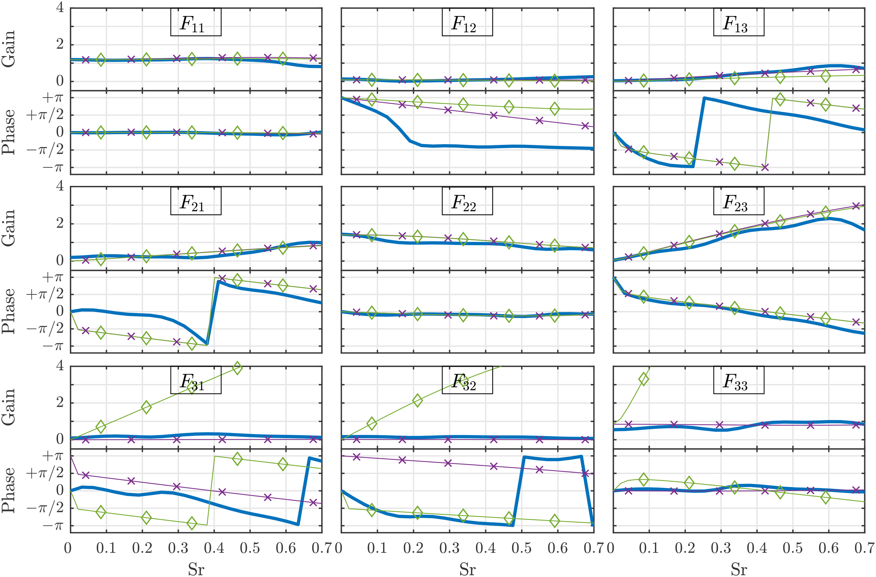
Figure 3 verifies the correctness of the Rankine-Hugoniot relations in Eq. (15) alone. In Figure 4 we aim at verifying the correctness of the Rankine-Hugoniot relations Eq. (15) together with the analytical FTFs from Eq. (10) (purple line with crosses). The same considerations presented for Figure 3 hold. Additionally, Figure 4 presents a green line with diamonds, which corresponds to the classical linearization of the Rankine-Hugoniot relations, Eqs. (5). In the last row of Figure 4 this line is significantly differing from the other curves. The reason for the observed mismatch is that autoignition stabilized flames are characterized by non-negligible oscillations with respect to their mean position even for relatively small fluctuations of the inlet parameters. ¹⁰ This is accounted for by the flame velocity fluctuation term $u_{fl}^{\prime }$ . When dealing with thermoacoustics of propagation flames this term can be sometimes neglected without affecting the results significantly, ²² but necessarily needs to be included to correctly represent the generation of entropy waves. ²⁵ Similarly, as can be seen from the comparison between analytic model and LES/SI in the last row of Figure 4, this is the case for autoignition flames. The classic Eqs. (5) (green line with diamonds) that are often successfully used in the literature for capturing the flame acoustic response ²² are not able to correctly reproduce the LES/SI results, because they do not account for the flame velocity fluctuation term $u_{fl}^{\prime }$ .

Figure 4.

Flame transfer matrix from LES/SI approach ⁸ (blue, thick line), analytic formulation of Eq. (15) with analytic FTFs Eq. (10) (purple line with crosses) and classical model Eqs. (5) (green line with diamants).

In Figure 5 a simplified version of Eq. (15) is shown, allowing analytical insight into which terms are indeed necessary to properly model the numerical FTM, and which ones are negligible. We consider in this regard two simplification approaches. The first simplification scheme consists in neglecting all terms $O(M_1)$ or of higher order in the Mach number $M_1$ , e.g. terms multiplied by $M_1$ and $M_1^2$ . This is justified since for the present study $M_1\sim O({10}^{-1})$ , and therefore those terms are at least $10$ times smaller than $O(1)$ terms. We present the result of this simplification with the purple line with circles in Figure 5. The second simplification scheme consists in neglecting all terms of order $O({10}^{-1})$ or lower. This is different from the first scheme since terms like $M_1^2{F}_T$ and $M_1{F}_p$ are not neglected, due to the fact that $F_T$ is $O({10}^2)$ and $F_p$ is $O({10}^1)$ . The result of this latter simplification is:

$$\begin{array}{rl}\left[\begin{array}{c}\frac{p_2^{\prime }}{{\rho }_2{c}_2}\\ u_2^{\prime }\\ \frac{R{T}_2^{\prime }}{c_2}\end{array}\right]& =\left[\begin{array}{ccc}\sqrt{\lambda }& 0& 0\\ 0& 1& 0\\ 0& 0& \frac{1}{\sqrt{\lambda }}\end{array}\right]\left[\begin{array}{c}\frac{p_1^{\prime }}{{\rho }_1{c}_1}\\ u_1^{\prime }\\ \frac{R{T}_1^{\prime }}{c_1}\end{array}\right]+\left[\begin{array}{cc}0& 0A\sqrt{\lambda }{F}_T\\ B\gamma \lambda M_1{F}_p& B\lambda F_u& B\gamma \lambda M_1{F}_T\\ 0& 0C\sqrt{\lambda }{F}_T\end{array}\right]\left[\begin{array}{c}\frac{p_1^{\prime }}{{\rho }_1{c}_1}\\ u_1^{\prime }\\ \frac{R{T}_1^{\prime }}{c_1}\end{array}\right]\\ A& \triangleq -2\gamma (\lambda -1)M_1^{2}B\triangleq 1-\frac{1}{\lambda }C\triangleq (\lambda -1)(1-\gamma )M_1^2\end{array}$$

(17)

and it is presented with a red line with crosses in Figure 5. The superiority of this second approach is clear when comparing the two schemes with the numerical FTM (blue thick line). The large differences in FTFs order of magnitudes (Figure 2) does not allow for a direct, Mach-dependent simplification of Eq. (15), but instead requires a slightly more complex approach, where also the magnitude of the FTF terms is taken into account.

Figure 5.

Flame transfer matrix from LES/SI approach ⁸ (blue, thick line); analytic formulation of Eq. (15) with analytic FTFs Eq. (10), simplified retaining only $O(1)$ terms in the Mach number $M_1$ (purple line with circles); analytic formulation of Eq. (15) with analytic FTFs Eq. (10), simplified retaining only $O(1)$ terms, Eq. (17) (red line with crosses).

Before concluding, it is of interest to briefly discuss the perfectly premixed assumption. Considering the same geometry and the same operating conditions, inhomogeneities in the fuel distribution on the inlet surface would impact the presented results. In the case of spatial inhomogeneities the flame front will probably increase its thickness and, depending on the level of unmixedness, move upstream. This would be the result of locally rich spots that would autoignite early, generating reactive kernels that would anticipate the reaction also in the leanest regions. The impact on the flame transfer functions is not easily predictable, but based on the above consideration an effect could be expected through the parameter $\sigma$ , which measures the flame thickness. The other situation of interest, namely a temporal dependence of the amount of fuel injected in the domain, is also practically very relevant. A closed form relation for the flame transfer function has been obtained by Zellhuber et al. ²⁶ and a numerical study has been performed by Scarpato et al. ²⁷ , which shows that the impact of equivalence ratio fluctuations on the flame dynamics is similar to that of velocity perturbations.

Conclusions

In this paper, the Rankine-Hugoniot jump conditions are applied to an autoignition stabilized flame. In conjunction with analytic expressions for the flame transfer functions relating upstream acoustic pressure, velocity as well as fluctuating temperature to the heat release rate fluctuations, a 3 $\times$ 3 transfer matrix is derived. The analytic transfer function is compared to the results of previously conducted large eddy simulations coupled with system identification routines of the same combustor geometry. It can be concluded that the analytic model excellently agrees to the simulations.

Additionally, it is shown how it is necessary to retain flame speed fluctuations in the derivation of linearized Rankine-Hugoniot conditions, if one is interested in modelling entropy wave generation of autoignition stabilized flames. This is due to the fact that autoignition flames strongly react to temperature fluctuations due to the exponential temperature dependence of the ignition delay time.

Finally, the linearized Rankine-Hugoniot conditions are simplified neglecting terms of order $O({10}^{-1})$ or smaller, and it is shown that this procedure cannot be performed exclusively in terms of Mach number dependence, but requires consideration on the order of magnitude of all terms involved in the expression, and especially FTFs.