On the convective wave equation for the investigation of combustor stability using FEM-methods

Abstract

Solving the Helmholtz equation with spatially resolved finite element method (FEM) approaches is a well-established and cost-efficient methodology to numerically predict thermoacoustic instabilities. With the implied zero Mach number assumption all interaction mechanisms between acoustics and the mean flow velocity including the advection of acoustic waves are neglected. Incorporating these mechanisms requires higher-order approaches that come at massively increased computational cost. A tradeoff might be the convective wave equation in frequency domain, which covers the advection of waves and comes at equivalent cost as the Helmholtz equation. However, with this equation only being valid for uniform mean flow velocities it is normally not applicable to combustion processes. The present paper strives for analyzing the introduced errors when applying the convective wave equation to thermoacoustic stability analyses. Therefore, an acoustically consistent, inhomogeneous convective wave equation is derived first. Similar to Lighthill’s analogy, terms describing the interaction between acoustics and non-uniform mean flows are considered as sources. For the use with FEM approaches, a complete framework of the equation in weak formulation is provided. This includes suitable impedance boundary conditions and a transfer matrix coupling procedure. In a modal stability analysis of an industrial gas turbine combustion chamber, the homogeneous wave equation in frequency domain is subsequently compared to the Helmholtz equation and the consistent Acoustic Perturbation Equations (APE). The impact of selected source terms on the solution is investigated. Finally, a methodology using the convective wave equation in frequency domain with vanishing source terms in arbitrary mean flow fields is presented.

Introduction

A major issue in a wide range of combustion systems such as stationary gas turbines, propulsion systems and also boilers is the occurrence of combustion instabilities under lean premixed conditions. The corresponding pressure oscillations increase the risk of flame flashback, flame blow-off and augmented heat transfer that may ultimately damage the combustor. Such thermoacoustic oscillations originate from the interaction of dynamic flow processes with the chemical reaction mechanisms. Subsequent acoustic resonances of the combustor geometry establish a basis for a potentially unstable closed-loop thermoacoustic system.

The acoustic driving potential of pure aerodynamic processes, i.e. in the absence of chemical reactions, had been analytically investigated by Lighthill. ¹ Within the well-known Lighthill equation, the aerodynamic mechanisms are considered as sources of acoustic noise on the right hand side (RHS) of a wave equation.^2,3In the fashion of Lighthill’s analogy Kotake ⁴ studies the noise emerging from chemical reactions in terms of an inhomogeneous wave equation. Using a similar complete formulation of an inhomogeneous wave equation for reacting flows, Candel et al. ⁵ demonstrate the impact of combustion on the acoustic energy balance. Considering a specific resonance frequency of a system, the period-averaged rate of change of acoustic energy content corresponds to the growth rate $\alpha$ . ⁶ The growth rate related to a system’s particular eigenfrequency may be obtained from stability analyses. Models used for predicting system’s stability range from low-order network models (e.g. Bloxsidge et al., ⁷ Keller ⁸ or Evesque and Polifke ⁹ ) up to higher-order, three-dimensional models employing the Linearized Euler Equations (LEE)^10,11 or the Linearized Navier-Stokes Equations (LNSE).^12,13 Low-order network models are usually not capable of satisfactorily describing the three-dimensional wave propagation of high-frequency (HF) thermoacoustics in complex geometries.

A tradeoff between the computational efficiency of low-order models and the ability to investigate higher-order acoustic modes is the employment of the Helmholtz equation, representing the wave equation transformed to frequency domain. In the context of combustion, the variable temperature field plays a crucial role for the propagation of acoustic waves. ¹⁴ Investigating the system stability using the Helmholtz equation for variable temperature fields in terms of modal analysis corresponds to the Sturm-Liouville Eigenvalue Problem. ¹⁵ By reason of the low computational cost and the high availability of open-source and commercial solvers, the Helmholtz equation had been extensively used to investigate thermoacoustic stability.^16–22 In the presence of mean flow, the advection of acoustic waves leads to a decrease of the eigenfrequencies proportional to $M^2$ . ¹⁵ With its zero Mach number assumption, this shift is not incorporated by the Helmholtz equation. Introducing a coordinate transformation to a moving, Lagrangian frame of reference, the advection may be included leading to the convective wave equation in frequency domain. However, this transformation is exclusively valid for uniform mean flow fields, which does not apply for flows with chemical reactions. Therefore it is rarely applied for the investigation of combustion instabilities. Kim et al. ²³ still employed it for a comparative study of instabilities in rocket engines with and without combustion stabilization devices such as baffles. However, they do not address the errors introduced by the interaction of acoustic fluctuations with mean flow gradients.

Just like the Helmholtz equation, the convective wave equation in frequency domain is of elliptic type in the low Mach number regime. Particularly these types of partial differential equations are robustly solved by the widespread Galerkin FEM discretization scheme when provided in the weak formulation. This form intrinsically requires the specification of boundary fluxes, which may be utilized for the formulation of adequate boundary conditions. As the applicability of the convective wave equation for thermoacoustic stability analyses using FEM methods had not been assessed in detail before, this paper pursues four objectives:

Deriving an acoustically consistent, inhomogeneous convective wave equation based on the LEE with filtered acoustic-vortex interactions. Terms representing the interaction of acoustic fluctuations and mean flow gradients are shifted to the RHS as source terms in the style of Lighthill’s analogy.

Providing a complete framework of the inhomogeneous convective wave equation in weak formulation for the use in FEM solvers. This also includes suitable acoustic boundary conditions and a formulation for transfer matrix coupling boundaries, which may be implemented in FEM solvers in a straightforward manner.

Performing a comparative modal stability analysis of an industrial combustion chamber. The results of the homogeneous wave equation in frequency domain are compared to those of the Helmholtz equation and the Acoustic Perturbation Equations, which provide the reference solution. This enables the estimation of errors introduced by applying the homogeneous convective wave equation to arbitrary mean flow fields and the impact of the neglected RHS source terms.

Presenting a methodology to consistently apply the convective wave equation to arbitrary mean flow fields.

Mathematics of Acoustic Wave Propagation

Flow phenomena usually consist of a wide range of spatio-temporal scales, which are covered by the compressible Navier-Stokes equations. One of those phenomena is the propagation of small disturbances, which propagate as acoustic waves in compressible media. For the investigation of acoustic wave propagation, a disturbance ansatz has been established. Thereby each thermodynamic flow quantity of the governing fluid mechanics equation is split into a time-averaged mean part and a transient fluctuation quantity. For an arbitrary flow variable $\mathrm{\Phi }$ this yields $\mathrm{\Phi }(t,\mathbf{x})=\overline{\mathrm{\Phi }}(\mathbf{x})+{\mathrm{\Phi }}^{\mathrm{\prime }}(t,\mathbf{x})$ . Introducing this ansatz to the Navier-Stokes Equations and exploiting the linear character of small perturbations leads to the Linearized Navier-Stokes Equations (LNSE). As diffusion processes normally have a negligible impact on the wave propagation, ³ viscous and thermal diffusion are often neglected yielding the Linearized Euler Equations (LEE):

$$\frac{\mathrm{\partial }{\rho }^{\mathrm{\prime }}}{\mathrm{\partial }t}+\overline{\mathbf{u}}\cdot \mathrm{\nabla }{\rho }^{\mathrm{\prime }}+{\mathbf{u}}^{\mathrm{\prime }}\cdot \mathrm{\nabla }\overline{\rho }+{\rho }^{\mathrm{\prime }}\mathrm{\nabla }\cdot \overline{\mathbf{u}}+\overline{\rho }\mathrm{\nabla }\cdot {\mathbf{u}}^{\mathrm{\prime }}=0,$$

(1a)

$$\begin{array}{rl}\frac{\mathrm{\partial }{\mathbf{u}}^{\mathrm{\prime }}}{\mathrm{\partial }t}& +\overline{\mathbf{u}}\cdot \mathrm{\nabla }{\mathbf{u}}^{\mathrm{\prime }}+{\mathbf{u}}^{\mathrm{\prime }}\cdot \mathrm{\nabla }\overline{\mathbf{u}}+\frac{{\rho }^{\mathrm{\prime }}}{\overline{\rho }}\overline{\mathbf{u}}\cdot \mathrm{\nabla }\overline{\mathbf{u}}+\frac{1}{\overline{\rho }}\mathrm{\nabla }{p}^{\mathrm{\prime }}=0,\\ \frac{\mathrm{\partial }{p}^{\mathrm{\prime }}}{\mathrm{\partial }t}& +\overline{\mathbf{u}}\cdot \mathrm{\nabla }{p}^{\mathrm{\prime }}+{\mathbf{u}}^{\mathrm{\prime }}\cdot \mathrm{\nabla }\overline{p}+\kappa p^{\mathrm{\prime }}\mathrm{\nabla }\cdot \overline{\mathbf{u}}+\kappa \overline{p}\mathrm{\nabla }\cdot {\mathbf{u}}^{\mathrm{\prime }}\end{array}$$

(1b)

$$=(\kappa -1){\dot{q}}^{\mathrm{\prime }}.$$

(1c)Here, the density, the velocity vector, the pressure and the ratio of specific heats are denoted by $\rho$ , $\mathbf{u}$ , $p$ and $\kappa$ , respectively. The quantity ${\dot{q}}^{\mathrm{\prime }}$ represents a volumetric heat release rate fluctuation in the presence of chemical reactions. It shall be mentioned that the linearized energy conservation in terms of the pressure fluctuation postulates a constant ratio of specific heats, which is an oversimplification in the presence of chemical reactions with large temperature differences. However, expressing acoustic waves in terms of the scalar pressure fluctuations is very convenient due to the high experimental accessibility of this quantity.

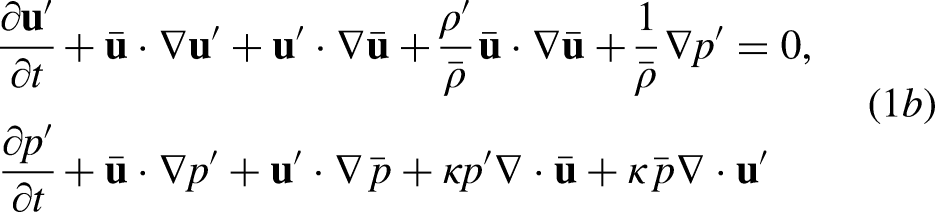
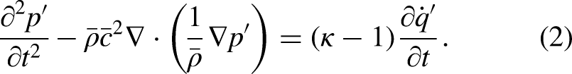
For a stagnant fluid, the linearized continuity equation is decoupled from the other equations. Subtracting the divergence of eq. (1b) multiplied by $\overline{\rho }{\overline{c}}^2$ from the time-derivative of eq. (1c) then leads to a wave equation for variable mean temperature fields similar to the one proposed by Cummings ¹⁴ :

$$\frac{{\mathrm{\partial }}^2{p}^{\mathrm{\prime }}}{\mathrm{\partial }{t}^2}-\overline{\rho }{\overline{c}}^2\mathrm{\nabla }\cdot \left(\frac{1}{\overline{\rho }}\mathrm{\nabla }{p}^{\mathrm{\prime }}\right)=(\kappa -1)\frac{\mathrm{\partial }{\dot{q}}^{\mathrm{\prime }}}{\mathrm{\partial }t}.$$

(2)In contrast to the explication of Cummings, this equation is not homentropic and does include entropy fluctuations in regions with non-vanishing mean flow entropy gradients. However, as such entropy fluctuations may only propagate via advection, they remain at their point of creation in this case of a stagnant fluid.

For a uniform mean flow velocity $\overline{\mathbf{u}}$ , Schuermans ²⁴ performs a coordinate transformation to a Lagrangian frame of reference moving with $\overline{\mathbf{u}}$ . As a result, the partial temporal derivative is transformed to a material derivative $\overline{\mathrm{D}}/\mathrm{D}t=\mathrm{\partial }/\mathrm{\partial }t+\overline{\mathbf{u}}\cdot \mathrm{\nabla }$ . Applying this method to eq. (2) leads to:

$${(\frac{\mathrm{\partial }}{\mathrm{\partial }t}+\overline{\mathbf{u}}\cdot \mathrm{\nabla })}^2{p}^{\mathrm{\prime }}-\overline{\rho }{\overline{c}}^2\mathrm{\nabla }\cdot \left(\frac{1}{\overline{\rho }}\mathrm{\nabla }{p}^{\mathrm{\prime }}\right)=0.$$

(3)Note that, combustion processes are normally subject to combined changes in the mean density and velocity and are thus precluded ( ${\dot{q}}^{\mathrm{\prime }}=0$ ) in eq. (3). As it is only valid for uniform mean flow fields, it is very limited in its applicability.

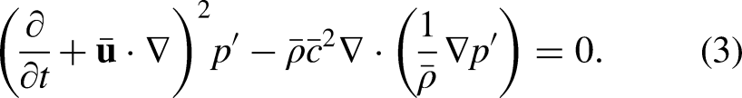
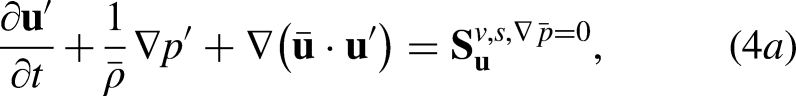
To obtain a universal formulation of eq. (3) for arbitrary mean flow fields including combustion, the LEE are transformed in a first step. As shown in Appendix A, the LEE inherently comprise acoustical, vortical and entropical modes. By filtering out the vortical and entropical components, the Acoustic Perturbation Equations (APE, (43)) result. As the APE represent pure acoustic wave propagation in arbitrary mean flow fields, they form an ideal base for the derivation of a universal convective wave equation as a second step. By exploiting the insignificant drop in mean pressure common to most technical combustion systems, the corresponding derivation is slightly simplified. From the mean momentum conservation equation, this gives $\mathrm{\nabla }\overline{p}/\overline{\rho }=\overline{\mathbf{u}}\cdot \mathrm{\nabla }\overline{\mathbf{u}}=0$ . Then, the closed set of the APE reads

$$\frac{\mathrm{\partial }{\mathbf{u}}^{\mathrm{\prime }}}{\mathrm{\partial }t}+\frac{1}{\overline{\rho }}\mathrm{\nabla }{p}^{\mathrm{\prime }}+\mathrm{\nabla }(\overline{\mathbf{u}}\cdot {\mathbf{u}}^{\mathrm{\prime }})={\mathbf{S}}_{\mathbf{u}}^{v,s,\mathrm{\nabla }\overline{p}=0},$$

(4a)

$$\frac{\mathrm{\partial }{p}^{\mathrm{\prime }}}{\mathrm{\partial }t}+\kappa \overline{p}\mathrm{\nabla }\cdot {\mathbf{u}}^{\mathrm{\prime }}+\overline{\mathbf{u}}\cdot \mathrm{\nabla }{p}^{\mathrm{\prime }}+\kappa p^{\mathrm{\prime }}\mathrm{\nabla }\cdot \overline{\mathbf{u}}=(\kappa -1){\dot{q}}^{\mathrm{\prime }},$$

(4b)with the momentum source ${\mathbf{S}}_{\mathbf{u}}^{v,s,\mathrm{\nabla }\overline{p}=0}$ exciting vortical and entropical modes. It is equivalent to eq. (44b) for uniform mean pressure fields. Following the procedure of Kotake ⁴ and Candel et al. ⁵ the divergence of eq. (4a) multiplied by $\overline{\rho }{\overline{c}}^2=\kappa \overline{p}$ is subtracted from the material derivative of eq. (4b). This leads to the acoustically consistent, inhomogeneous convective wave equation:

$$\begin{array}{rl}& \frac{{\mathrm{\partial }}^2{p}^{\mathrm{\prime }}}{\mathrm{\partial }{t}^2}+2\overline{\mathbf{u}}\cdot \mathrm{\nabla }\frac{\mathrm{\partial }{p}^{\mathrm{\prime }}}{\mathrm{\partial }t}+\overline{\mathbf{u}}\cdot \mathrm{\nabla }(\overline{\mathbf{u}}\cdot \mathrm{\nabla }{p}^{\mathrm{\prime }})-\overline{\rho }{\overline{c}}^2\mathrm{\nabla }\cdot \left(\frac{1}{\overline{\rho }}\mathrm{\nabla }{p}^{\mathrm{\prime }}\right)\\ & =-\kappa \frac{\mathrm{\partial }{p}^{\mathrm{\prime }}}{\mathrm{\partial }t}\mathrm{\nabla }\cdot \overline{\mathbf{u}}-\overline{\mathbf{u}}\cdot \mathrm{\nabla }(\kappa p^{\mathrm{\prime }}\mathrm{\nabla }\cdot \overline{\mathbf{u}})-\kappa \overline{p}(\overline{\mathbf{u}}\cdot \mathrm{\nabla })(\mathrm{\nabla }\cdot {\mathbf{u}}^{\mathrm{\prime }})\\ & +\kappa \overline{p}\mathrm{\Delta }(\overline{\mathbf{u}}\cdot {\mathbf{u}}^{\mathrm{\prime }})-\kappa \overline{p}\mathrm{\nabla }\cdot {\mathbf{S}}_{\mathbf{u}}^{v,s,\mathrm{\nabla }\overline{p}=0}\\ & +(\kappa -1)\frac{\mathrm{\partial }{\dot{q}}^{\mathrm{\prime }}}{\mathrm{\partial }t}+(\kappa -1)\overline{\mathbf{u}}\cdot \mathrm{\nabla }{\dot{q}}^{\mathrm{\prime }}.\end{array}$$

(5)Here, the left hand side (LHS) is reshaped into that of eq. (3), whereas the RHS contains all remaining terms. This equation is unclosed due to the terms depending on the velocity fluctuations on the RHS. These terms constitute sources and sinks for acoustic waves advected by the mean flow velocity $\overline{\mathbf{u}}$ .

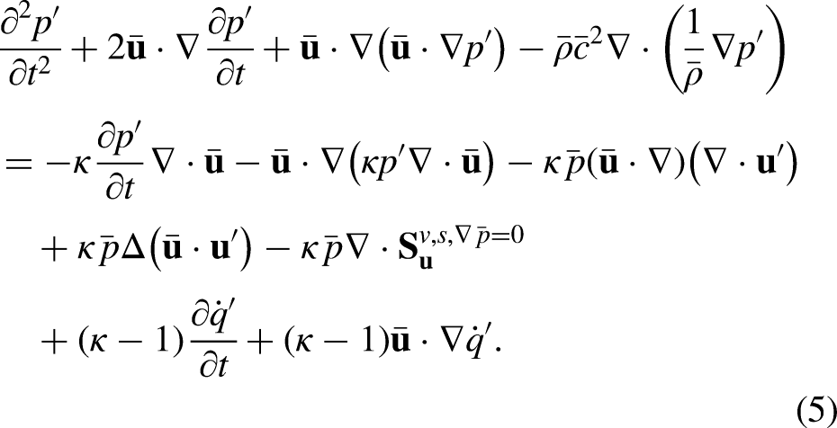
Linear acoustic fluctuations may be assumed to oscillate quasi-harmonically with exponentially growing or decaying amplitudes. The time-dependency may thus be expressed in the form ${\mathrm{\Phi }}^{\mathrm{\prime }}(t,\mathbf{x})=\hat{\mathrm{\Phi }}(\mathbf{x}){\mathrm{e}}^{\mathrm{i}\omega t}$ , where the complex angular frequency $\omega =2\pi f+\mathrm{i}\delta$ determines the oscillation frequency $f$ and the amplitude’s decay rate $\delta$ , which is just the negative growth rate $\delta =-\alpha$ . The hat denotes the complex valued spatial distribution of the arbitrary fluctuation quantity $\mathrm{\Phi }$ at the angular frequency $\omega$ . Inserting this approach into the above presented acoustically consistent, inhomogeneous convective wave equation (5) leads to the corresponding formulation in frequency domain:

$$\begin{array}{rl}& {\omega }^2\hat{p}-2\mathrm{i}\omega \overline{\mathbf{u}}\cdot \mathrm{\nabla }\hat{p}-\overline{\mathbf{u}}\cdot \mathrm{\nabla }(\overline{\mathbf{u}}\cdot \mathrm{\nabla }\hat{p})+\overline{\rho }{\overline{c}}^2\mathrm{\nabla }\cdot \left(\frac{1}{\overline{\rho }}\mathrm{\nabla }\hat{p}\right)\\ & =\mathrm{i}\omega \kappa \hat{p}\mathrm{\nabla }\cdot \overline{\mathbf{u}}+\overline{\mathbf{u}}\cdot \mathrm{\nabla }(\kappa \hat{p}\mathrm{\nabla }\cdot \overline{\mathbf{u}})+\kappa \overline{p}(\overline{\mathbf{u}}\cdot \mathrm{\nabla })(\mathrm{\nabla }\cdot \hat{\mathbf{u}})\\ & -\kappa \overline{p}\mathrm{\Delta }(\overline{\mathbf{u}}\cdot \hat{\mathbf{u}})+\kappa \overline{p}\mathrm{\nabla }\cdot {\hat{\mathbf{S}}}_{\mathbf{u}}^{v,s,\mathrm{\nabla }\overline{p}=0}\\ & -\mathrm{i}\omega (\kappa -1)\hat{\dot{q}}-(\kappa -1)\overline{\mathbf{u}}\cdot \mathrm{\nabla }\hat{\dot{q}}.\end{array}$$

(6)It is easy to prove that the entire RHS of eq. (5) and thus also of (6) vanishes for uniform mean flow fields. Then the convective wave equation according to eq. (3) is obtained. In frequency domain it reads

$${\omega }^2\hat{p}-2\mathrm{i}\omega \overline{\mathbf{u}}\cdot \mathrm{\nabla }\hat{p}-\overline{\mathbf{u}}(\overline{\mathbf{u}}\cdot \mathrm{\nabla })\cdot \mathrm{\nabla }\hat{p}+{\overline{c}}^2{\mathrm{\nabla }}^2\hat{p}=0.$$

(7)Recall that with the assumption of a uniform mean flow velocity in eq. (7) mean density gradients and thus also combustion processes are precluded. Equation (5) reduces to the inhomogeneous wave equation (2) for stagnant fluids with unsteady heat realease. Transformed to frequency domain, the inhomogeneous Helmholtz equation results:

$${\omega }^2\hat{p}+\overline{\rho }{\overline{c}}^2\mathrm{\nabla }\cdot \left(\frac{1}{\overline{\rho }}\mathrm{\nabla }\hat{p}\right)=-\mathrm{i}\omega (\kappa -1)\hat{\dot{q}}.$$

(8)With the zero Mach number assumption of eq. (8), the mean density is not subject to restrictions and a flame may be considered. Consequently, heat release fluctuations $\hat{\dot{q}}$ may be considered with eq. (8) but not with eq. (7). In order to attain an intelligible nomenclature, the convective wave equation in frequency domain will henceforth be referred to as convective Helmholtz equation despite being well aware that it does not satisfy the classic definition of the Helmholtz equation.

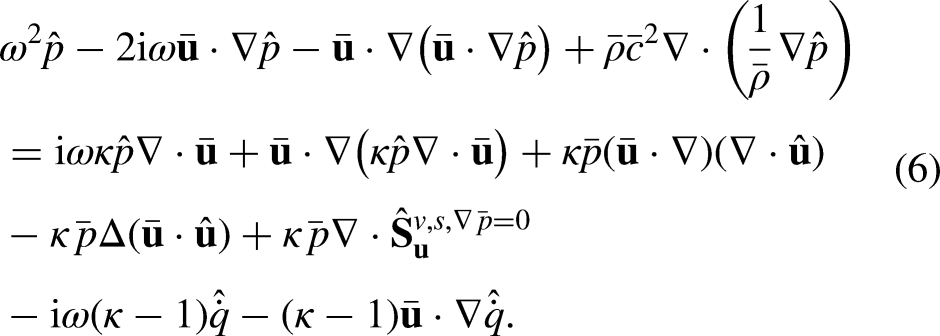
The Helmholtz equations (6)–(8) represent nonlinear eigenvalue problems. Their numerical solution using FEM methods will be discussed in the following section.

Weak Form of the Convective Helmholtz Equation

The Helmholtz equations discussed above are boundary value problems, whereas the corresponding wave equations additionally require initial values for the problem closure. Due to their frequency dependency, acoustic boundary conditions are quite straightforward to implement in the frequency domain. Therefore, the following derivation is exemplarily performed for the inhomogeneous convective Helmholtz equation (6). This also enables the pursued modal stability analysis, which is based on equations in the frequency domain. It may be noted that the derivations can be performed equivalently for the time-domain equations.

The basic idea of finite-element methods (FEM) is the satisfaction of the partial differential problem in a weak form within the entire computational domain in an integral sense. For further information on the spatial discretization in FEM, the reader is referred to Donea and Huerta ²⁵ . To obtain the weak form of eq. (6) for the use in FEM approaches, it is multiplied by the weighting function $\tilde{p}$ and integrated over the domain volume $V$ . Then, selected terms are integrated by parts. The detailed procedure is demonstrated in Appendix B, which ultimately yields the weak form of the inhomogeneous convective Helmholtz equation (iCHE)

$$\begin{array}{rl}& \int \int {\int }_V\{{\omega }^2\hat{p}\tilde{p}-\mathrm{i}\omega (\overline{\mathbf{u}}\cdot \mathrm{\nabla }\hat{p})\tilde{p}+\mathrm{i}\omega \hat{p}\overline{\mathbf{u}}\cdot \mathrm{\nabla }\tilde{p}\\ & +(\overline{\mathbf{u}}\cdot \mathrm{\nabla }\hat{p})\overline{\mathbf{u}}\cdot \mathrm{\nabla }\tilde{p}-{\overline{c}}^2\mathrm{\nabla }\hat{p}\cdot \mathrm{\nabla }\tilde{p}\}\mathrm{d}V\\ & -\int {\int }_{\mathrm{\Omega }}\mathbf{F}\cdot \mathbf{n}\tilde{p}\mathrm{d}\mathrm{\Omega }=\int \int {\int }_V{S}_{iCHE}\tilde{p}\mathrm{d}V.\end{array}$$

(9)The LHS of this equation equals the weak formulation of the homogeneous convective wave equation in frequency domain for uniform mean flow velocities. This also applies to the flux $\mathbf{F}$ across the boundary $\mathrm{\Omega }$ , which reads

$$\mathbf{F}=\mathrm{i}\omega \overline{\mathbf{u}}\hat{p}+\overline{\mathbf{u}}(\overline{\mathbf{u}}\cdot \mathrm{\nabla }\hat{p})-{\overline{c}}^2\mathrm{\nabla }\hat{p}.$$

(10)Interactions of the advected waves with mean flow gradients are described by the RHS volume sources $S_{iCHE}$ :

$$\begin{array}{cc}{S}_{iCHE}& =\mathrm{i}\omega (\kappa -1)\hat{p}\mathrm{\nabla }\cdot \overline{\mathbf{u}}+\kappa \hat{p}\overline{\mathbf{u}}\cdot \mathrm{\nabla }(\mathrm{\nabla }\cdot \overline{\mathbf{u}})\\ & +(\kappa -1)(\overline{\mathbf{u}}\cdot \mathrm{\nabla }\hat{p})(\mathrm{\nabla }\cdot \overline{\mathbf{u}})-\kappa \overline{p}\mathrm{\Delta }(\overline{\mathbf{u}}\cdot \hat{\mathbf{u}})\\ & +\kappa \overline{p}\mathrm{\nabla }\cdot {\hat{\mathbf{S}}}_{\mathbf{u}}^{v,s,\mathrm{\nabla }\overline{p}=0}+\kappa \overline{p}(\overline{\mathbf{u}}\cdot \mathrm{\nabla })(\mathrm{\nabla }\cdot \hat{\mathbf{u}})\\ & \mathrm{i}\omega (\kappa -1)\hat{\dot{q}}-(\kappa -1)\overline{\mathbf{u}}\cdot \mathrm{\nabla }\hat{\dot{q}},\end{array}$$

(11)They are a measure of the errors introduced when applying the homogeneous convective wave equation to arbitrary mean flow fields.

In order to transform the boundary flux into a universal Neumann boundary condition, a basic set of equations complying with the assumption of a uniform mean flow velocity is required. This set is provided by the afore presented APE (4a) and (4b). In frequency domain, they read for a uniform mean flow velocity with vanishing heat release

$$\mathrm{i}\omega \hat{\mathbf{u}}+\frac{1}{\overline{\rho }}\mathrm{\nabla }\hat{p}+\overline{\mathbf{u}}\cdot \mathrm{\nabla }\hat{\mathbf{u}}=0,$$

(12a)

$$\mathrm{i}\omega \hat{p}+\kappa \overline{p}\mathrm{\nabla }\cdot \hat{\mathbf{u}}+\overline{\mathbf{u}}\cdot \mathrm{\nabla }\hat{p}=0.$$

(12b)Combining this linearized momentum and energy equation according to $\overline{\mathbf{u}}$ (12b) $-\overline{\rho }{\overline{c}}^2$ (12a) and exploiting the vector identity $\mathrm{\nabla }\times (\hat{\mathbf{u}}\times \overline{\mathbf{u}})=\overline{\mathbf{u}}\cdot \mathrm{\nabla }\hat{\mathbf{u}}-\overline{\mathbf{u}}(\mathrm{\nabla }\cdot \hat{\mathbf{u}})+\hat{\mathbf{u}}(\mathrm{\nabla }\cdot \overline{\mathbf{u}})-\hat{\mathbf{u}}\cdot \mathrm{\nabla }\overline{\mathbf{u}}$ , the boundary flux $\mathbf{F}$ can be transformed into

$$\begin{array}{cc}\mathbf{F}& =\mathrm{i}\omega \overline{\rho }{\overline{c}}^2\hat{\mathbf{u}}+\kappa \overline{p}(\overline{\mathbf{u}}\cdot \mathrm{\nabla }\hat{\mathbf{u}}-\overline{\mathbf{u}}(\mathrm{\nabla }\cdot \hat{\mathbf{u}}))\\ & =\mathrm{i}\omega \overline{\rho }{\overline{c}}^2\hat{\mathbf{u}}+\kappa \overline{p}\mathrm{\nabla }\times (\hat{\mathbf{u}}\times \overline{\mathbf{u}}).\end{array}$$

(13)When introducing the above stated vector identity, consistent use was made of the uniform mean flow velocity presumed for the entire LHS of eq. (49). The newly emerging term containing the rotation of the mean flow and perturbation velocity’s vector product requires further explication. That term vanishes only if the velocity vectors of perturbation and mean flow are pointing in the same direction. This applies particularly for flow regimes which may be characterized as one-dimensional. In many practical applications, the assumption of one-dimensionality is an essential feature. It is for instance used in the well-established Multi-Microphone Method to measure acoustic characteristics of components. The same purpose is served by low-order network models, which provide acoustic characterizations of components based on analytic expressions. Such network models for one-dimensional acoustic propagation are discussed in more detail below. Both approaches are only valid, if the hydraulic diameter $d_h$ of the investigated component is acoustically compact. This condition forms the basis for one-dimensional wave propagation and may be expressed in terms of the Helmholtz number as $\mathrm{He}=k{d}_h\ll 1$ with the wave number $k$ .

Normally, an overall system boundary consists of different types of sub boundaries, which can be classified by their acoustic scattering characteristics. Common types include boundaries open to the atmosphere and rigid wall boundaries. While the former boundary type exhibits a constant pressure, the latter type is characterized by a vanishing surface normal velocity ( $\overline{\mathbf{u}}\cdot \mathbf{n}=\hat{\mathbf{u}}\cdot \mathbf{n}=0$ , with $\mathbf{n}$ denoting the outward pointing surface normal vector). As a consequence, the weak form flux of eq. (13) also vanishes at wall boundaries. If the remaining sub boundaries ${\mathrm{\Omega }}_j$ of the overall system boundary are acoustically compact, one-dimensional approaches may be applied as discussed above. Then the boundary flux simplifies to

$$\mathbf{F}=\mathrm{i}\omega \overline{\rho }{\overline{c}}^2\hat{\mathbf{u}},$$

(14)which solely depends on the velocity fluctuations. In a pure acoustic sense, this result directly corresponds to the aspired natural Neumann boundary condition.

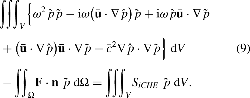
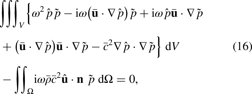
To conclude this section, the iCHE being the weak formulation of the acoustically consistent inhomogeneous Helmholtz equation (6), finally yields

$$\begin{array}{rl}& \int \int {\int }_V\{{\omega }^2\hat{p}\tilde{p}-\mathrm{i}\omega (\overline{\mathbf{u}}\cdot \mathrm{\nabla }\hat{p})\tilde{p}+\mathrm{i}\omega \hat{p}\overline{\mathbf{u}}\cdot \mathrm{\nabla }\tilde{p}\\ & +(\overline{\mathbf{u}}\cdot \mathrm{\nabla }\hat{p})\overline{\mathbf{u}}\cdot \mathrm{\nabla }\tilde{p}-{\overline{c}}^2\mathrm{\nabla }\hat{p}\cdot \mathrm{\nabla }\tilde{p}\}\mathrm{d}V\\ & -\int {\int }_{\mathrm{\Omega }}\mathrm{i}\omega \overline{\rho }{\overline{c}}^2\hat{\mathbf{u}}\cdot \mathbf{n}\tilde{p}\mathrm{d}\mathrm{\Omega }=\int \int {\int }_V{S}_{iCHE}\tilde{p}\mathrm{d}V.\end{array}$$

(15)With the assumptions of a uniform mean flow without heat release, the entire RHS of the former equation vanishes, leading to the weak formulation of the homogeneous convective Helmholtz equation (hCHE):

$$\begin{array}{rl}& \int \int {\int }_V\{{\omega }^2\hat{p}\tilde{p}-\mathrm{i}\omega (\overline{\mathbf{u}}\cdot \mathrm{\nabla }\hat{p})\tilde{p}+\mathrm{i}\omega \hat{p}\overline{\mathbf{u}}\cdot \mathrm{\nabla }\tilde{p}\\ & +(\overline{\mathbf{u}}\cdot \mathrm{\nabla }\hat{p})\overline{\mathbf{u}}\cdot \mathrm{\nabla }\tilde{p}-{\overline{c}}^2\mathrm{\nabla }\hat{p}\cdot \mathrm{\nabla }\tilde{p}\}\mathrm{d}V\\ & -\int {\int }_{\mathrm{\Omega }}\mathrm{i}\omega \overline{\rho }{\overline{c}}^2\hat{\mathbf{u}}\cdot \mathbf{n}\tilde{p}\mathrm{d}\mathrm{\Omega }=0,\end{array}$$

(16)which is the weak form counterpart of eq. (7). For stagnant fluids, the iCHE (15) simplifies to the weak formulation of the Helmholtz equation (8) (denoted with HE):

$$\begin{array}{rl}& \int \int {\int }_V\{{\omega }^2\hat{p}\tilde{p}-{\overline{c}}^2\mathrm{\nabla }\hat{p}\cdot \mathrm{\nabla }\tilde{p}\}\mathrm{d}V\\ & +\int {\int }_{\mathrm{\Omega }}\mathrm{i}\omega \overline{\rho }{\overline{c}}^2\hat{\mathbf{u}}\cdot \mathbf{n}\tilde{p}\mathrm{d}\mathrm{\Omega }=-\int \int {\int }_V\mathrm{i}\omega (\kappa -1)\hat{\dot{q}}\tilde{p}\mathrm{d}V.\end{array}$$

(17)Note that the second term within the volume integral on the LHS of eq. (17) is equally valid for mean flow fields with and without mean density gradients. Therefore, this weak form corresponds to the Sturm-Liouville Problem in frequency domain, which was initially proposed by Cummings ¹⁴ for acoustic wave propagation in media with temperature gradients.

Acoustic Boundary Conditions

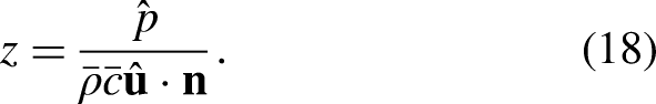
The boundary flux of the weak formulations discussed in the previous section can be further generalized for the application of frequency dependent acoustic boundary conditions. A commonly applied boundary condition is the specific impedance, which is defined as

$$z=\frac{\hat{p}}{\overline{\rho }\overline{c}\hat{\mathbf{u}}\cdot \mathbf{n}}.$$

(18)The boundary flux thus becomes a function of the state variable $\hat{p}$ and the specific impedance

$$\mathrm{F}=\mathrm{i}\omega \overline{\rho }{\overline{c}}^2\hat{\mathbf{u}}\cdot \mathbf{n}=\mathrm{i}\omega \overline{c}\frac{\hat{p}}{z},$$

(19)which represents a boundary condition of the third kind. The same result is obtained for the weak formulations of the homogeneous convective Helmholtz equation (16) and the Helmholtz equation (17) when using the corresponding formulations of linearized momentum and energy equations to transform the remaining flux terms.

The impedance boundary condition as defined in eq. (18) poses an acoustic one-port terminating a domain. For the coupling of two spatially disconnected domains, acoustic two-ports can be employed. Such an acoustic two-port is the transfer matrix, which couples the acoustic fluctuations at the downstream domain (index $d$ ) with those at the upstream domain (index $u$ ). In terms of the primitive variables $\hat{p}$ and $\hat{\mathbf{u}}$ , the transfer matrix coupling yields

$$\begin{array}{cc}{\left(\begin{array}{c}\frac{\hat{p}}{\overline{\rho }\overline{c}}\\ -\hat{\mathbf{u}}\cdot \mathbf{n}\end{array}\right)}_d& =\mathbf{T}\mathbf{M}{\left(\begin{array}{c}\frac{\hat{p}}{\overline{\rho }\overline{c}}\\ \hat{\mathbf{u}}\cdot \mathbf{n}\end{array}\right)}_u\\ & =\left(\begin{array}{cc}{\mathrm{TM}}_{11}& {\mathrm{TM}}_{12}\\ {\mathrm{TM}}_{21}& {\mathrm{TM}}_{22}\end{array}\right){\left(\begin{array}{c}\frac{\hat{p}}{\overline{\rho }\overline{c}}\\ \hat{\mathbf{u}}\cdot \mathbf{n}\end{array}\right)}_u.\end{array}$$

(20)The concepts of one- and two-ports stems from one-dimensional acoustic theory. To account for the discrepancy of the one-dimensional formulation of the transfer matrix and its application to boundaries with arbitrary spatial orientation, only the boundary normal velocity component must be used. The negative sign at the downstream side results from the opposite orientation of the normal vectors at the two sides. At the downstream side, this normal vector points in the opposite direction of positive one-dimensional velocity fluctuations.

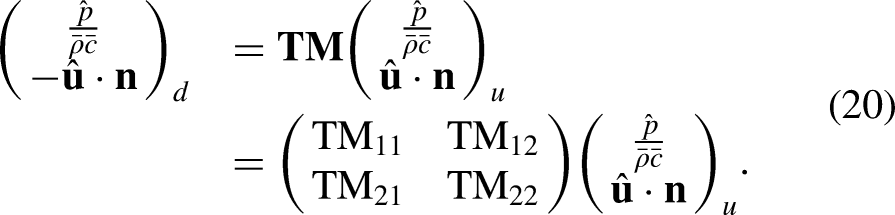
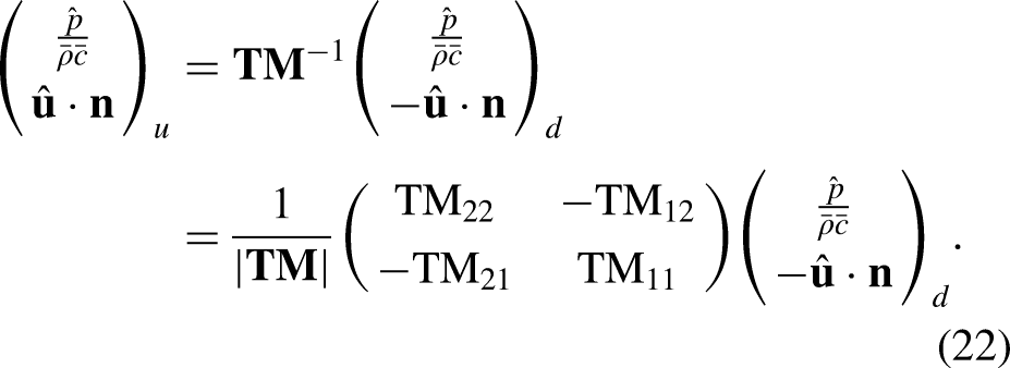
An ordinary way to determine acoustic transfer matrices of components is the use of one-dimensional low-order network models. These are normally derived from equations subject to restrictive assumptions like homentropic and irrotational flows. To consistently integrate the network models into the numeric model of the Helmholtz equations requires a consistent implementation of restrictions at the boundaries. The weak form flux of eq. (10) is based on the convective Helmholtz equation for uniform mean flows without heat release. Therefore, the consistency in terms of homentropicity and irrotationality is given for this boundary flux formulation. Furthermore, the one-dimensionality of transfer matrices coincides with the assumption of acoustically compact sub-boundaries exploited for eq. (14). Recall that the weak form flux of the Helmholtz equations is then directly proportional to the acoustic velocity fluctuations. In this case the native formulation of the transfer matrix is very useful for the implementation of a coupling boundary condition. In particular the second equation provides the acoustic velocity at the downstream boundary as a function of the primitive variables at the upstream boundary. By using eq. (14) the velocity fluctuation at the upstream side can be expressed as an exclusive function of the solution variable $\hat{p}$ . The weak form flux at the downstream coupling boundary ${\mathbf{F}}_d$ then yields

$$\begin{array}{rl}{\mathrm{F}}_d& =\int {\int }_{{\mathrm{\Omega }}_u}\{\mathrm{i}\omega \overline{c}{\mathrm{TM}}_{21}\hat{p}\\ & +{\mathrm{TM}}_{22}(\mathrm{i}\omega \overline{\mathbf{u}}\hat{p}+\overline{\mathbf{u}}(\overline{\mathbf{u}}\cdot \mathrm{\nabla }\hat{p})-{\overline{c}}^2\mathrm{\nabla }\hat{p})\cdot \mathbf{n}\}\tilde{p}\mathrm{d}{\mathrm{\Omega }}_u.\end{array}$$

(21)To obtain an equivalent formulation for the upstream boundary, the transfer matrix definition (20) is inverted first:

$$\begin{array}{rl}{\left(\begin{array}{c}\frac{\hat{p}}{\overline{\rho }\overline{c}}\\ \hat{\mathbf{u}}\cdot \mathbf{n}\end{array}\right)}_u& ={\mathbf{T}\mathbf{M}}^{-1}{\left(\begin{array}{c}\frac{\hat{p}}{\overline{\rho }\overline{c}}\\ -\hat{\mathbf{u}}\cdot \mathbf{n}\end{array}\right)}_d\\ & =\frac{1}{\left|\mathbf{T}\mathbf{M}\right|}\left(\begin{array}{cc}{\mathrm{TM}}_{22}& -{\mathrm{TM}}_{12}\\ -{\mathrm{TM}}_{21}& {\mathrm{TM}}_{11}\end{array}\right){\left(\begin{array}{c}\frac{\hat{p}}{\overline{\rho }\overline{c}}\\ -\hat{\mathbf{u}}\cdot \mathbf{n}\end{array}\right)}_d.\end{array}$$

(22)Again, the second equation gives direct access to the sought after velocity fluctuation at the upstream coupling boundary. The corresponding weak form flux reads

$$\begin{array}{rl}{\mathrm{F}}_u& =\frac{1}{\left|\mathbf{T}\mathbf{M}\right|}\int {\int }_{{\mathrm{\Omega }}_d}\{\mathrm{i}\omega \overline{c}{\mathrm{TM}}_{21}\hat{p}\\ & +{\mathrm{TM}}_{11}(\mathrm{i}\omega \overline{\mathbf{u}}\hat{p}+\overline{\mathbf{u}}(\overline{\mathbf{u}}\cdot \mathrm{\nabla }\hat{p})-{\overline{c}}^2\mathrm{\nabla }\hat{p})\\ & \cdot \mathbf{n}\}\tilde{p}\mathrm{d}{\mathrm{\Omega }}_d,\end{array}$$

(23)which is an exclusive function of the solution variable at the downstream coupling boundary.

Industrial Gas Turbine Combustor Model

To investigate the applicability of the different Helmholtz equations’ weak formulations (15)–(17) to arbitrary mean flow fields, an industrial combustion system is modeled. The targeted system is a can annular combustion chamber of a Siemens H-class gas turbine as schematically shown in Fig. 1.

Figure 1.

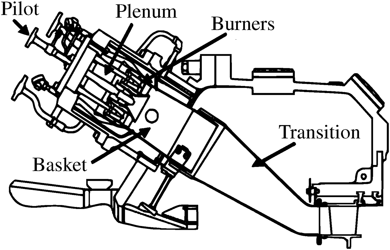
Typical Siemens can annular combustion chamber adopted from Sattelmayer et al. ²⁶ .

The modeling strategy of this setup is similar to the one discussed by Campa and Camporeale ²⁷ : The plenum and the actual combustion chamber consisting of the basket and the transition are resolved by means of FEM. The slightly simplified and disconnected three-dimensional computational domain of the combustor including the tetrahedral mesh with approximately 280k elements is presented in Fig. 2. As the geometrical resolution of the interconnecting burners including the swirlers would highly increase the computational cost, they are replaced by a transfer matrix obtained from a one-dimensional network model. Instead of the geometrically resolved burners, the corresponding burner transfer matrix then couples the two disconnected domains via the respective coupling boundaries, highlighted in blue in the bottom images of Fig. 2.

Figure 2.

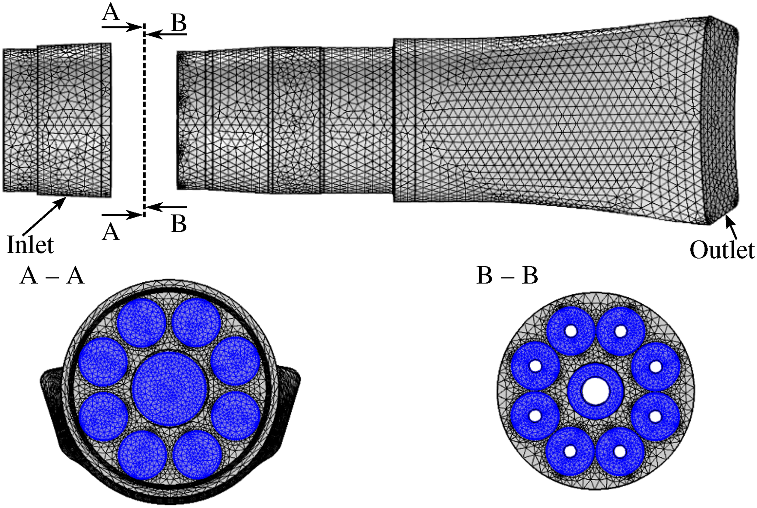
Top: Split computational domains including the corresponding unstructured tetrahedral mesh of the investigated H-class combustor. Bottom left: View on the basket’s face plate with the downstream coupling surfaces of the burners highlighted in blue. Bottom right: View on the plenum’s face plate with the upstream coupling surfaces of the burners highlighted in blue.

The wall boundaries and the circumferential mean flow inlet boundary at the plenum are specified to have zero fluctuating mass flow. This corresponds to a specific impedance of

$$z_{\hat{\dot{m}}=0}=-\frac{\overline{c}}{\overline{\mathbf{u}}\cdot \mathbf{n}}.$$

(24)The turbine inlet downstream of the transition represents the combustion chamber’s outlet. For this boundary, zero total enthalpy fluctuations are imposed, which can be expressed as

$$z_{{\hat{h}}_0=0}=-\frac{\overline{\mathbf{u}}\cdot \mathbf{n}}{\overline{c}}$$

(25)in terms of a specific impedance. Both types of boundary conditions are energetically neutral. This means that no acoustic energy enters or leaves the domains across the corresponding boundaries, even in the presence of a mean mass flux. For the Helmholtz equation a stagnant fluid is presumed, which also results in zero mean mass fluxes at the boundaries. In this case, $z_{\hat{\dot{m}}=0}$ corresponds to an acoustic wall (i.e. sound hard) boundary, whereas $z_{{\hat{h}}_0=0}$ represents an open end (i.e. sound soft) boundary.

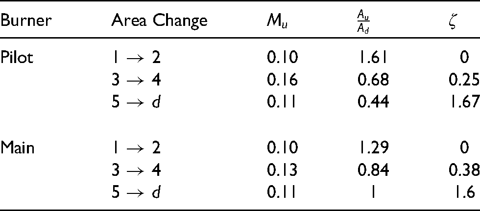
The two domains of plenum and combustion chamber are linked via a central pilot and eight circumferentially distributed main burners. Each of the burners is replaced by a transfer matrix to couple an upstream coupling surface of the plenum with the corresponding downstream counterpart of the combustion chamber. The transfer matrix is obtained from a simple low-order network model, which had been discussed e.g. by Sattelmayer and Polifke ²⁸ for thermoacoustic systems. The schematic in Fig. 3 represents the network used to describe the acoustic transfer behavior of the burners. It consists of simple acoustic elements, in particular duct elements and sudden area changes.

Figure 3.

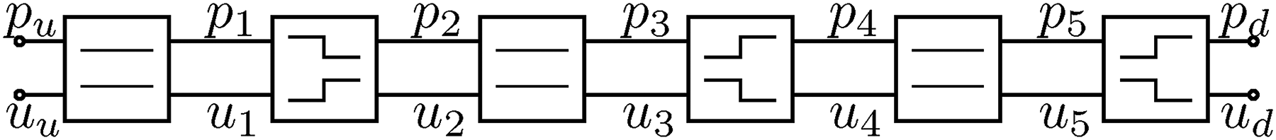
Low-order network model to describe the acoustic transfer behavior of the burners.

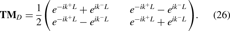
Ducts can be interpreted as time lag elements for traveling waves. In terms of a transfer matrix their transfer behavior can be described as ²⁹

$${\mathbf{T}\mathbf{M}}_D=\frac{1}{2}(\begin{array}{cc}{e}^{-i{k}^{+}L}+e^{i{k}^{-}L}& e^{-i{k}^{+}L}-e^{i{k}^{-}L}\\ e^{-i{k}^{+}L}-e^{i{k}^{-}L}& e^{-i{k}^{+}L}+e^{i{k}^{-}L}\end{array}).$$

(26)Here, $L$ is the length of the duct and $k^{\pm }=\omega /(\overline{c}\pm \overline{u})$ is the wave number subject to a mean flow velocity. The interactions of acoustic waves and the separated mean flow at a sudden area change normally constitute complex fluid dynamic processes. These interactions cause an energy transfer between acoustical and vortical fluctuations, which had been filtered from the LEE to derive the APE. This effect can be accounted for by introducing a static pressure loss to the linearized Bernoulli equation for homentropic and irrotational flows. In combination with a linearized continuity equation, Gentemann et al. ³⁰ and Schuermans ²⁴ then derive a transfer matrix of the compact element. For the present work, capacitance and inertial effects are neglected, which leads to the simplified formulation

$${\mathbf{T}\mathbf{M}}_{AC}=\left(\begin{array}{cc}1& -M_u({\left(\frac{A_u}{A_d}\right)}^2+\zeta -1)\\ 0& \frac{A_u}{A_d}\end{array}\right).$$

(27)The pressure loss coefficient

$$\zeta =\frac{\mathrm{\Delta }{p}_L}{\frac{\overline{\rho }}{2}{\overline{u}}_u^2}$$

(28)relates the static pressure loss across the area change to the dynamic pressure head at the upstream side of the element. At this location also the local Mach number $M_u$ is evaluated. Basically, the network of the burners as depicted in Fig. 3 consists of three duct elements connected by sudden area changes. The central duct element exhibits a smaller cross-sectional area than the remaining ducts. This mimics the constriction of the streamlines due to the burner’s swirler vanes. The trailing area change is mainly included to impinge acoustic losses that are expected to be induced at the interface of burners and face plate due to flow separation. Multiplying the transfer matrices of the single network elements according to

$${\mathbf{T}\mathbf{M}}_{burner}={\mathbf{T}\mathbf{M}}_N\cdot {\mathbf{T}\mathbf{M}}_{N-1}\cdot \dots \cdot {\mathbf{T}\mathbf{M}}_1$$

(29)finally yields the complete burner transfer matrix. The indices represent the location of the element in the network from upstream to downstream in ascending order. The parameters of the sudden area changes for the pilot and the main burners are listed in Tab. 1. The specified pressure loss coefficients correspond to a static pressure loss of 2% across the burners.

Table 1.

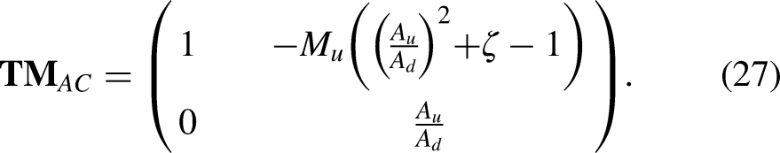
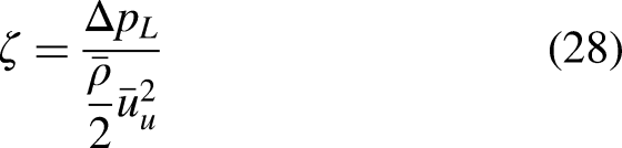
Parameters of the three area changes within the low-order network to acoustically describe the pilot and the main burners. The naming is in accordance with Fig. 3.

Burner	Area Change	$M_u$	$\frac{A_u}{A_d}$	$\zeta$
Pilot	1 $\to$ 2	0.10	1.61	0
	3 $\to$ 4	0.16	0.68	0.25
	5 $\to$ $d$	0.11	0.44	1.67
Main	1 $\to$ 2	0.10	1.29	0
	3 $\to$ 4	0.13	0.84	0.38
	5 $\to$ $d$	0.11	1	1.6

The parameters of the network model are in accordance with the mean field data used for the acoustic computations. This data was provided by Siemens Energy for an operation point at part load. It stems from a reactive Unsteady Reynolds-Averaged Navier-Stokes (URANS) simulation using a Burning Velocity Model (BVM). For turbulent closure of the governing equations, a modified SST model was applied. Note that the numerical setup of the CFD simulations and the corresponding results have not been published by Siemens Energy. Figure 4 shows a cross-section of the computational domain with the interpolated mean temperature field obtained from the time-averaged URANS results.

Figure 4.

Mean temperature field interpolated on the FEM mesh of the H-class combustion chamber. The cross-sectional view also highlights the excluded burner geometries. The field data was provided by Siemens Energy.

Investigated Numerical Setups

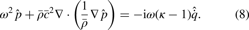
The different Helmholtz equations are applied in a comparative modal stability analysis of the H-class combustor model presented in the previous section. The investigated numerical setups are specified in Tab. 2. As a reference setup, the APE (4) are solved in frequency domain (FD). They are simplified by assuming a passive flame, i.e. 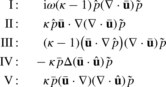$\widehat{.q}=0$ . Furthermore, specifying ${\mathbf{S}}_{\mathbf{u}}^{v,s,\mathrm{\nabla }\overline{p}=0}=0$ prevents any interaction mechanisms between acoustic and vortical modes. Therefore, this set of equations is considered to consistently describe acoustic wave propagation in arbitrary mean flow fields. With these simplifications, the RHS source of the iCHE (11) reduces to five terms, which are assigned with roman numbers:

$$\begin{array}{rl}\mathrm{I}:& \phantom{-}\mathrm{i}\omega (\kappa -1)\hat{p}(\mathrm{\nabla }\cdot \overline{\mathbf{u}})\tilde{p}\\ \mathrm{II}:& \phantom{-}\kappa \hat{p}\overline{\mathbf{u}}\cdot \mathrm{\nabla }(\mathrm{\nabla }\cdot \overline{\mathbf{u}})\tilde{p}\\ \mathrm{III}:& \phantom{-}(\kappa -1)(\overline{\mathbf{u}}\cdot \mathrm{\nabla }\hat{p})(\mathrm{\nabla }\cdot \overline{\mathbf{u}})\tilde{p}\\ \mathrm{IV}:& -\kappa \overline{p}\mathrm{\Delta }(\overline{\mathbf{u}}\cdot \hat{\mathbf{u}})\tilde{p}\\ \mathrm{V}:& \phantom{-}\kappa \overline{p}(\overline{\mathbf{u}}\cdot \mathrm{\nabla })(\mathrm{\nabla }\cdot \hat{\mathbf{u}})\tilde{p}\end{array}$$

Due to the source terms depending on the velocity fluctuations (IV and V) the acoustically consistent iCHE (15) is still unclosed, which prevents a straightforward implementation to FEM tools. Instead, the iCHE setup is only investigated with the first three source terms (I - III) and their impact on the stability analysis. The significance of the remaining source terms IV and V on the stability predictions with the iCHE can then be deduced from deviations from the APE, which are physically equivalent to the iCHE including all five source terms (I - V). Entirely neglecting the RHS source terms yields the hCHE according to eq. (16). By specifying a stagnant mean velocity field, the HE (17) automatically results from the iCHE.

Table 2.

Overview of the investigated numerical setups.

Setup ID	Eq.	Mean Flow	RHS Sources	BC
APE	4 (FD)	${\overline{\mathbf{u}}}_{CFD}$	0	$z$ / ${\mathbf{T}\mathbf{M}}_{burner}$
iCHE	15	${\overline{\mathbf{u}}}_{CFD}$	I-III	$z$ / ${\mathbf{T}\mathbf{M}}_{burner}$
hCHE-1	16	${\overline{\mathbf{u}}}_{CFD}$	0	$z$ / ${\mathbf{T}\mathbf{M}}_{burner}$
hCHE-2	16	${\overline{\mathbf{u}}}_{CFD}$	0	$z^{M=0}$ / ${\mathbf{T}\mathbf{M}}_{burner}^{M=0}$
HE	17	0	0	$z^{M=0}$ / ${\mathbf{T}\mathbf{M}}_{burner}^{M=0}$
eiHE	17	0	0	$z$ / ${\mathbf{T}\mathbf{M}}_{burner}$

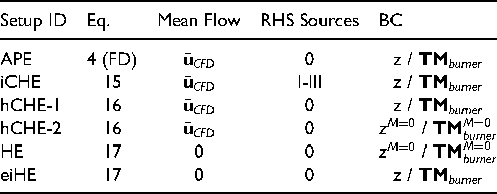
The boundary conditions and the burner transfer matrix (BTM) applied for the APE and the iCHE comply with the mean velocity field from CFD as described in the previous section. When applying the same boundary conditions to the HE with its zero Mach number assumption, energetic errors are introduced due to the dropped advection of acoustic energy. To still preserve comparability of the equations in terms of an energetic consistency, the impedance boundary conditions and the transfer matrices need to be energetically transformed. This procedure including the mathematical background is discussed in detail by Heilmann et al. ³¹ and leads to the energetically consistent boundary conditions $z^{M=0}$ and ${\mathbf{T}\mathbf{M}}_{burner}^{M=0}$ . As the hCHE also incorporates the advection of acoustic waves, the energetically consistent formulation must be applied with the original boundary conditions $z$ and ${\mathbf{T}\mathbf{M}}_{burner}$ . This setup (hCHE-1) is expected to exhibit deviations to the reference APE system due to the neglected interaction mechanisms between acoustics and mean flow non-uniformity. Additionally dropping the energetic consistency by using the boundary conditions for zero Mach number domains ( $z^{M=0}$ and ${\mathbf{T}\mathbf{M}}_{burner}^{M=0}$ ) is then expected to introduce further errors for the setup hCHE-2. However, this approach was applied by Kim et al. ²³ to investigate the stability of rocket engines, which delivered satisfying results. Finally, the energetic errors expected with the hCHE setups are compared to those of an energetically inconsistent Helmholtz equation (eiHE). For this Helmholtz setup the boundary conditions of the reference APE system are employed, which yields inconsistent energetic fluxes at the boundaries.

While the impedances $z_{\hat{\dot{m}}=0}$ and $z_{{\hat{h}}_0=0}$ are energetically neutral, the BTM ( ${\mathbf{T}\mathbf{M}}_{burner}$ ) incorporates acoustic dissipation due to the static pressure loss. In combination with the passive flame ( $\hat{\dot{q}}=0$ ) and the neglected acoustic-vortical interaction mechanisms ( ${\mathbf{S}}_{\mathbf{u}}^{v,s,\mathrm{\nabla }\overline{p}=0}=0$ ), the dissipation within the burners is the only physical mechanism contributing to the energy balance of the reference system APE.

The weak form of the equations for the setups listed in Tab. 2 and their corresponding boundary conditions are implemented in COMSOL Multiphysics using the Weak Form PDE-Module. The nonlinear eigenvalue problems constituted by the Helmholtz setups are linearized using a state-space representation as described by Schuermans ²⁴ . This procedure results in a duplication of state variables. Using the frequency dependent transfer matrix coefficients still yields a nonlinearity. It can be linearized as proposed by Jaensch et al. ³² : By deploying a transfer function fitting procedure to the frequency dependent coefficients, the resulting transfer function can be transformed into a linear state-space representation. For the solution of the linearized eigenvalue problems, the standard Eigenvalue-Solver with the default settings of COMSOL Multiphysics was used.

Despite the duplication of state-variables due to the linearization of the Helmholtz setups, the APE constituting a system of four equations are still computationally more demanding. Therefore, only a linear element order was viable for the mesh of Lagrangian elements presented in the preceding section. For the Helmholtz equations on the other hand, a quadratic element order was feasible and lead to robust, mesh independent results.

Comparative Modal Stability Analysis

The modal stability analyses of the H-class combustor model are performed in the low to intermediate frequency regime. This is in accordance with the requirement of acoustically compact boundary conditions when using the boundary flux expression (14). In the stability map of Fig. 5 firstly the eigenvalues of the APE are compared to those of the HE and the energetically consistent hCHE-1. The damping rate is plotted over the Helmholtz number $\mathrm{He}=2\pi f/({\overline{c}}_c{d}_{CC})$ , which relates the oscillation frequency to the cold flow speed of sound ${\overline{c}}_c$ and the diameter of the combustion chamber’s face plate $d_{CC}$ .

Figure 5.

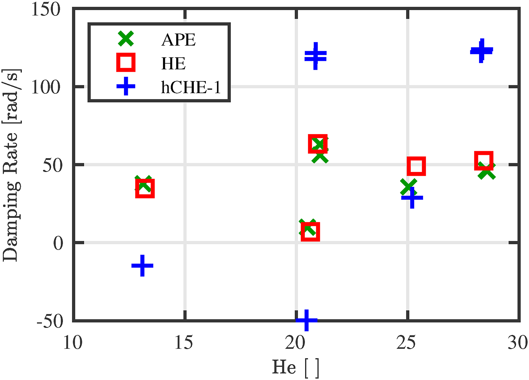
Stability map comparing the complex eigenfrequencies of the APE with those of the Helmholtz equation (HE) and the energetically consistent homogeneous convective Helmholtz equation (hCHE-1).

The pure acoustic mode shapes obtained from the HE setup corresponding to the eigenvalues are exhibited in Fig. 6. The first, second and fourth eigenmodes are longitudinal (Fig. 6 a), b) and d)), whereas the third and fifth modes are of transversal type, mainly oscillating in the plenum (Fig. 6 c) and e)). The latter types appear as mode pairs with a spatial phase shift of $\pi /2$ . Due to the lack of mean flow and a nearly symmetrical mean temperature field in the plenum, the individual eigenfrequencies of the pairs can not be distinguished in Fig. 5 for the HE setup.

Figure 6.

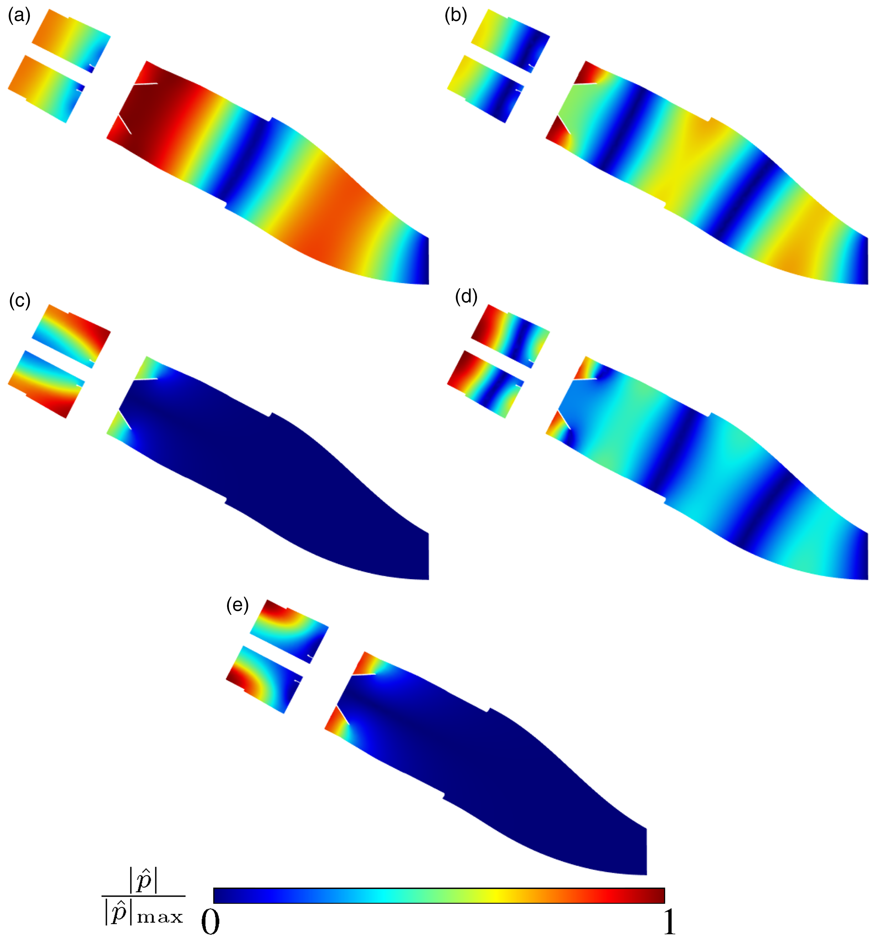
Acoustic mode shapes of the Helmholtz equation (HE; red squares $\mathbf{\text{□}}$ in Fig. 5) with ascending oscillation frequencies. Only one eigenmode is plotted for the degenerate transversal mode pairs c) and e). The eigenmodes a), b) and d) are longitudinal modes.

As expected, the reference system APE only predicts positive damping rates due to the damping within the burner transfer matrices. The energetically consistent HE is capable of reproducing the APE’s results accurately in terms of oscillation frequencies and damping rates. For the longitudinal modes, a slight frequency drop can be observed for the APE in comparison to the HE, which increases for higher frequencies. This conforms to the eigenfrequency drop of ducts subject to a mean flow Mach number $M$ being proportional to $M^2$ . The transversal modes do not exhibit this frequency drop, as they are not propagating parallel to the mean flow velocity. The energetically consistent hCHE-1 setup does correctly predict the system’s oscillation frequencies. This is also substantiated by the exemplary comparison of the first transversal and the third longitudinal mode shapes between APE and hCHE-1 in Fig. 7. Only marginal deviations can be observed for the two sets of equations. Furthermore, the incorporation of the mean flow does not seem to distinctly alter the mode shape as seen by comparing them to those of the HE. However, applying the hCHE-1 setup to the combustion chamber leads to massive errors in the stability prediction in the considered spectrum. While the damping rates of the transversal modes are overestimated, those of the longitudinal modes are underestimated. This even leads to the prediction of unphysical excitation (i.e. negative damping) for the first two longitudinal eigenmodes.

Figure 7.

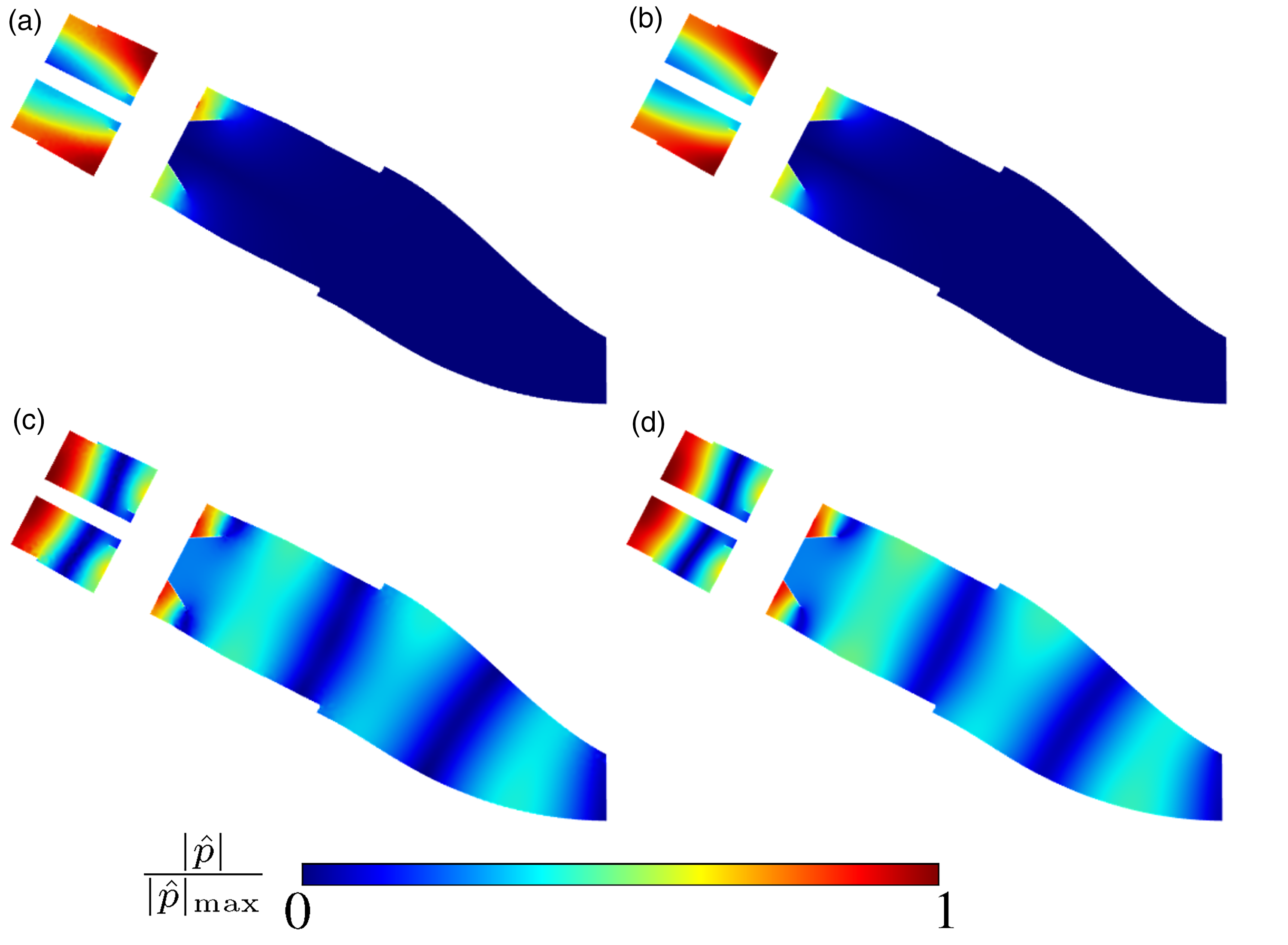
Comparison of selected mode shapes between the reference APE setup and the energetically consistent, homogeneous convective Helmholtz equation (hCHE-1). a) T1 mode APE. b) T1 mode hCHE-1. c) L3 mode APE. d) L3 mode hCHE-1.

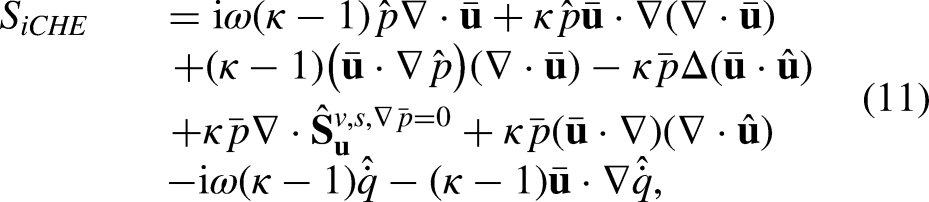
The root cause of this deviation lies in the interaction of the acoustic waves with the non-uniformity in the mean flow velocity. As discussed before, these interactions are represented by the volumetric source terms I - V within eq. (11). The first three source terms only depend on the solution variable of the convective Helmholtz equation and can thus be easily included in the numerical FEM framework. Their impact on the stability predictions is plotted in the stability map of Fig. 8. Here, the eigenvalues of the iCHE setup including each of the three source terms individually (I - III) and combined (I+II+III) are shown. The employed source terms are denoted in the index of iCHE. Again, the results of the APE are plotted for reference.

Figure 8.

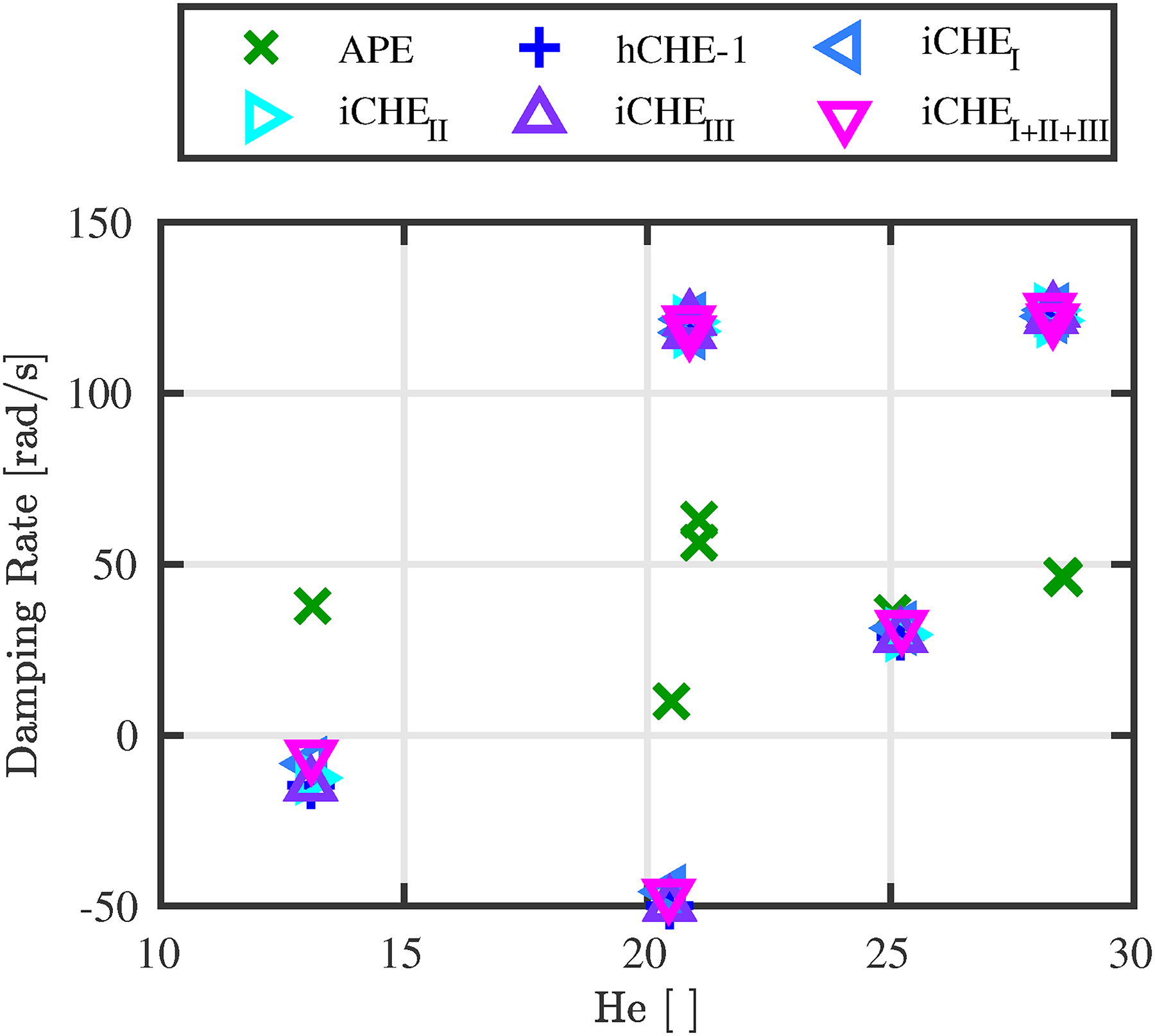
Stability map comparing the complex eigenfrequencies of the APE with those of the convective Helmholtz equation without (hCHE-1) and with (iCHE) different source terms describing the interactions between acoustics and flow non-uniformity. The index denotes the source terms applied to the iCHE.

Overall, the impact of the source terms is quite small. Analyzing the source terms reveals their dependency on the mean flow velocity’s divergence ( $\mathrm{\nabla }\cdot \overline{\mathbf{u}}$ ). In the present setup, this term is only significant in the vicinity of large temperature gradients. These regions coincide with the chemical reaction zone, which is substantial at the inner conical pilot flame guidance wall and extends further downstream into the transition zone (cf. Fig. 4). Particularly the transversal modes do not comprise pressure fluctuations in this region and are thus not affected by the source terms. With its large spatial extent, the flame can only be considered acoustically compact for low frequencies. For higher frequencies, the impact of the source terms can be assumed to vanish in an integral sense. Therefore, only for the first eigenfrequency a distinct impact of the source terms towards the reference solution is observed. It can thus be reasoned, that for the considered setup the source terms depending on the velocity fluctuations (IV and V) essentially determine the interactions between acoustics and non-uniform mean flow velocities and their impact on the stability predictions. However, these terms can not intrinsically be resolved without additional effort. This leads to the conclusion that the acoustically consistent hCHE setup generates significant errors when applied to arbitrary mean flow fields for thermoacoustic stability analyses (cf. Fig. 5 and 8).

When dropping the energetic consistency with the hCHE-2 setup by using the boundary conditions for stagnant fluids, the damping rates are expected to further deviate in comparison to the reference APE. However, while performing the underlying study with arbitrary mean flow fields, the results of the hCHE-2 were observed to match the results of the Helmholtz equation and the APE outstandingly well, when employing the energetically inconsistent boundary conditions of the Helmholtz equation. Figure 9 shows the comparison of the eigenvalues computed for the hCHE-2 setup with those of the APE and the HE.

Figure 9.

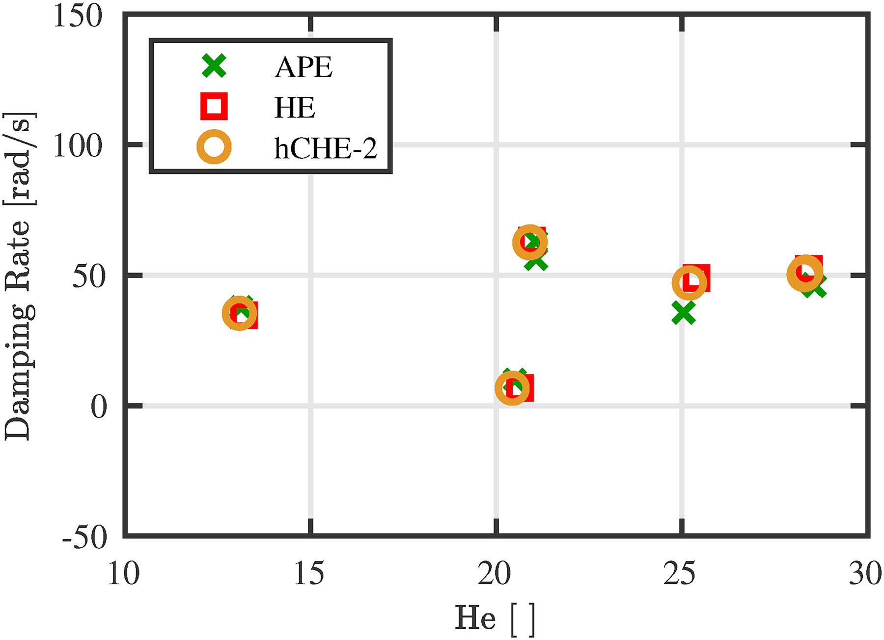
Stability map comparing the complex eigenfrequencies of the APE and the Helmholtz equation (HE) with those of the energetically inconsistent, homogeneous convective Helmholtz equation (hCHE-2). The inconsistency is achieved by applying the boundary conditions of the HE to the hCHE.

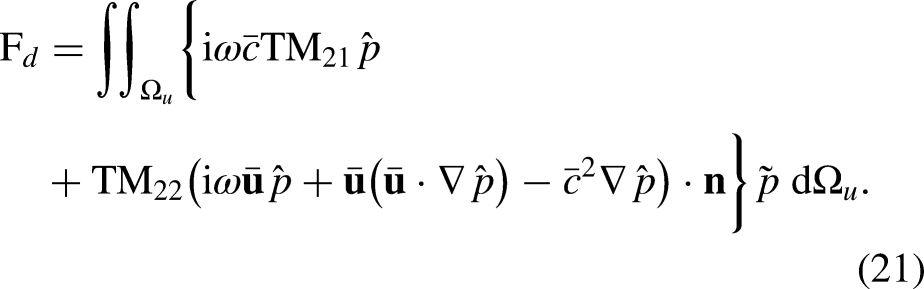
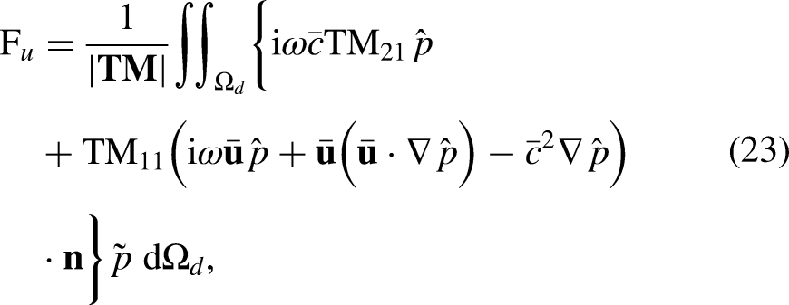
The observed results imply that the energetically inconsistent boundary flux of the convective Helmholtz equation compensates for the volume sources accounting for non-uniform mean flow fields on the RHS. In Appendix C light is shed on this phenomenon by comparing the boundary flux terms of the convective Helmholtz equation’s weak formulation (10) to the neglected volume source terms on the RHS, eq. (11). As a result, the following complete source term remains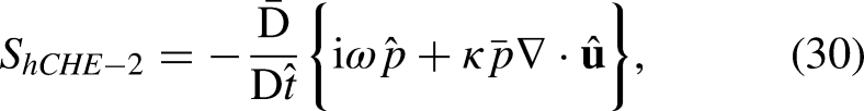

$$S_{hCHE-2}=-\frac{\overline{\mathrm{D}}}{\mathrm{D}\hat{t}}\{\mathrm{i}\omega \hat{p}+\kappa \overline{p}\mathrm{\nabla }\cdot \hat{\mathbf{u}}\},$$

(30)which is the material derivative of the acoustic energy equation for stagnant fluids without heat release. Supposing that a low Mach number mean flow does not significantly affect the mode shape, the mode shape approximately satisfies the linearized energy conservation of the Helmholtz equation. As a result, the overall resulting source term $S_{hCHE-2}$ vanishes. The assumption of source terms only having a marginal effect on the mode shape was made before by Culick ³³ for similarly investigating sources and their impact on the wave equation in a Lighthill analogy. It is further substantiated by comparing the mode shapes computed from APE, hCHE and the Helmholtz equation, which do not exhibit noticeable differences. Under the common assumption of negligible impact of the mean flow on the mode shape it may indeed be concluded that the erroneous fluxes approximately cancel the interaction mechanisms between acoustics and non-uniform mean flows. This may be interpreted with the help of the Gauss theorem: Sources and sinks due to the lacking mechanisms of acoustics and mean flow non-uniformity interactions introduce excitation or attenuation of the waves. This energetic discrepancy is simply transported out of the domain advectively due to the energetically inconsistent boundary conditions. This concept also works for the normal use case of a duct with uniform mean flow velocity. Due to the lack of acoustic sources, the energy advectively introduced at the inlet boundary is equally advected through the outlet boundary.

This analysis can be further substantiated by comparing the eigenvalues of the hCHE and the HE setups. The discrepancy in the damping rates between the hCHE-1 and hCHE-2 setup is a result of the erroneous energy fluxes at the boundaries of hCHE-2. Those energy fluxes compensate for the neglected volume sources. As a consequence one may expect an equivalent discrepancy between the Helmholtz setups HE and eiHE. With the same boundary conditions as used for the APE, the eiHE setup comprises erroneous energy fluxes, which are of the same magnitude as in the hCHE-2 setup. In fact, the eigenvalues of the eiHE setup are almost identical to those of the hCHE-1 setup, as visualized in the stability map of Fig. 10.

Figure 10.

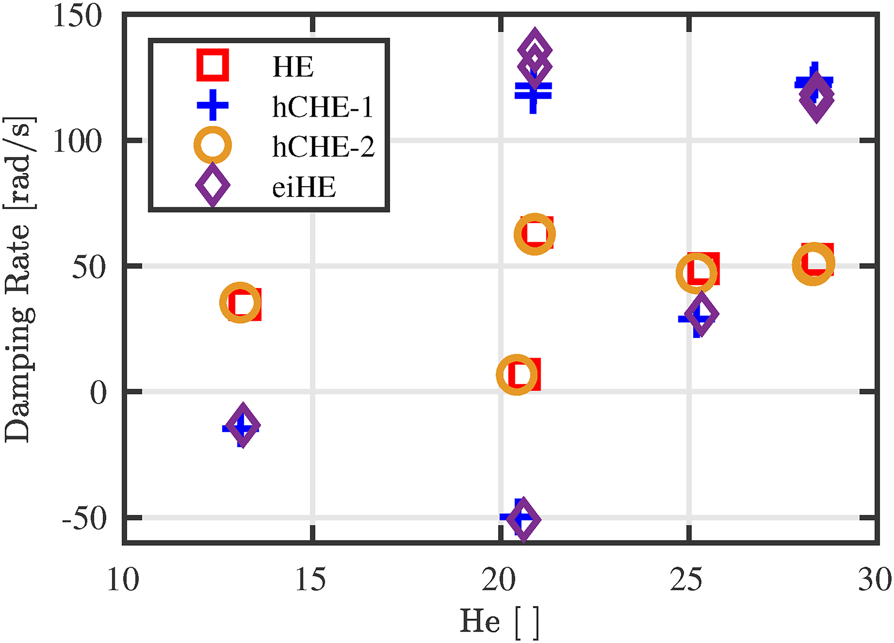
Stability map comparing the complex eigenfrequencies of the energetically consistent and inconsistent Helmholtz equations HE and eiHE to those of the homogeneous convective Helmholtz equation setups hCHE-1 and hCHE-2.

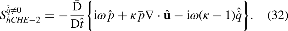
From the above analysis it may be inferred that the hCHE-2 setup actually corresponds to solving the acoustically consistent iCHE without the need to resolve the velocity fluctuations. To do so, eq. (16) has to be solved with boundary conditions energetically transformed for zero Mach number boundary conditions. ³¹ It can then be applied to arbitrary mean flow fields, even in the presence of flames. Also the impact of a fluctuating heat release can be included using the corresponding source terms of eq. (11), which modifies the RHS of eq. (16) to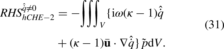

$$\begin{array}{rl}RH{S}_{hCHE-2}^{\hat{\dot{q}}\ne 0}& =-\int \int {\int }_V\{\mathrm{i}\omega (\kappa -1)\hat{\dot{q}}\\ & +(\kappa -1)\overline{\mathbf{u}}\cdot \mathrm{\nabla }\hat{\dot{q}}\}\tilde{p}\mathrm{d}V.\end{array}$$

(31)The validity can be proofed in the fashion of Appendix C. In this case, the deviation of the hCHE-2 setup compared to the iCHE in terms of the complete source term becomes

$$S_{hCHE-2}^{\hat{\dot{q}}\ne 0}=-\frac{\overline{\mathrm{D}}}{\mathrm{D}\hat{t}}\{\mathrm{i}\omega \hat{p}+\kappa \overline{p}\mathrm{\nabla }\cdot \hat{\mathbf{u}}-\mathrm{i}\omega (\kappa -1)\hat{\dot{q}}\}.$$

(32)This is the energy equation for zero Mach number flows including heat release fluctuations. Following the argument above, this term still approximately vanishes for $\hat{\dot{q}}\ne 0$ with the assumption of the mean flow not significantly altering the mode shape.

As a consequence, the hCHE-2 setup offers great benefits:

The equation of elliptic type is highly robust to solve with the FEM framework,

only solving one equation massively reduces the computational cost compared to the LEE or the APE and

in contrast to the Helmholtz equation the advection of acoustic waves is considered, which can lead to significant frequency drops for higher frequencies and Mach numbers.

Summary and Conclusions

In the present paper an acoustically consistent, inhomogeneous convective wave equation for the application in arbitrary mean flow fields is derived from the APE. Terms describing the interaction between acoustics and non-uniform mean flows are shifted to the right hand side (RHS). They act as sources on the acoustic waves advected by the mean flow velocity. For the use in FEM approaches, the weak formulation of the equation in frequency domain, referred to as inhomogeneous convective Helmholtz equation (iCHE), is derived. Additionally, suitable acoustic boundary conditions for frequency dependent impedances and transfer matrix couplings are presented. The errors introduced when applying the well-known homogeneous convective Helmholtz equation (hCHE) to arbitrary mean flow fields are investigated with a modal stability analysis of an industrial gas turbine combustion chamber. The results are compared to the APE and the Helmholtz equation for zero Mach numbers (HE). Applying the hCHE with energetically consistent boundary conditions (setup hCHE-1) to the setup leads to significant errors in terms of the predicted damping rates. These errors stem from the neglected interaction mechanisms of acoustics and mean flow gradients. The corresponding RHS source terms of the iCHE depending on the pressure fluctuations can easily be incorporated into the computations but do only have a minor effect on the stability predictions. The remaining source terms depending on the velocity fluctuations are crucial for the correct reproduction of acoustic wave propagation in non-uniform mean flow fields. However, their implementation is not feasible in a straightforward manner, which makes the regular energetically consistent, homogeneous convective Helmholtz equation not applicable to thermoacoustic stability analysis.

A way to circumvent this issue is the application of zero Mach number boundary conditions to the homogeneous convective Helmholtz equation (setup hCHE-2). These boundary conditions are normally applied to the Helmholtz equation for energetically consistent stability analyses. It is demonstrated that the erroneous boundary fluxes compensate for the source terms of the acoustically consistent, inhomogeneous convective Helmholtz equation while still considering the advection of acoustic waves. Consequently, this methodology represents a computationally efficient, highly robust and accurate approach for the stability prediction of large-scale thermoacoustic systems.