Generalized functions and acoustic analogy

Abstract

The aeroacoustic analogy is reviewed. The importance of generalized functions is demonstrated deriving Gauss like theorems in three and two dimensions. It is shown how the Dirac delta function plays an essential part in the theory of fundamental solutions (Green’s function). The concept of generalized derivatives as introduced by Farassat is derived in a consistent way for the time derivative and vector operations, for example gradient, divergence and curl. Applied to the wave equation, the impact of these operators when acting on surface distributions is presented. The compatibility conditions which apply at static and moving surfaces are derived in a unique manner. New source terms are found for the FW-H equation which steam from second order generalized derivatives, whereas all terms with the mass flux vector cancel out due to symmetry conditions. This procedure is validated by the derivation of the same result from the Lighthill equation directly and a term-by-term comparison with the Kirchhoff formula. Finally, it is shown how terms, containing the curvature of the integration surface, appear in the final solutions. The role of the $δ^{'} (f)$ factor in generating dipole as well as monopole sources is outlined. Essential knowledge provided from electromagnetic research is transferred to aeroacoustic theory. The vector wave equation is proposed instead of the scalar version to mitigate spurious noise effects.

Keywords

Acoustic analogy generalized derivative double layer curvature moving surface convective wave equation

Introduction

The aeroacoustic analogy was initiated by Lighthill¹ in the 1950s and extended by Ffowcs Williams and Hawkings² in the late 1960s with the incoorporation of boundary conditions. At that time the computational resources were poor and an important outcome of the theory were the scaling laws for monopole-, dipole- and quadrupole noise sources. Throughout this paper the abbreviation FW-H equation is used for Ffowcs Williams and Hawkings equation.

Intensive use of the acoustic analogy emerged from the growing computational capabilities. Farassat and Brentner^3–8 developed the foundations of propeller noise codes, based on mathematical theories of generalized functions. Thanks to Farassat, the power of these analytical tools became available not only to the mathematicians but also to the physicists and engineers. Together with Myers, Farassat derived the Kirchhoff formula^9,10 for a moving surface in an elegant manner. Today the numerical codes are regarded as well established and are applied without the need to know the underlying assumptions and principles.

Regardless of the success of the acoustic analogy, the author performed a literature review and found some open points for discussion.

- The derivation of the FW-H equation must start from the continuity and momentum equation. It fails, when the method is applied to the Lighthill equation directly.^4,11

- Kirchhoff formula and FW-H equation are both based on generalized functions and the wave operator for a quiescent acoustic free field. The difference is only attributed to the Lighthill term, but even so a comparison of the source terms is unsatisfactory.⁶

- Farassat mentioned the effect of surface curvature, but an integral formulation for applications is missing.

- The equations for the dipole noise source terms contain derivatives of the Dirac delta function restricted to the boundary surface. The equivalence to the dipole model as a distribution of two monopoles with opposite sign is not evident.

The application of generalized functions in physics comprises differential equations of first order. The propagation of shock waves is a well-known example. It is worth to mention, that in this case, the movement of the wave front is in straight lines along the normal of the surface with the speed of sound as a constant. In contrast, the imbedding procedure, used by Farassat and Myers¹⁰ for the FW-H equation and the Kirchhoff formula, is of second order. The discontinuity is selected artificially, and the velocity of the surface is not restricted to the normal direction alone but can move in tangential direction as well.

This paper is an attempt to collect the most important requirements in a unified manner and to emphasize the underlying principles with mathematical rigor but understandable for engineers. Thereby, novel approaches are outlined to solve the open points mentioned above.

Generalized functions

The mathematical operation with discontinuous functions like the unit step function (Heaviside function) or impulse function (Dirac delta function) is still not standard.¹² But in many situations, it is the natural way of processing. Think of the initial condition of a vibrating string, which is excited by a hammer blow. Another example is the deflection of a string at a single point which results in a discontinuous slope of the string. In this work, the use of the Heaviside function is demonstrated by the generalized theorems of divergence, gradient and curl and the importance of the Dirac delta function is shown in conjunction with the approach of the fundamental solution or Green’s function.

Throughout the paper $(y, τ)$ are used for source variables and $(x, t)$ are the observer variables for space and time.

A physical meaning for the Dirac delta function is only possible, when the integral with a continuous function is taken. The singular points of the discontinuous function can be resolved if the derivative operations are transferred to the continuous function. The continuous function is also called a regular function, whereas the discontinuous function is known as a singular function. In this paper, the Green’s function is understood as an example of a continuous function.

When the derivative is shifted from one function to the other function argument, the method of integration by parts is exploited. A peculiar principle in generalized function theory is the compactness assumption. At least one of the two involved functions must have bounded support and is zero outside the compact support region.

\int_{- \infty}^{+ \infty} \frac{\partial a (y)}{\partial y} b (y) d y = {a (y) b (y) |}_{- \infty}^{+ \infty} - \int_{- \infty}^{+ \infty} a (y) \frac{\partial b (y)}{\partial y} d y

(1)

The boundary is outside the support, therefore the first term on the right vanishes and equation (2) can always be used.

\int_{- \infty}^{+ \infty} \frac{\partial a (y)}{\partial y} b (y) d y = - \int_{- \infty}^{+ \infty} a (y) \frac{\partial b (y)}{\partial y} d y

(2)

This principle applies to temporal derivatives as well.

\int_{- \infty}^{+ \infty} \frac{\partial a (y, τ)}{\partial τ} b (y, τ) d y d τ = - \int_{- \infty}^{+ \infty} a (y, τ) \frac{\partial b (y, τ)}{\partial τ} d y d τ

(3)

If the limits of the integral are inside the support region, a layer of sources is taken at the boundary. Let’s apply this concept in conjunction with the multidimensional Heaviside function.

H (f) = {\begin{cases} 1 & f \geq 0 \\ 0 & f < 0 \end{cases}

(4)

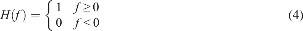
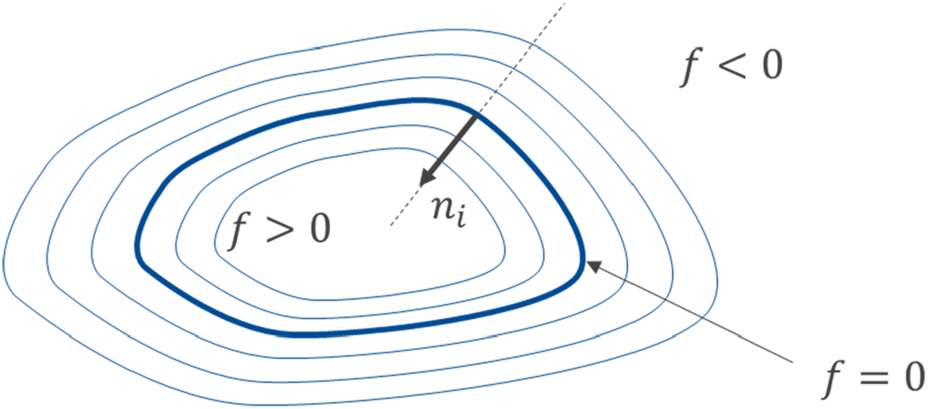
The variable $f$ is used to define a boundary surface where $f = 0$ , see Figure 1.

Figure 1.

Cross-sectional view of a three-dimensional region, bounded by means of potential field f.

The normal vector points in the direction of increasing $f$ and is normal to the surface.

n_{i} = \frac{\partial f}{{\partial y}_{i}}

(5)

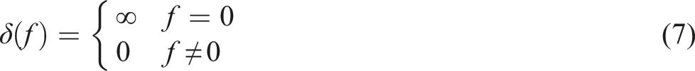
The derivative of the Heaviside function is the Dirac delta impulse.

δ (f) = \frac{\partial}{\partial f} H (f)

(6)

δ (f) = {\begin{cases} \infty & f = 0 \\ 0 & f \neq 0 \end{cases}

(7)

\int_{- \infty}^{+ \infty} δ (f) d f = 1

(8)

\int_{- \infty}^{+ \infty} δ (a f) d f = \int_{- \infty}^{+ \infty} \frac{1}{| a |} δ (f) d f = \frac{1}{| a |} \int_{- \infty}^{+ \infty} δ (f) d f

(9)

For equation (9) the variable was transferred from

f

→

a f

For the gradient, the chain rule applies:

\frac{\partial}{{\partial y}_{i}} H (f) = \frac{\partial}{\partial f} H (f) \cdot \frac{\partial f}{{\partial y}_{i}} = n_{i} \cdot δ (f) .

(10)

Note that this equation is valid in arbitrary dimension larger than $p = 1$ . In two-dimensional space the delta function symbolizes the boundary $f = 0$ . Figure 1 can again serve as an illustration, but now it shows the region directly rather than a cross-sectional view. The normal vector is in the plane and perpendicular to the boundary line. To make a distinction to the three-dimensional case, the normal vector should be renamed as $m_{i}$ rather than $n_{i}$ . In three dimensions, the delta function gives a closed boundary surface enclosing a volume and the vector $n_{i}$ is normal to the boundary surface. Usually, the variable $f$ is selected to gain a normalized vector, see equation (5). If not, the factor $a$ is eliminated in the product of equation (10) with help of equation (9).

Equation (2) is now considered in multi-dimensional space $p \geq 2$ with $i = 1 . . p$ .

For $p = 3$ we obtain

\int_{- \infty}^{+ \infty} \frac{\partial a (y_{i})}{\partial y_{i}} b (y_{i}) d V = - \int_{- \infty}^{+ \infty} a (y_{i}) \frac{\partial b (y_{i})}{\partial y_{i}} d V \begin{array}{l} ; & i = 1 . . 3 \end{array}

(11)

and for

p = 2

we get

\int_{- \infty}^{+ \infty} \frac{\partial a (y_{i})}{\partial y_{i}} b (y_{i}) d S = - \int_{- \infty}^{+ \infty} a (y_{i}) \frac{\partial b (y_{i})}{\partial y_{i}} d S \begin{array}{l} ; & i = 1 . . 2 . \end{array}

(12)

The function $b (y)$ can be replaced by the Heaviside function in equation (11). For the gradient of a scalar, the following equation is found for $p = 3$ .

\int_{- \infty}^{+ \infty} \frac{\partial a (y_{i})}{\partial y_{i}} H (f) d V = - \int_{- \infty}^{+ \infty} a (y_{i}) {\cdot n}_{i} \cdot δ (f) d V

(13)

Now the integration limits are adjusted to the volume on the left side and the enclosing boundary surface on the right side. When the normal vector is changed to point outwards, the negative sign will drop.

\int \frac{\partial a (y_{i})}{\partial y_{i}} d V = - \int a (y_{i}) {\cdot n}_{i} d S

(14)

In a further examination, the gradient is applied to the product of the two functions in equation (11). According to the product rule, the operation yields two terms which cancel out.

\int_{- \infty}^{+ \infty} \frac{\partial}{\partial y_{i}} (a (y_{i}) H (f)) d V = \int_{- \infty}^{+ \infty} \frac{\partial a (y_{i})}{\partial y_{i}} H (f) d V + \int_{- \infty}^{+ \infty} a (y_{i}) {\cdot n}_{i} \cdot δ (f) d V = \int \frac{\partial a (y_{i})}{\partial y_{i}} d V + \int a (y_{i}) {\cdot n}_{i} d S = 0

(15)

The same procedure can be performed for the divergence, time derivative and curl.

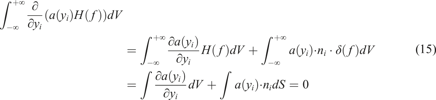
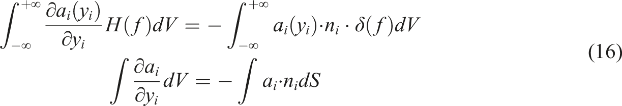
Divergence:

\int_{- \infty}^{+ \infty} \frac{\partial a_{i} (y_{i})}{\partial y_{i}} H (f) d V = - \int_{- \infty}^{+ \infty} a_{i} (y_{i}) {\cdot n}_{i} \cdot δ (f) d V \int \frac{\partial a_{i}}{\partial y_{i}} d V = - \int a_{i} {\cdot n}_{i} d S

(16)

\int_{- \infty}^{+ \infty} \frac{\partial}{\partial y_{i}} (a_{i} (y_{i}) H (f)) d V = \int_{- \infty}^{+ \infty} \frac{\partial a_{i} (y_{i})}{\partial y_{i}} H (f) d V + \int_{- \infty}^{+ \infty} a_{i} (y_{i}) {\cdot n}_{i} \cdot δ (f) d V = \int \frac{\partial a_{i} (y_{i})}{\partial y_{i}} d V + \int a_{i} (y_{i}) {\cdot n}_{i} d S = 0

(17)

Equation (16) is the famous divergence theorem in three-dimensional space, and it was deduced without the need of a coordinate system. The singular functions are not part of the final equation, but they were used as the intrinsic tool to provide the transition from the p-dimensional space to the (p-1)-dimensional space (hypersurface). Therefore, the theorem can be given for two-dimensional spaces or any higher dimension. In two dimensions the divergence theorem reads:

\int \frac{\partial a_{i}}{\partial y_{i}} d S = - \int a_{i} {\cdot m}_{i} d L \begin{array}{l} i = 1 . . 2 . \end{array}

(18)

Here, $d L$ is the arc length along the boundary line of the surface and $m_{i}$ is the unit normal vector tangential to the surface pointing inwards and which is perpendicular to the line segment $d L$ . Equation (18) is a remarkable achievement. It was deduced without the help of the Stokes theorem. Moreover, the Stokes theorem can be easily derived from equation (16). Usually, the equation is verified by comparing both sides of the equation for a particular coordinate system.^13,14 Kanwal¹⁵ also applied the derivative of the Heaviside function in two and three dimensions, but he used a coordinate system for the two-dimensional case that makes the more general interpretation as given here not obvious.

Time derivative:

It is supposed that the surface moves with velocity components $v_{i}$ . For the time derivative of the Heaviside function, the chain rule gives¹⁵

\frac{\partial}{\partial τ} H (f) = \frac{\partial}{\partial f} H (f) \cdot \frac{\partial f}{\partial τ} = {{- v}_{i} n}_{i} \cdot δ (f) .

(19)

In the next step, an observer moving with the surface is introduced. Derivatives seen by such an observer in the moving reference system are defined as

δ

derivatives. On the boundary we have the condition

f = 0

for all instances of time.

\frac{δ f}{δ τ} = 0 = \frac{\partial f}{\partial τ} + v_{i} \frac{\partial f}{\partial y_{i}} \begin{array}{l} ; & \frac{\partial f}{\partial τ} \end{array} = {{- v}_{i} n}_{i} = - v_{n}

(20)

The key point here is that only the normal component of the surface velocity enters the equation, because the gradient of $f$ points along the normal direction of the surface.¹³ Later it is shown that the normal component of the velocity is invariant to a change of the coordinate system. The mathematical principle of invariants is a very helpful methodology.¹⁶

In acoustic applications the moving surface may be assigned to a rotor blade or the wave front of a shock wave. For the latter case, the vector of the surface velocity has only one component along the normal direction with the speed of sound for all parts of the wave front.

With these preliminaries, we can proceed as with spatial derivatives.

\int_{- \infty}^{+ \infty} \frac{\partial a (y_{i}, τ)}{\partial τ} H (f) d V = \int_{- \infty}^{+ \infty} a (y_{i}, τ) {\cdot v}_{n} \cdot δ (f) d V

(21)

The integration limits are adjusted to the volume on the left side and the enclosing boundary surface on the right side.

\int \frac{\partial a (y_{i}, τ)}{\partial τ} d V = \int a (y_{i}, τ) {\cdot v}_{n} d S

(22)

As before, the derivative is applied to the product of the two functions.

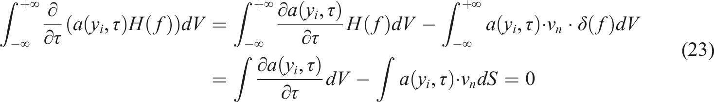
\int_{- \infty}^{+ \infty} \frac{\partial}{\partial τ} (a (y_{i}, τ) H (f)) d V = \int_{- \infty}^{+ \infty} \frac{\partial a (y_{i}, τ)}{\partial τ} H (f) d V - \int_{- \infty}^{+ \infty} a (y_{i}, τ) {\cdot v}_{n} \cdot δ (f) d V = \int \frac{\partial a (y_{i}, τ)}{\partial τ} d V - \int a (y_{i}, τ) {\cdot v}_{n} d S = 0

(23)

This equation is similar to the Reynold’s transport equation and can be used to demonstrate the conservation of a quantity.¹⁷

Equation (22) in two-dimensional space reads

\int \frac{\partial a (y_{i}, τ)}{\partial τ} d S = \int a (y_{i}, τ) {\cdot w}_{τ} d L,

(24)

where

w_{τ}

denotes the normal velocity on the boundary directed into the domain.

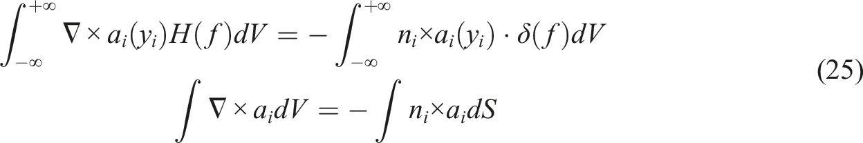
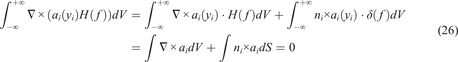
Curl:

\int_{- \infty}^{+ \infty} \nabla \times a_{i} (y_{i}) H (f) d V = - \int_{- \infty}^{+ \infty} n_{i} {\times a}_{i} (y_{i}) \cdot δ (f) d V \int \nabla \times a_{i} d V = - \int n_{i} {\times a}_{i} d S

(25)

\int_{- \infty}^{+ \infty} \nabla \times (a_{i} (y_{i}) H (f)) d V = \int_{- \infty}^{+ \infty} {\nabla \times a}_{i} (y_{i}) \cdot H (f) d V + \int_{- \infty}^{+ \infty} n_{i} {\times a}_{i} (y_{i}) \cdot δ (f) d V = \int \nabla \times a_{i} d V + \int n_{i} {\times a}_{i} d S = 0

(26)

The curl and cross product are not defined for higher dimensions. In two dimensions, the cross product can be regarded as a cross product with the unit normal of the plane. But the result depends on the choice to which side of the plane the normal vector points to. The curl and cross product can be given in tensor notation in three dimensions as follows¹³:

{(\nabla \times a)}_{i} = ε^{i j k} \frac{\partial a_{k}}{\partial y_{j}} {(a \times b)}_{i} = ε^{i j k} a_{j} b_{k} .

(27)

The antisymmetric tensor of third order is the Levi-Civita symbol. In two dimensions the curl becomes a scalar.

(\nabla \times a) = ε^{i j} \frac{\partial a_{j}}{\partial y_{i}} {(n \times b)}_{i} = ε^{i j} b_{j}

(28)

The following identity for the triple product rule might be useful.

a \cdot (b \times c) = ε^{i j k} a_{i} b_{j} c_{k} = (a \times b) \cdot c = ε^{i j k} {c_{i} a}_{j} b_{k}

(29)

Scalar product and cross product commute due to the properties of the Levi-Civita symbol. Two permutations are needed to switch between the two equations.

So far, useful equations were derived by mathematical rigor, which are exploited below for the definition of generalized derivatives. The fundamental solution is a further example, where important conclusions are gained with the help of the Dirac delta function. It is repeated here to remind the reader of some important concepts.

Fundamental solution and free field Green’s function

The simplest model of a source is a point source, which location is given by the Dirac delta function.

y_{0} = δ (y - y_{0})

(30)

If the equations are time dependent, an impulsive excitation at time $τ_{0}$ is used for the monopole source.

τ_{0} = δ (τ - τ_{0})

(31)

This monopole with source variables $(y_{0}, τ_{0})$ generates a field $G (x, t; y_{0}, τ_{0})$ with observer variables for space and time $(x, t)$ according to the linear partial differential operator $L$ .

L (G (x, t; y_{0}, τ_{0})) = δ (x - y_{0}) δ (t - τ_{0})

(32)

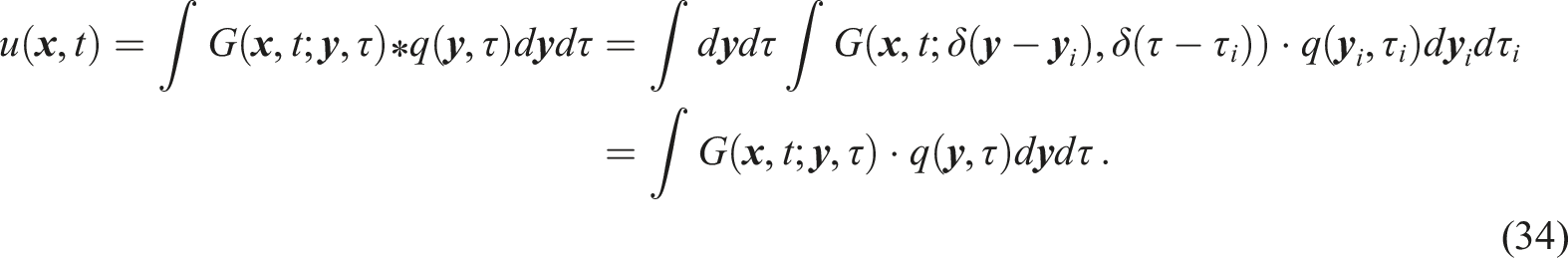
When solution $G (x, t; y_{0}, τ_{0})$ is known, the solution $u (x, t)$ for a distributed source field $q (y, τ)$ can be found by the principle of linear superposition.

L (u (x, t)) = q (x, t)

(33)

Let’s assume the following solution

u (x, t) = \int G (x, t; y, τ) * q (y, τ) d y d τ = \int d y d τ \int G (x, t; δ (y - y_{i}), δ (τ - τ_{i})) \cdot q (y_{i}, τ_{i}) d y_{i} d τ_{i} = \int G (x, t; y, τ) \cdot q (y, τ) d y d τ .

(34)

The symbol $*$ denotes the convolution product with respect to the space-time source domain. The inner integral over the dummy source space $(y_{i}, τ_{i})$ is simplified to a product with source variables given by the outer integral. The final integration sums up the reactions of the source distribution at the observer locations and observer time. The function $G (x, t; y_{0}, τ_{0})$ is called Green’s function.

If this equation is invoked in equation (33), the assumption of equation (34) is satisfied.

L (u (x, t)) = \int (L (G (x, t; y, τ))) * q (y, τ) d y d τ = \int δ (x - y) δ (t - τ) * q (y, τ) d y d τ = q (x, t)

(35)

For a convolution, the differential operator $L$ is applied to either of the function arguments only. But since the operator is defined in terms of observer variables, the Green’s function is the natural choice. Note again that the discontinuous functions appear only as one part within the integrant and are not present in the final solution.

In acoustic applications, the operator $L$ is the acoustic wave operator applied to a scalar $u$ which represents the acoustic density or acoustic pressure as received by an observer. The operator acts like a filter on the acoustic field (observer field) and is zero elsewhere except at locations and times where an acoustic source is present at that instant of time. The output of the filter is a measure of the source strength. The wave operator defines how the acoustic pressure fluctuations propagate, but it does not describe how the source is generated. Equation (33) is an inhomogeneous wave equation. The wave equation is entirely formulated with observer variables. However, the right part is interpreted as the source term. When this term is used to predict the radiated field adopting equation (34), the mathematical operations involved to calculate the term $q (y, τ)$ are inherent with respect to source variables. The Dirac delta function in equations (35) and (34) provides the mathematical bridge between both formulations of the source term $q$ in an elegant manner. Often the property of reciprocity is employed for the same purpose which makes the derivation more complex.

Before we proceed, the mathematical description of a monopole and dipole is reviewed. The interpretation of the acoustic sources in terms of point sources is of great importance for the physical understanding.

A monopole is equivalent to the free field Green’s function which is given in equation (36).

p_{M o n o p o l e} (x, t) = G (x, t; y_{0}, τ_{0}) = \frac{1}{4 π | x - y_{0} |} δ (t - τ_{0} - \frac{| x - y_{0} |}{c})

(36)

The speed of sound is denoted with $c$ . It is often convenient to express the free field Green’s function in the frequency domain. The Fourier transform of the Dirac delta function with time shift $t_{s}$ reads

\int_{- \infty}^{\infty} δ (t - t_{s}) \cdot e^{- j ω t} d t = 1 \cdot e^{- j ω t_{s}} \begin{array}{l} - \infty < ω < + \infty \end{array} .

(37)

It is seen that the spectrum is continuous with unit magnitude for all circular frequencies $ω$ . A phase shift is introduced due to the time shift $t_{s}$ . Equation (37) is applied to equation (36) to provide the following result

p_{M o n o p o l e} (x, y_{0}, ω) = G (x, y_{0}, ω) = \frac{e^{- j ω \frac{| x - y_{0} |}{c}}}{4 π | x - y_{0} |} \begin{array}{l} - \infty < ω < + \infty \end{array} .

(38)

It was implicitly assumed that source time and observer time are equal, and the time shift is accomplished by the phase delay given by the exponent of the numerator for each frequency component. This equation represents a continuous spectrum. The Dirac delta function serves as a model to capture the behavior at all frequencies. For physical applications, only the frequencies of interest might be used. This is a further demonstration how the artificial Dirac delta function is exploited to derive physical relations. Additional information about Fourier transform and discontinuous functions can be found in Olver.¹⁸

When the monopole is distributed over a surface $f$ , it is called a single layer.

p_{s i n g l e} (x, t) = \int a (f, τ) \cdot G (x, t; f, τ) d S d τ

(39)

A dipole is the arrangement of two point sources. One point source is placed with amplitude $+ q (τ)$ at $y_{1}$ and the second point source at $y_{2}$ with amplitude $- q (τ)$ . Each source radiates as a monopole into the free field. The total dipole field is thus given as

p_{D i p o l e} (x, t) = q (τ_{1}) \cdot G (x, t; y_{1}, τ_{1}) - q (τ_{2}) \cdot G (x, t; y_{2}, τ_{2}) .

(40)

The two sources are separated by a distance $2 ε$ along the normal direction $n$ .

\begin{array}{l} y_{1} = y_{0} + ε \cdot n & , & y_{2} = y_{0} - ε \cdot n \end{array}

(41)

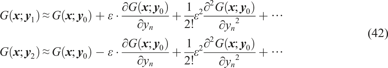
Nelson and Elliot¹⁹ applied a Taylor series expansion around $y_{0}$ to convert the difference in a derivative.

G (x; y_{1}) \approx G (x; y_{0}) + ε \cdot \frac{\partial G (x; y_{0})}{{\partial y}_{n}} + \frac{1}{2!} ε^{2} \frac{\partial^{2} G (x; y_{0})}{{\partial y}_{n}^{2}} + \dots G (x; y_{2}) \approx G (x; y_{0}) - ε \cdot \frac{\partial G (x; y_{0})}{{\partial y}_{n}} + \frac{1}{2!} ε^{2} \frac{\partial^{2} G (x; y_{0})}{{\partial y}_{n}^{2}} + \dots

(42)

Equation (40) can be rewritten as follows.

p_{D i p o l e} (x, t) = 2 \cdot ε \cdot q (τ_{0}) \cdot \frac{\partial G (x; y_{0})}{{\partial y}_{n}}

(43)

The product of the distance $2 ε$ with the source strength $q (τ)$ defines the dipole moment. Finally, for an ideal dipole the limit $ε \to 0$ must be taken. In that limit, the dipole moment remains constant.

d (τ_{0}) = 2 \cdot ε \cdot q (τ_{0})

(44)

Ehrenfried¹¹ performed the limit by introducing the scaling factor $1 / ε$ . Using L' Hôpital’s rule he found the formula

p_{D i p o l e} (x, t) = \lim_{ε \to 0} (\frac{d (τ_{1})}{2 ε} G (x; y_{1}) - \frac{d (τ_{2})}{2 ε} G (x; y_{2})) = d (τ_{0}) \cdot \frac{\partial G (x; y_{0})}{{\partial y}_{n}} .

(45)

This scaling property is inherent to the Dirac delta function, compare with equation (9). Howe²⁰ thus defined the dipole field in terms of Dirac delta functions.

q (τ_{1}) \cdot δ (y_{0} - ε \cdot n) - q (τ_{2}) \cdot δ (y_{0} + ε \cdot n) \approx - 2 \cdot ε \cdot q (τ_{0}) \cdot \frac{\partial}{{\partial y}_{n}} δ (y_{0})

(46)

When the integral with the Green’s function is calculated, the derivative in normal direction is switched to the Green’s function.

p_{D i p o l e} (x, t) = \int - G \cdot d (τ) \cdot \frac{\partial}{{\partial y}_{n}} δ (y_{0}) d V = d (τ) \cdot \frac{\partial G (x; y_{0})}{{\partial y}_{n}}

(47)

For dipoles distributed over a surface and with a dipole moment in normal direction, the equation of the double layer reads^15,21

p_{d o u b l e} (x, t) = \int d (f, τ) \cdot \frac{\partial G (x, t; f, τ)}{{\partial y}_{n}} d S d τ .

(48)

In equation (33) the expression for

q (y, τ)

can contain spatial derivatives. With the application of integration by parts or generalized function theory, mathematical operations that appear in

q (y, τ)

can be transferred to the source domain of the Green’s function. The widespread habit to move the operation from the source domain further to the observer domain of the Green’s function is seen critically by the author. The reader should be aware that this is only allowed due to the symmetry condition of the free field Green’s function. This paper tries to avoid such kinds of manipulations. An alternative procedure is given that results in an explicit formulation of monopoles and dipoles distributed on the boundary

f

of the source domain.

Generalized derivatives

Ffowcs Williams and Hawkings² were the first who introduced a data surface to propagate the acoustic field from that surface to the observer in the far field. The data surface discriminates the flow region from the acoustic region. The variables inside the flow region were set to the ones of a quiescent acoustic medium. This introduces an artifical discontinuity at the data surface. The method of integration by parts was used to find a differential equation. Nevertheless, the alternative procedure of generalized function technique was mentioned and even the final differential equation for the homogeneous wave equation was given but without derivation.²

The generalized function method is now well established and is applied in two ways. Some authors prefer the windowing technique,^11,22–24 where the variables are multiplied with the Heaviside function. Here the imbedding method of Farassat^4,10 is adopted, where the usual derivative operators are extended to include singular functions with discontinuities.

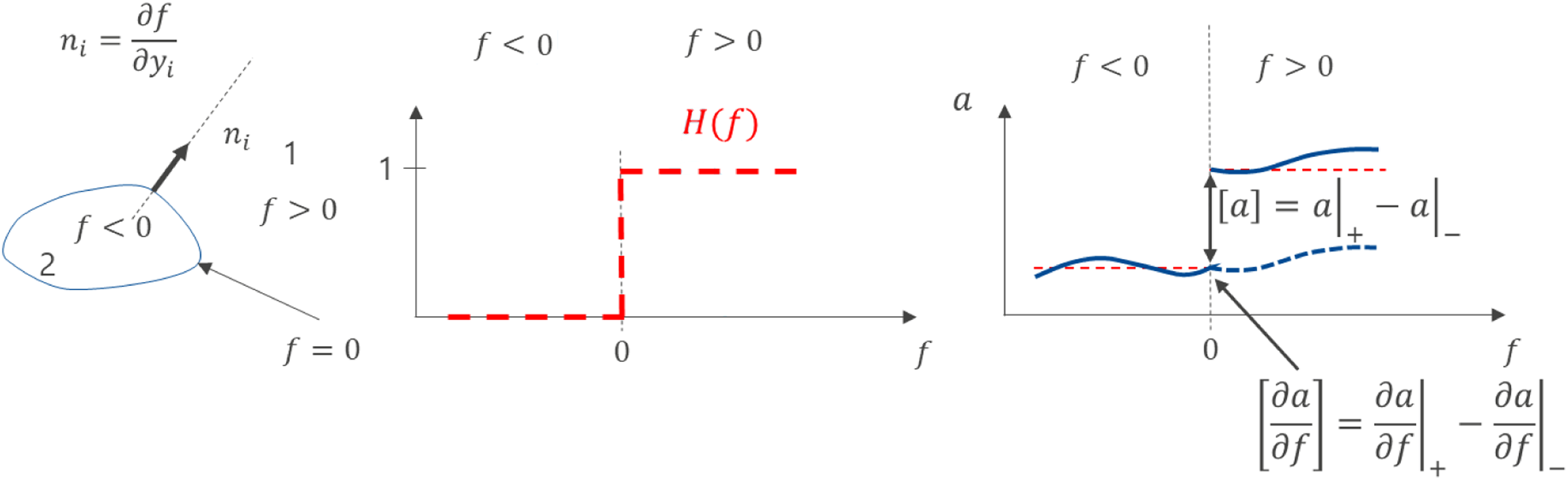
The surface $f = 0$ is described by general curvelinear (Gaussian) coordinates, where one of the basis vectors is the normal vector $n_{i}$ and the others are tangential to the surface, see for instance the Dupin coordinate system.^14,17 The curvelinear coordinates depend on the location at the surface. The variable $f$ then agrees with the normal coordinate, see left side of Figure 2. The discontinuity is along this variable $f$ where $f = 0$ . The Heaviside function models a unit step as shown in the middle of Figure 2. If the flow variable $a$ experiences a jump of magnitude $[a]$ , the unit step is scaled accordingly. The magnitude of the jump is the difference of the limits of the function $a$ aproaching the discontinuity from both sides.

[a] = {a |}_{+} - {a |}_{-}

(49)

Figure 2.

Data surface, left its definition in space, middle a discontinuity along the surface normal and right the abbreviation for the jump discontinuities.

The limit of the first derivative gives

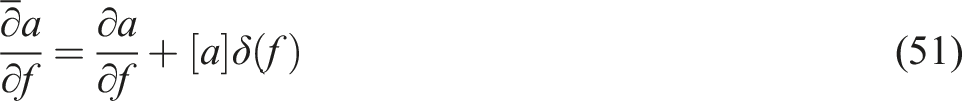
[\frac{\partial a}{\partial f}] = {\frac{\partial a}{\partial f} |}_{+} - {\frac{\partial a}{\partial f} |}_{-} .

(50)

It can be seen, that the following generalized derivative is the appropiate choice when operating with discontinous functions.

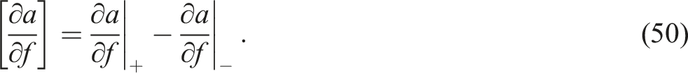
\frac{\bar{\partial} a}{\partial f} = \frac{\partial a}{\partial f} + [a] δ (f)

(51)

The bar over the operator indicates generalized derivation. The first term at the right is the regular part which is defined everywhere except at $f = 0$ . The second term is the singular part consisting of the jump magnitude and the Dirac delta function. This additional part is always added, where a discontinuity is present. It is important to note, that the singular part denoted with the square bracket, is only defined at $f = 0$ . The derivative of [a] with respect to $f$ is zero, as indicated in Figure 2 with the straight dotted red line on the left and right of the discontinuity in the right figure.

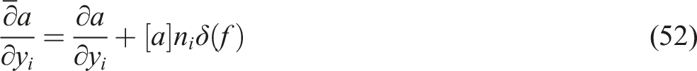
This result can be easily extended to three dimensions.

\frac{\bar{\partial} a}{{\partial y}_{i}} = \frac{\partial a}{{\partial y}_{i}} + [a] n_{i} δ (f)

(52)

The appearance of the normal vector in the singular part is an important property of the generalized derivative, when applied in higher dimensional space. This definition of equation (52) is linked to equation (15).

Differentiating with respect to $f$ is a derivative normal to the surface $f = 0$ . Furthermore, the derivative of the normal vector with respect to f is also zero, since the normal vector is not defined except on the surface. The conditions for normal derivatives are

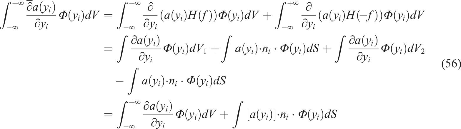
\begin{array}{l} \frac{\partial []}{\partial f} = 0 & , & \frac{\partial n_{i}}{\partial f} = 0 \end{array} .

(53)

The derivation of definition (52) is processed with the following four steps.

(1) The operation of interest is integrated with a test function $Φ (y_{i})$ and the operation is transfered to the test function.

\int_{- \infty}^{+ \infty} \frac{\bar{\partial} a (y_{i})}{\partial y_{i}} Φ (y_{i}) d V = - \int_{- \infty}^{+ \infty} a (y_{i}) \frac{\partial Φ (y_{i})}{\partial y_{i}} d V

(54)

(2) The Intergral is splitted in two parts $V_{1}$ and $V_{2}$ with the common boundary surface $δ (f)$ or $d S$ . Part 1 and part 2 are assigend to the domain $f > 0$ and $f < 0$ respectively, see Figure 2. To switch from part 1 to part 2, the sign of the argument of the Heaviside function is reversed.

- \int_{- \infty}^{+ \infty} a (y_{i}) \frac{\partial Φ (y_{i})}{\partial y_{i}} d V = - \int_{- \infty}^{+ \infty} a (y_{i}) H (f) \frac{\partial Φ (y_{i})}{\partial y_{i}} d V - \int_{- \infty}^{+ \infty} a (y_{i}) H (- f) \frac{\partial Φ (y_{i})}{\partial y_{i}} d V

(55)

(3) The operator is switched back from the test function to each volume part exploiting equation (15).

\int_{- \infty}^{+ \infty} \frac{\bar{\partial} a (y_{i})}{\partial y_{i}} Φ (y_{i}) d V = \int_{- \infty}^{+ \infty} \frac{\partial}{\partial y_{i}} (a (y_{i}) H (f)) Φ (y_{i}) d V + \int_{- \infty}^{+ \infty} \frac{\partial}{\partial y_{i}} (a (y_{i}) H (- f)) Φ (y_{i}) d V = \int \frac{\partial a (y_{i})}{\partial y_{i}} Φ (y_{i}) d V_{1} + \int a (y_{i}) {\cdot n}_{i} \cdot Φ (y_{i}) d S + \int \frac{\partial a (y_{i})}{\partial y_{i}} Φ (y_{i}) d V_{2} - \int a (y_{i}) {\cdot n}_{i} \cdot Φ (y_{i}) d S = \int_{- \infty}^{+ \infty} \frac{\partial a (y_{i})}{\partial y_{i}} Φ (y_{i}) d V + \int [a (y_{i})] {\cdot n}_{i} \cdot Φ (y_{i}) d S

(56)

(4) Finally, the test function appears as a factor in all terms and can be factored out to prove the assumption of equation (52)

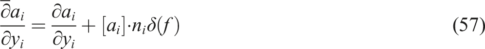
The same procedure can be carried out for the divergence, curl and time derivative. In step (3) the suitable equations have to be taken that are equations (17), (26), and (23) respectively. The results are as follows for the

Divergence:

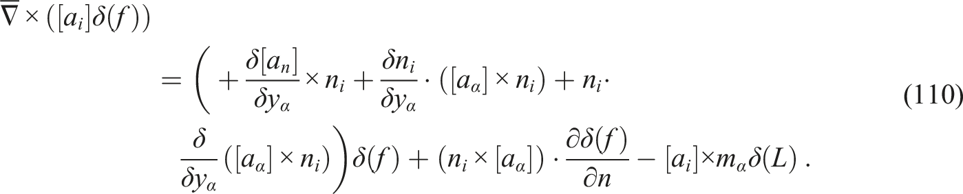
\frac{\bar{\partial} a_{i}}{{\partial y}_{i}} = \frac{\partial a_{i}}{{\partial y}_{i}} + [a_{i}] {\cdot n}_{i} δ (f)

(57)

Curl:

{\bar{\nabla} \times a}_{i} (y_{i}) = \nabla \times a_{i} + n_{i} \times [a_{i}] δ (f)

(58)

Time derivative:

\frac{\bar{\partial} a}{\partial τ} = \frac{\partial a}{\partial τ} - [a] v_{n} δ (f)

(59)

The higher order derivatives are likewise for spatial and temporal operators.

\frac{{\bar{\partial}}^{2} d_{i j}}{{{\partial y}_{j} \partial y}_{i}} = \frac{\bar{\partial}}{{\partial y}_{j}} (\frac{\bar{\partial} d_{i j}}{{\partial y}_{i}}) = \frac{\partial^{2} d_{i j}}{{{\partial y}_{j} \partial y}_{i}} + [\frac{\partial d_{i j}}{{\partial y}_{i}}] n_{j} δ (f) + \frac{\partial}{{\partial y}_{j}} ([d_{i j}] n_{i} δ (f))

(60)

A tensor of second order was used instead of a scalar to mention the connection with the Lighthill stress tensor. The Laplacian is gained setting $j = i$ .

\frac{{\bar{\partial}}^{2} a}{{{\partial y}_{i} \partial y}_{i}} = \frac{\bar{\partial}}{{\partial y}_{i}} (\frac{\bar{\partial} a}{{\partial y}_{i}}) = \frac{\partial^{2} a}{{{\partial y}_{i} \partial y}_{i}} + [\frac{\partial a}{{\partial y}_{i}}] n_{i} δ (f) + \frac{\partial}{{\partial y}_{i}} ([a] n_{i} δ (f))

(61)

\frac{{\bar{\partial}}^{2} a}{\partial τ^{2}} = \frac{\partial^{2} a}{\partial τ^{2}} - [\frac{\partial a}{\partial τ}] v_{n} δ (f) - \frac{\partial}{\partial τ} ([a] v_{n} δ (f))

(62)

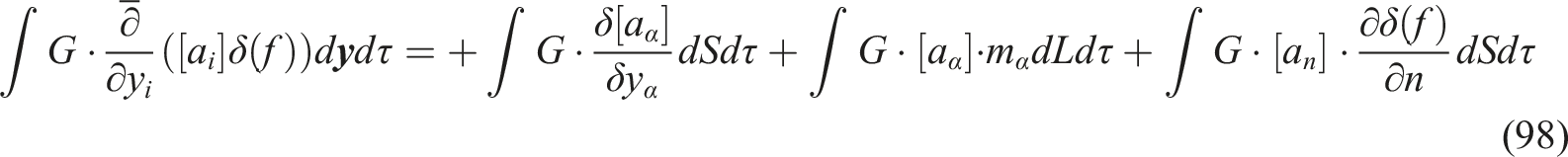
The second terms after the last equal signs in equations (60)–(62) contain the factor $δ (f)$ and represent monopole distributions. The factors in front of the Dirac-Delta functions are scalar quantities, which amplitudes vary over the surface. These scalars are the source strength of the monopole distributions.

Likewise, the third terms are related to the derivatives of the Dirac-Delta functions. Note, that the normal vector appears through the inner derivative

\frac{\partial}{{\partial y}_{i}} δ (f) = n_{i} δ^{'} (f) \begin{array}{l} , & {δ^{'} (f) = n}_{i} \frac{\partial}{{\partial y}_{i}} δ (f) . \end{array}

(63)

Further below it is shown that these distributions generate dipole layers on the surface but could give rise for monopole layers too.

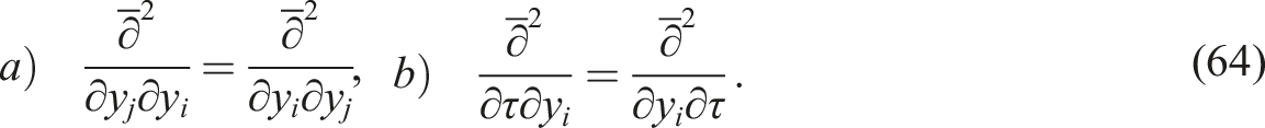
The terms in the square brackets are the jumps of the amplitude and the jumps of the first derivative on the data surface. It is now instructive to analyze the relations between these quantities which are known as compatibility conditions of the surface.^{15,21,25–27} The analysis is based on the following symmetry conditions

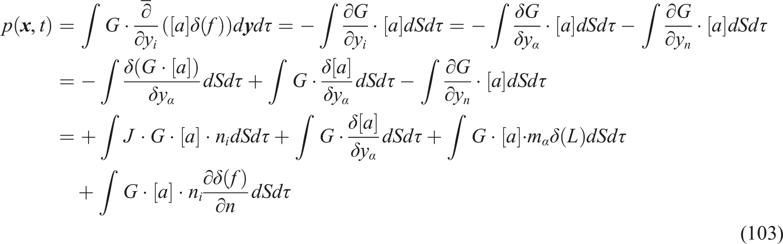
\begin{array}{l} \begin{array}{l} a) & \frac{{\bar{\partial}}^{2}}{{{\partial y}_{j} \partial y}_{i}} = \frac{{\bar{\partial}}^{2}}{{{\partial y}_{i} \partial y}_{j}} \end{array} & , & \begin{array}{l} b) & \frac{{\bar{\partial}}^{2}}{\partial τ {\partial y}_{i}} = \frac{{\bar{\partial}}^{2}}{\partial y_{i} \partial τ} \end{array} . \end{array}

(64)

The compatibility conditions are independent of the physical problem or the partial differential equations to be solved. Examining the first relation yields the identity

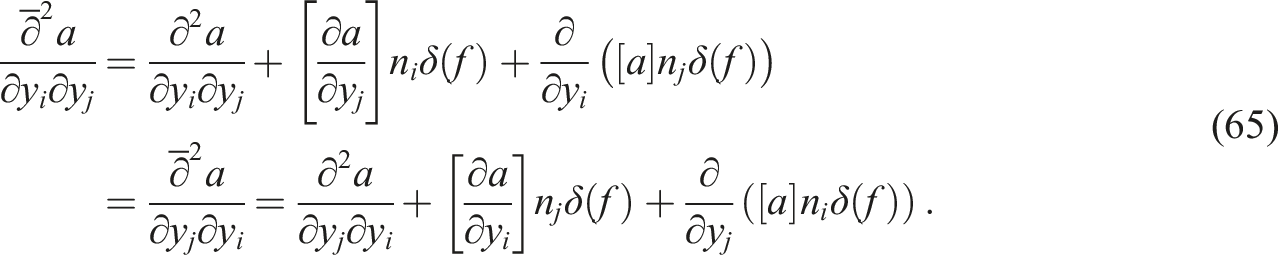
\frac{{\bar{\partial}}^{2} a}{{{\partial y}_{i} \partial y}_{j}} = \frac{\partial^{2} a}{{{\partial y}_{i} \partial y}_{j}} + [\frac{\partial a}{{\partial y}_{j}}] n_{i} δ (f) + \frac{\partial}{{\partial y}_{i}} ([a] n_{j} δ (f)) = \frac{{\bar{\partial}}^{2} a}{{{\partial y}_{j} \partial y}_{i}} = \frac{\partial^{2} a}{{{\partial y}_{j} \partial y}_{i}} + [\frac{\partial a}{{\partial y}_{i}}] n_{j} δ (f) + \frac{\partial}{{\partial y}_{j}} ([a] n_{i} δ (f)) .

(65)

It is assumed in an initial step, that the variable $a$ is continuous across the surface, then $[a] = 0$ and the terms with the round brackets vanish. Because the derivative operator commutes, the following symmetry relation is established.^15,21

[\frac{\partial a}{{\partial y}_{j}}] n_{i} = [\frac{\partial a}{{\partial y}_{i}}] n_{j} [\frac{\partial a}{{\partial y}_{j}}] = [\frac{\partial a}{{\partial y}_{i}}] n_{i} n_{j} = B n_{j}

(66)

To simplify notations, the given shorthand notations are used.

\begin{array}{l} A = [a] & ; & B = [\frac{\partial a}{{\partial y}_{i}}] n_{i} \end{array}

(67)

The final equation for the case $[a] \neq 0$ is provided in the Appendix.

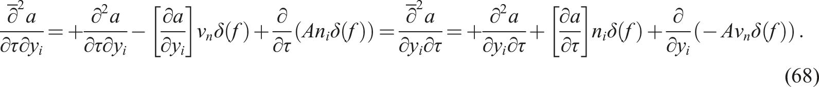
The same reasoning applies to the mixed temporal and spatial derivatives. From equation (126) we obtain the relation

\frac{{\bar{\partial}}^{2} a}{{\partial τ \partial y}_{i}} = + \frac{\partial^{2} a}{{\partial τ \partial y}_{i}} - [\frac{\partial a}{{\partial y}_{i}}] v_{n} δ (f) + \frac{\partial}{\partial τ} (A n_{i} δ (f)) = \frac{{\bar{\partial}}^{2} a}{{\partial y}_{i} \partial τ} = + \frac{\partial^{2} a}{{\partial y}_{i} \partial τ} + [\frac{\partial a}{\partial τ}] n_{i} δ (f) + \frac{\partial}{{\partial y}_{i}} (- A v_{n} δ (f)) .

(68)

For the case

A = 0

we get

- [\frac{\partial a}{{\partial y}_{i}}] v_{n} = [\frac{\partial a}{\partial τ}] n_{i} - [\frac{\partial a}{{\partial y}_{i}}] n_{i} v_{n} = [\frac{\partial a}{\partial τ}] = - B v_{n} .

(69)

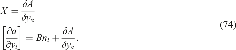
The terms with the round brackets in equation (68) can be expanded. The functions are restricted to the surface $δ (f)$ , therefore the differentiations must be operated in the moving reference frame which are known as the surface derivatives. The $δ$ operator is chosen for these derivatives. Greek letters are used to indicate surface coordinates rather than ambient spatial coordinates. The surface is two-dimensional, and the index goes from 1 to 2.

\frac{δ a}{{δ y}_{i}} = \frac{δ a}{δ y_{α}} \begin{array}{l} , & α = 1 . . 2 \end{array}

(70)

The expansion of both terms in equation (68) gives the following identities.

\frac{\partial}{\partial τ} (A n_{i} δ (f)) = \frac{δ A}{δ τ} n_{i} δ (f) + A \frac{δ n_{i}}{δ τ} δ (f) - A {v_{n} n}_{i} δ^{'} (f) \frac{\partial}{{\partial y}_{i}} (- A v_{n} δ (f)) = - \frac{δ A}{{δ y}_{α}} v_{n} δ (f) - A \frac{δ v_{n}}{{δ y}_{α}} δ (f) - A {v_{n} n}_{i} δ^{'} (f)

(71)

It is worth to mention, that each equation (71) constitutes three relations, one for the regular part and two for the singular terms with $δ (f)$ and $δ^{'} (f)$ . Singular functions cannot equal regular functions. Note that the terms with $δ^{'} (f)$ already fulfill the equivalence. The terms with $δ (f)$ yield

- [\frac{\partial a}{{\partial y}_{i}}] v_{n} + \frac{δ A}{δ τ} n_{i} + A \frac{δ n_{i}}{δ τ} = + [\frac{\partial a}{\partial τ}] n_{i} - \frac{δ A}{{δ y}_{α}} v_{n} - A \frac{δ v_{n}}{{δ y}_{α}} .

(72)

The terms in the brackets are replaced with the relations for the case $A = 0$ . Therefore, the terms are expanded with dummy factors $X$ and $Y$ to account for the condition $A \neq 0$ as well.

- B n_{j} v_{n} - X v_{n} + \frac{δ A}{δ τ} n_{i} + A \frac{δ n_{i}}{δ τ} = - B v_{n} n_{i} + Y n_{i} - \frac{δ A}{{δ y}_{α}} v_{n} - A \frac{δ v_{n}}{{δ y}_{α}}

(73)

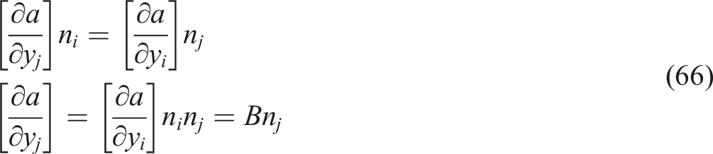
It is easily seen that the terms with $v_{n}$ are equal, when

X = \frac{δ A}{{δ y}_{α}} [\frac{\partial a}{{\partial y}_{i}}] = B n_{i} + \frac{δ A}{{δ y}_{α}} .

(74)

The equation states, that the jump of the spatial derivative can simply be decomposed into the normal component and the tangential components with respect to the surface or that the spatial derivatives are the same in the static ambient reference frame and the moving reference frame for the surface, see Morfey et al.²⁸.

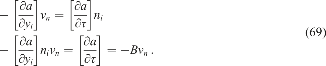
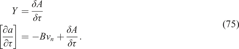
Accordingly for the terms with the normal vector, the equivalence in equation (73) is satisfied when

Y = \frac{δ A}{δ τ} [\frac{\partial a}{\partial τ}] = - B v_{n} + \frac{δ A}{δ τ} .

(75)

This equation states the transformation properties for the temporal derivative when changing between both reference systems. This becomes clear, when the term with the normal velocity is moved to the left side.

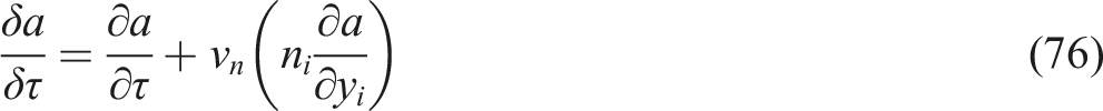
\frac{δ a}{δ τ} = \frac{\partial a}{\partial τ} + v_{n} (n_{i} \frac{\partial a}{{\partial y}_{i}})

(76)

It is demonstrated that only the normal gradient and normal velocity are accounted for.^24,28 The tangential velocity and the tangential gradients are ignored even when they exist. Grinfeld proposed to introduce a new operator $\dot{\nabla}$ for time derivatives on surfaces to sustain the tensor property of this operator. They are given here without proof for scalars and vectors in tensor notation.¹³ Note the difference between ambient spatial index $i$ in equation (77) and surface indices $α, β$ in equations (78) and (79).

\dot{\nabla} a = \frac{\partial a}{\partial τ} + v_{n} n_{i} \frac{\partial a}{\partial y_{i}}

(77)

This expression for scalars with ambient index agrees with equation (76) as derived in this paper. The reference point on the surface might change the position on the surface over time, which is accounted for in the following expression.¹³ This makes the expression invariant to the actual used parameterization of the surface.

\dot{\nabla} a = \frac{δ a}{δ τ} - v_{α} \frac{δ a}{δ y_{α}}

(78)

For covariant vectors, Grinfeld deduced the formula for vectors with respect to the moving surface

\dot{\nabla} a_{α} = \frac{δ a_{α}}{δ τ} - v^{β} \frac{δ a_{α}}{δ y_{β}} - (\frac{δ v^{β}}{δ y_{α}} - v_{n} B_{α}^{β}) a_{β} .

(79)

Variable $B_{α}^{β}$ is the curvature tensor of the surface. In case the wave equation is applied to the acoustic velocity, this vector equation must be applied.

Furthermore, when comparing the terms with factor $A$ in equation (72) the Thomas’ equation²⁷ is derived in a novel and simple way.

\frac{δ n_{i}}{δ τ} = - \frac{δ v_{n}}{{δ y}_{α}}

(80)

These terms vanish when the surface is an acoustic wave front in a homogeneous medium or the surface performs a translation with a uniform velocity vector.

Wave equations

This section contains material which was already presented by the author at the aero acoustic workshop “Strömungsschall in Luftfahrt, Fahrzeug- und Anlagentechnik“, held 23^th-24^th of November 2022 at DLR in Brunswick, Germany.

The theory of generalized functions is applied to derive the FW-H equation in a new fashion from the Lighthill equation and to provide a useful comparison with the Kirchhoff formula.

To ease the reading, the following abbreviations are used for the aero acoustic quantities.

\begin{array}{l} a = ρ - ρ_{0} & , & c^{2} a = p - p_{0} = p^{'} \end{array} b_{i} = ρ u_{i} d_{i j} = ρ u_{i} u_{j} - τ_{i j} + p^{'} δ_{i j}

(81)

With these notations, the equation for continuity of mass and momentum can be given.

\frac{\partial a}{\partial τ} + \frac{\partial b_{i}}{{\partial y}_{i}} = 0 \frac{\partial b_{i}}{\partial τ} + \frac{\partial d_{i j}}{{\partial y}_{j}} = 0

(82)

Both equations are combined to yield a wave equation for $a$ by eliminating the terms with $b_{i}$ . The first equation is derived with respect to time and the divergence is taken from the second equation. Subtracting the last from the first and expand both sides of the equation with a suitable term gives the Lighthill equation. The additional term on both sides is the second term on the left side and is incorporated in the Lighthill tensor on the right side.

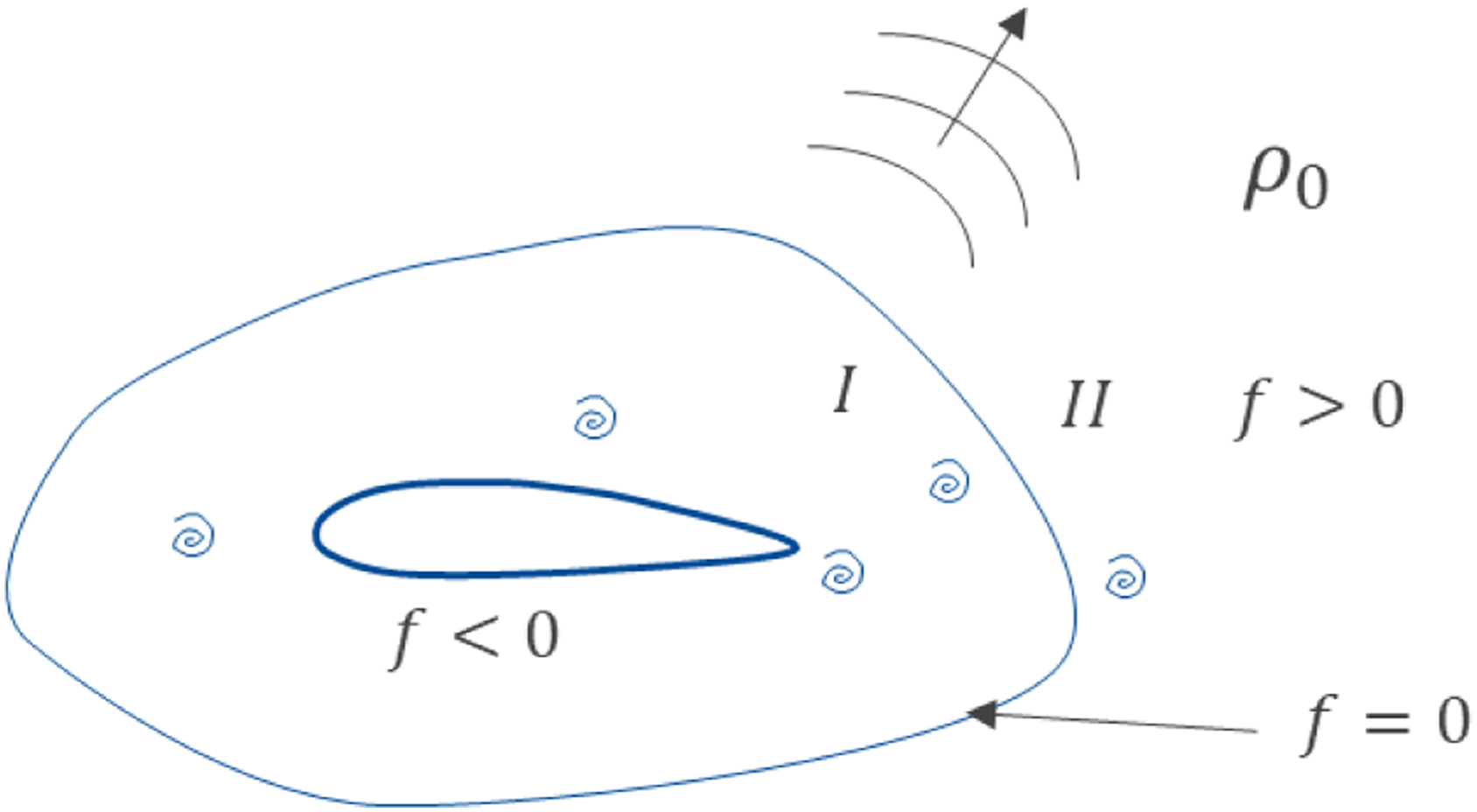
\begin{array}{l} \frac{\partial^{2} a}{\partial τ^{2}} {- c}^{2} \frac{\partial^{2} a}{\partial y_{i}^{2}} = \frac{\partial^{2} T_{i j}}{{\partial y_{j} \partial y}_{i}} & , & T_{i j} = ρ u_{i} u_{j} - τ_{i j} + (p^{'} {- c}^{2} a) δ_{i j} \end{array}

(83)

In the next step a data surface is introduced as proposed by Ffowcs Williams and Hawkings. The surface can be taken on the surface of a propeller blade, or it is shifted somewhat outside as pictured in Figure 3.

Figure 3.

Position of data surface, discriminating the flow region from quiescent acoustic region.

The variables inside the surface, where $f < 0$ , are set to zero.

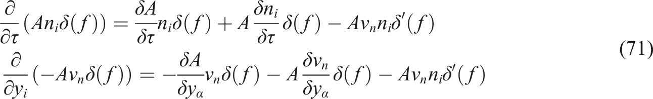
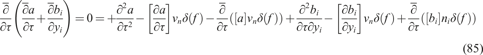
\begin{array}{l} a = 0 & , & \begin{array}{l} b_{i} = 0 & , & d_{i j} = 0 \end{array} \end{array}

(84)

Performing the same steps as for the Lighthill equation before, the equation of mass continuity is modified using generalized derivatives throughout

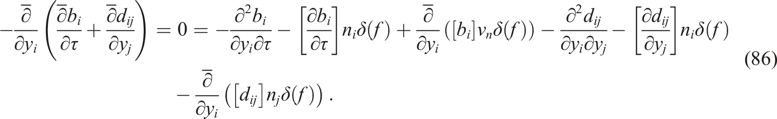
\frac{\bar{\partial}}{\partial τ} (\frac{\bar{\partial} a}{\partial τ} + \frac{\bar{\partial} b_{i}}{{\partial y}_{i}}) = 0 = + \frac{\partial^{2} a}{\partial τ^{2}} - [\frac{\partial a}{\partial τ}] v_{n} δ (f) - \frac{\bar{\partial}}{\partial τ} ([a] v_{n} δ (f)) + \frac{\partial^{2} b_{i}}{{\partial τ \partial y}_{i}} - [\frac{\partial b_{i}}{{\partial y}_{i}}] v_{n} δ (f) + \frac{\bar{\partial}}{\partial τ} ([b_{i}] n_{i} δ (f))

(85)

and the momentum equation follows accordingly

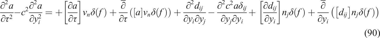
- \frac{\bar{\partial}}{\partial y_{i}} (\frac{\bar{\partial} b_{i}}{\partial τ} + \frac{\bar{\partial} d_{i j}}{{\partial y}_{j}}) = 0 = - \frac{\partial^{2} b_{i}}{{\partial y}_{i} \partial τ} - [\frac{\partial b_{i}}{\partial τ}] n_{i} δ (f) + \frac{\bar{\partial}}{\partial y_{i}} ([b_{i}] v_{n} δ (f)) - \frac{\partial^{2} d_{i j}}{{{\partial y}_{i} \partial y}_{j}} - [\frac{\partial d_{i j}}{{\partial y}_{j}}] n_{i} δ (f) - \frac{\bar{\partial}}{{\partial y}_{i}} ([d_{i j}] n_{j} δ (f)) .

(86)

This approach bears some new peculiarities, because the time derivative of the continuity equation is a generalized derivative as well as the divergence operation for the momentum equation. This is quite reasonable, since the third and sixth terms on the right side of both equations contain the surface fields with discontinuities. This was mentioned already by Farassat,^4,7 but was not executed in full consequence. Once generalized derivatives are required, the second and fifth terms on the right sides appear as new terms. These terms stem from second order derivatives and are well established when applied in conjunction with the homogeneous wave equation, as was done for the Kirchhoff method.^2,3,6,8,9

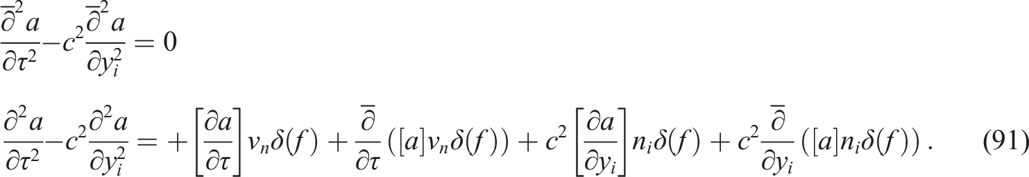
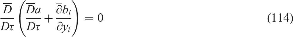
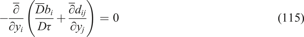
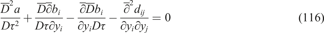
As mentioned before, generalized derivatives commute and all terms with $b_{i}$ cancel out. This leads to a separate equation and additional compatibility conditions which are provided in the Appendix. The utilization is deferred to the section devoted to the acoustic analogy with mean flow.

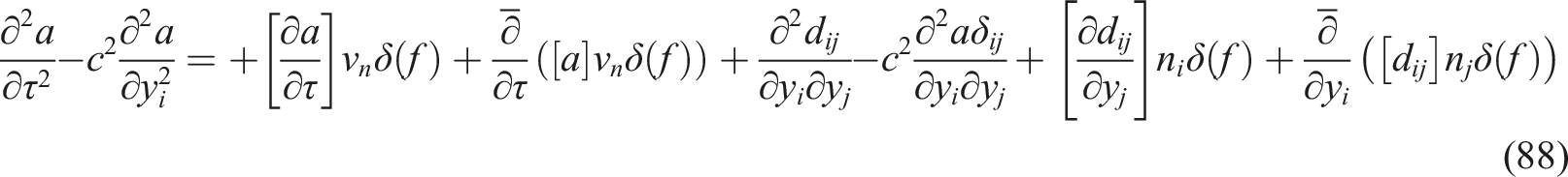
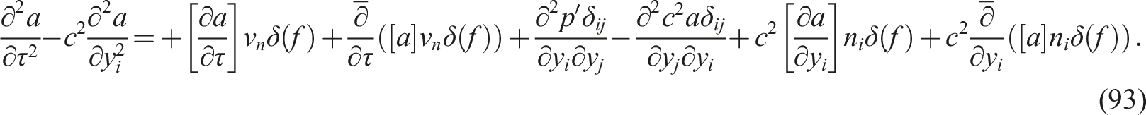
\frac{\partial^{2} b_{i}}{{\partial τ \partial y}_{i}} - [\frac{\partial b_{i}}{{\partial y}_{i}}] v_{n} δ (f) + \frac{\bar{\partial}}{\partial τ} ([b_{i}] n_{i} δ (f)) = + \frac{\partial^{2} b_{i}}{{\partial y}_{i} \partial τ} + [\frac{\partial b_{i}}{\partial τ}] n_{i} δ (f) - \frac{\bar{\partial}}{\partial y_{i}} ([b_{i}] v_{n} δ (f))

(87)

The combination of equations (85) and (86) gives the final result:

\frac{\partial^{2} a}{\partial τ^{2}} {- c}^{2} \frac{\partial^{2} a}{\partial y_{i}^{2}} = + [\frac{\partial a}{\partial τ}] v_{n} δ (f) + \frac{\bar{\partial}}{\partial τ} ([a] v_{n} δ (f)) + \frac{\partial^{2} d_{i j}}{{{\partial y}_{i} \partial y}_{j}} {- c}^{2} \frac{\partial^{2} a δ_{i j}}{{{\partial y}_{i} \partial y}_{j}} + [\frac{\partial d_{i j}}{{\partial y}_{j}}] n_{i} δ (f) + \frac{\bar{\partial}}{{\partial y}_{i}} ([d_{i j}] n_{j} δ (f))

(88)

The third and fourth term constitute the usual volume term with the Lighthill tensor. Equation (88) is an important result of the paper. It represents a modified version of the FW-H equation. This is confirmed as follows by the derivation of the same result from the Lighthill equation directly and a term-by-term comparison with the Kirchhoff formula.

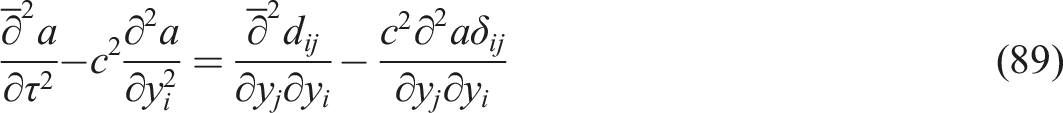
Starting the derivation from the Lighthill equation, the procedure is outlined here. All derivatives are taken as generalized derivatives. The second term is identical on both sides and the singular parts cancel each other. Therefore, only the regular derivative is utilized for both terms.

\frac{{\bar{\partial}}^{2} a}{\partial τ^{2}} {- c}^{2} \frac{\partial^{2} a}{\partial y_{i}^{2}} = \frac{{\bar{\partial}}^{2} d_{i j}}{{\partial y_{j} \partial y}_{i}} - \frac{c^{2} \partial^{2} {a δ}_{i j}}{{\partial y_{j} \partial y}_{i}}

(89)

The other terms are expanded, shifting the terms for the regular wave equation to the left side and the others to the right side.

\frac{\partial^{2} a}{\partial τ^{2}} {- c}^{2} \frac{\partial^{2} a}{\partial y_{i}^{2}} = + [\frac{\partial a}{\partial τ}] v_{n} δ (f) + \frac{\bar{\partial}}{\partial τ} ([a] v_{n} δ (f)) + \frac{\partial^{2} d_{i j}}{{{\partial y}_{i} \partial y}_{j}} - \frac{\partial^{2} c^{2} {a δ}_{i j}}{{\partial y_{j} \partial y}_{i}} + [\frac{\partial d_{i j}}{{\partial y}_{i}}] n_{j} δ (f) + \frac{\bar{\partial}}{{\partial y}_{i}} ([d_{i j}] n_{j} δ (f))

(90)

The result is identical to equation (88), thus both approaches are consistent. To the authors knowledge, this is the first time that this equivalence is shown. Farassat⁴ tried to achieve this, but the final proof was left open.

Finally, the homogeneous wave equation is examined. The second order derivatives were already presented with equations (61) and (62). The Kirchhoff formula reads

\frac{{\bar{\partial}}^{2} a}{\partial τ^{2}} {- c}^{2} \frac{{\bar{\partial}}^{2} a}{\partial y_{i}^{2}} = 0 \frac{\partial^{2} a}{\partial τ^{2}} {- c}^{2} \frac{\partial^{2} a}{\partial y_{i}^{2}} = + [\frac{\partial a}{\partial τ}] v_{n} δ (f) + \frac{\bar{\partial}}{\partial τ} ([a] v_{n} δ (f)) + c^{2} [\frac{\partial a}{{\partial y}_{i}}] n_{i} δ (f) + c^{2} \frac{\bar{\partial}}{{\partial y}_{i}} ([a] n_{i} δ (f)) .

(91)

This is almost identical to the new FW-H formulation. Exploiting the following simplification for the FW-H equation

d_{i j} = ρ u_{i} u_{j} - τ_{i j} + p^{'} δ_{i j} \approx p^{'} δ_{i j} \approx c^{2} a δ_{i j}

(92)

leads to the simplified FW-H equation

\frac{\partial^{2} a}{\partial τ^{2}} {- c}^{2} \frac{\partial^{2} a}{\partial y_{i}^{2}} = + [\frac{\partial a}{\partial τ}] v_{n} δ (f) + \frac{\bar{\partial}}{\partial τ} ([a] v_{n} δ (f)) + \frac{\partial^{2} p^{'} δ_{i j}}{{{\partial y}_{i} \partial y}_{j}} - \frac{\partial^{2} c^{2} {a δ}_{i j}}{{\partial y_{j} \partial y}_{i}} + c^{2} [\frac{\partial a}{{\partial y}_{i}}] n_{i} δ (f) + c^{2} \frac{\bar{\partial}}{{\partial y}_{i}} ([a] n_{i} δ (f)) .

(93)

The third and fourth terms cancel each other when $p^{'} δ_{i j} \approx c^{2} a δ_{i j}$ . These terms are related to heated jets²³ and thermoacoustic sources.²² The other terms can be assigned to the Kirchhoff formular directly.

Both methods fulfill the purpose to propagate the acoustic field from the data surface to the observer position. In this part II of the domain, where $f > 0$ (see Figure 3), the medium is at rest and the wave operator describes all physical processes. In an ideal configuration, the surface is chosen in such a way, that no noise source is present in that part II. The volume sources vanish then. All acoustic sources and flow dynamics are supposed to act in region I within the data surface. Any turbulent eddies passing the data surface are regarded as a violation of the model.^23,24 In these situations, the aerodynamic quantities on the surface must be isolated from the acoustic pressure or acoustic density to suppress spurious noise. The separation of acoustic wave quantities from aerodynamic quantities might be more appropriate in terms of the velocity vector. For this purpose, the wave equation can be formulated in terms of the velocity vector or the mass flux vector $b_{i}$ . See Griffiths²⁹ for a brief introduction into vector wave equations in the context of electrodynamics or Dunn³⁰ for an example of the acoustic wave operator applied to vectors.

Integral formulation

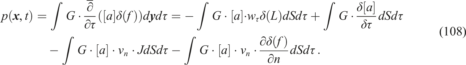
To get the acoustic pressure at the observer position, the source terms must be integrated with the free field Green’s function over the data surface, see equation (34). All terms with the factor $δ (f)$ in the equations (88) or (91) obviously represent monopole distributions on the data surface which are called single surface layer. It was already shown in equation (71) how the factor $δ^{'} (f)$ appears through the expansion of derivatives in conjunction with the round brackets which contain the factor $δ (f)$ .

It is demonstrated in this section that these $δ^{'} (f)$ factors give rise for dipole distributions or double surface layers and monopole distributions. The curvature of the data surface plays an important role in the generation of the monopole distributions. The properties of the source terms with $δ^{'} (f)$ can only be interpreted, when the integration with a continuous test function, the Green’s function, is performed. All these findings are ignored, when the derivative operator is transferred directly to the observer domain. This is only valid in the special case, when the spatial derivative is a divergence and performed on a vector which is normal to the surface.

The integration with the Green’s function is given for time derivates and the usual vector operations divergence, gradient and curl. That makes the procedure applicable to more general situations, where the variable of interest is a vector rather than a scalar like the acoustic density.

In the following it is shown, how the source terms of the FW-H equation and the Kirchhoff formula can be reformulated in terms of monopole and dipole distributions.

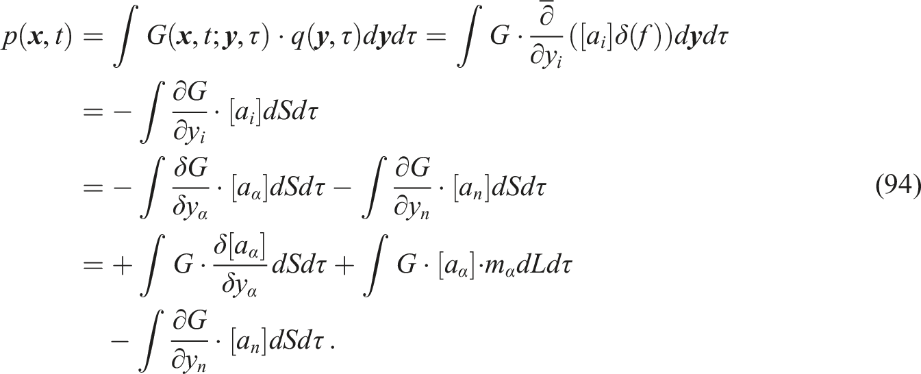
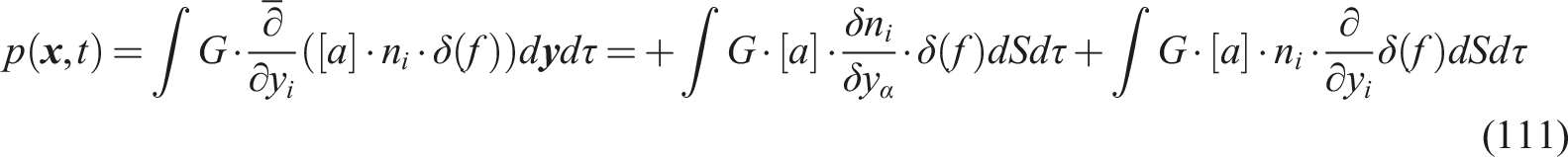
For the divergence operator, as it appears in the last term of equation (88) and equation (91), we get³¹

p (x, t) = \int G (x, t; y, τ) \cdot q (y, τ) d y d τ = \int G \cdot \frac{\bar{\partial}}{{\partial y}_{i}} ([a_{i}] δ (f)) d y d τ = - \int \frac{\partial G}{{\partial y}_{i}} \cdot [a_{i}] d S d τ = - \int \frac{δ G}{{δ y}_{α}} \cdot [a_{α}] d S d τ - \int \frac{\partial G}{{\partial y}_{n}} \cdot [a_{n}] d S d τ = + \int G \cdot \frac{δ [a_{α}]}{{δ y}_{α}} d S d τ + \int G \cdot [a_{α}] {\cdot m}_{α} d L d τ - \int \frac{\partial G}{{\partial y}_{n}} \cdot [a_{n}] d S d τ .

(94)

Please note, that the auxiliary vector $[a_{i}]$ denotes a substitution for

[a_{i}] = [a] n_{i}

(95)

when referred to equation (91) and

[a_{i}] = [d_{i j}] n_{j}

(96)

is used when associated with equation (88).

In the first step in equation (94), the derivative was transferred from the source term to the Green’s function. Then $δ (f)$ appears as a separated factor and the volume integral can be replaced by the surface integral. The second step consist in a splitting of the divergence into the surface component and normal component denoted with index $n$ . The surface component is transferred back by using equation (18). The second term with the line integral along $d L$ is zero, if $S$ is a closed surface. In both terms, $G$ appears as a factor giving rise for a monopole distribution. The normal gradient cannot be transferred back to the source, because the normal gradient does not exist for surface variables as mentioned before, see equation (53). The last term is just the representation of a dipole distribution with the dipole moment $[a_{n}]$ in normal direction. A new operator is defined for that integral to enable operational calculus.^15,32

\int G \cdot [a_{n}] \cdot \frac{\partial δ (f)}{\partial n} d S d τ = - \int \frac{\partial G}{{\partial y}_{n}} \cdot [a_{n}] d S d τ

(97)

The Green’s function appears as a factor in equation (98) and can be factored out in all terms to yield the operational equation (99) for the divergence of a surface layer.

\int G \cdot \frac{\bar{\partial}}{{\partial y}_{i}} ([a_{i}] δ (f)) d y d τ = + \int G \cdot \frac{δ [a_{α}]}{{δ y}_{α}} d S d τ + \int G \cdot [a_{α}] {\cdot m}_{α} d L d τ + \int G \cdot [a_{n}] \cdot \frac{\partial δ (f)}{\partial n} d S d τ

(98)

The operational equation is given as

\frac{\bar{\partial}}{{\partial y}_{i}} ([a_{i}] δ (f)) = \frac{δ [a_{α}]}{{δ y}_{α}} δ (f) + [a_{n}] \cdot \frac{\partial δ (f)}{\partial n} + [a_{α}] {\cdot m}_{α} δ (L) .

(99)

Only the second term on the right side radiates as a dipole. It is seen as an abuse by the author, if the surface derivative is not shifted back from the Green’s function to the source terms as was done in the last step in equation (94). In case of the Kirchhoff formula, the tangential components $[a_{α}]$ are zero and an error is avoided. However, for the FW-H equation the other monopole terms are effective and caused by the tensor $d_{i j}$ , see equation (96).

The gradient of a surface layer is a bit more challenging. It is necessary to follow the same steps as shown with the divergence operator. But we need to evaluate the surface divergence of a vector in three dimensions first.¹⁴

\int \frac{δ a_{i}}{δ y_{α}} d S = \int \frac{δ a_{α}}{δ y_{α}} d S + \int \frac{δ ((a_{i} \cdot n_{i}) \cdot n_{i})}{δ y_{α}} d S = - \int a_{α} {\cdot m}_{α} d L - \int J \cdot a_{i} \cdot n_{i} d S \begin{array}{l} i = 1 . . 2 \end{array}

(100)

The vector was decomposed into the tangential vectors and the normal vector component. For the tangential vectors

[a_{α}]

, equation (18) was exploited.

For the normal component, the product rule is applied. Taking the surface derivatives of the first factor, the scalar in the inner bracket, results in a tangential surface vector which gives no contribution, when the scalar product with the normal vector is performed. Only the derivative of the second factor contributes. The surface divergence of the normal vector is known to give the negative mean curvature $J$ , see Aris.¹⁷ The mean curvature^17,33 is the sum of the principal curvatures $κ_{α}$ .

\frac{δ n_{i}}{δ y_{α}} = - J = - (κ_{1} + κ_{2})

(101)

One can set the vector $a_{i}$ as a product of a scalar $Φ$ with a constant vector $c_{i}$ to find the useful relation.¹⁴

\int \frac{\partial Φ}{\partial y_{α}} d S = - \int Φ {\cdot m}_{i} d L - \int J \cdot Φ \cdot n_{i} d S \begin{array}{l} i = 1 . . 2 \end{array}

(102)

With these preliminaries, the gradient of a surface layer can be deduced.

p (x, t) = \int G \cdot \frac{\bar{\partial}}{{\partial y}_{i}} ([a] δ (f)) d y d τ = - \int \frac{\partial G}{{\partial y}_{i}} \cdot [a] d S d τ = - \int \frac{δ G}{{δ y}_{α}} \cdot [a] d S d τ - \int \frac{\partial G}{{\partial y}_{n}} \cdot [a] d S d τ = - \int \frac{δ (G \cdot [a])}{{δ y}_{α}} d S d τ + \int G \cdot \frac{δ [a]}{{δ y}_{α}} d S d τ - \int \frac{\partial G}{{\partial y}_{n}} \cdot [a] d S d τ = + \int J \cdot G \cdot [a] \cdot n_{i} d S d τ + \int G \cdot \frac{δ [a]}{{δ y}_{α}} d S d τ + \int G \cdot [a] {\cdot m}_{α} δ (L) d S d τ + \int G \cdot [a] \cdot n_{i} \frac{\partial δ (f)}{\partial n} d S d τ

(103)

The operational equation for the gradient of a surface layer is accordingly

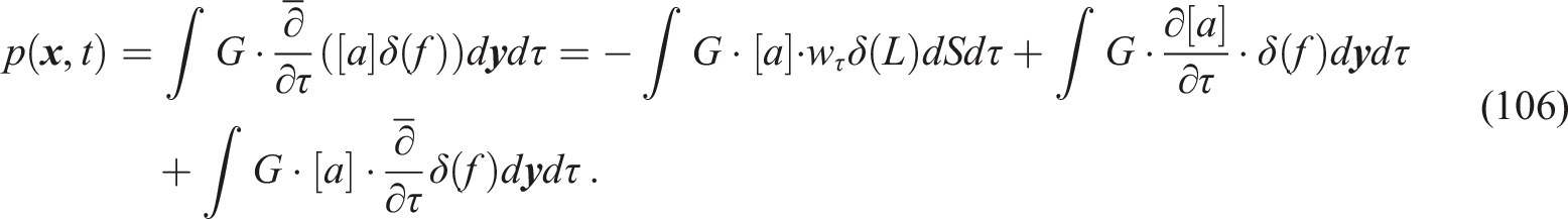
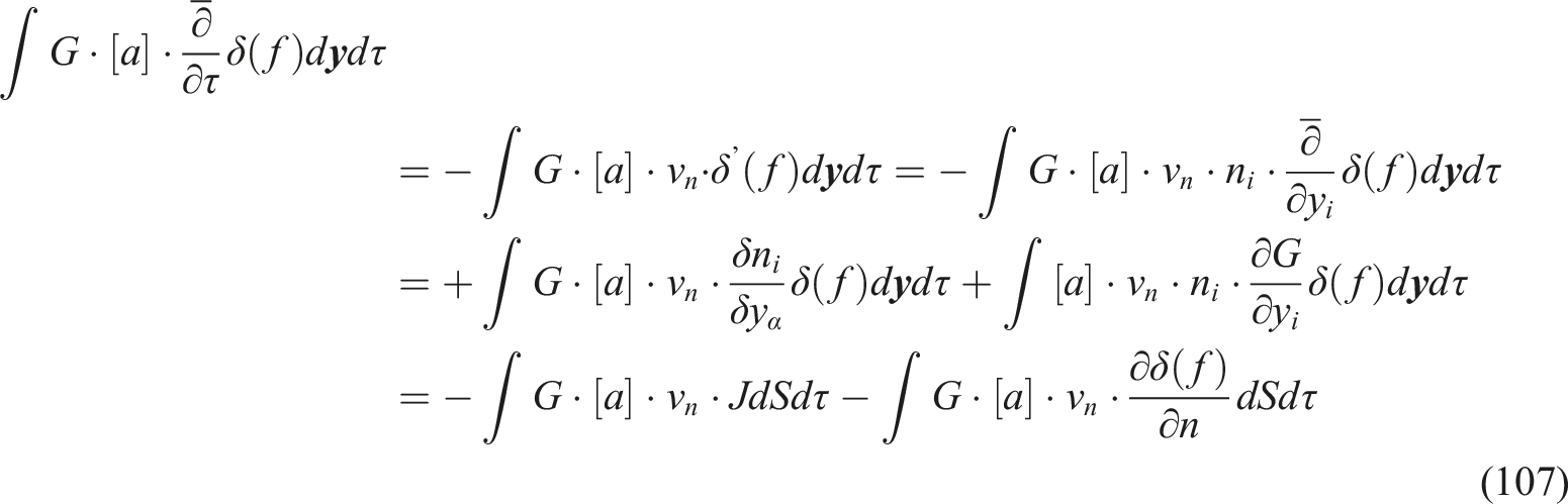
\frac{\bar{\partial}}{{\partial y}_{i}} ([a] δ (f)) = (J \cdot [a] \cdot n_{i} + \frac{δ [a]}{{δ y}_{α}}) δ (f) + [a] \cdot n_{i} \cdot \frac{\partial δ (f)}{\partial n} + [a] {\cdot m}_{α} δ (L) .

(104)

For the time derivative of a surface distribution, an additional equation is required.

From equations (20) and (63) it is found

\frac{\bar{\partial}}{\partial τ} δ (f) = - v_{n} δ^{'} (f) = {- v}_{n} n_{i} \frac{\bar{\partial}}{{\partial y}_{i}} δ (f) .

(105)

With the usual procedure, we achieve the formula

p (x, t) = \int G \cdot \frac{\bar{\partial}}{\partial τ} ([a] δ (f)) d y d τ = - \int G \cdot [a] {\cdot w}_{τ} δ (L) d S d τ + \int G \cdot \frac{\partial [a]}{\partial τ} \cdot δ (f) d y d τ + \int G \cdot [a] \cdot \frac{\bar{\partial}}{\partial τ} δ (f) d y d τ .

(106)

Further evaluation is performed on the last term.

\int G \cdot [a] \cdot \frac{\bar{\partial}}{\partial τ} δ (f) d y d τ = - \int G \cdot [a] \cdot v_{n} {\cdot δ}^{'} (f) d y d τ = - \int G \cdot [a] \cdot v_{n} \cdot n_{i} \cdot \frac{\bar{\partial}}{{\partial y}_{i}} δ (f) d y d τ = + \int G \cdot [a] \cdot v_{n} \cdot \frac{δ n_{i}}{{δ y}_{α}} δ (f) d y d τ + \int [a] \cdot v_{n} \cdot n_{i} \cdot \frac{\partial G}{{\partial y}_{i}} δ (f) d y d τ = - \int G \cdot {[a] \cdot v}_{n} \cdot J d S d τ - \int G \cdot [a] \cdot v_{n} \cdot \frac{\partial δ (f)}{\partial n} d S d τ

(107)

After the first row, the derivative is taken away from the Dirac delta function to the other factors. Note that the gradient in normal direction of the scalars $[a]$ and $v_{n}$ are zero and the surface or tangential derivative gives no contribution with the normal vector $n_{i}$ . Therefore, only the derivatives of $G$ and $n_{i}$ are to be considered.

Putting both equations together gives

p (x, t) = \int G \cdot \frac{\bar{\partial}}{\partial τ} ([a] δ (f)) d y d τ = - \int G \cdot [a] {\cdot w}_{τ} δ (L) d S d τ + \int G \cdot \frac{δ [a]}{δ τ} d S d τ - \int G \cdot {[a] \cdot v}_{n} \cdot J d S d τ - \int G \cdot [a] \cdot v_{n} \cdot \frac{\partial δ (f)}{\partial n} d S d τ .

(108)

The result for the operational time derivative of a surface layer is^15,26

\frac{\bar{\partial}}{\partial τ} ([a] δ (f)) = (+ \frac{δ [a]}{δ τ} - J \cdot [a] \cdot v_{n}) δ (f) + [a] \cdot v_{n} \cdot \frac{\partial δ (f)}{\partial n} - [a] {\cdot w}_{τ} δ (L) .

(109)

The derivation of the curl of a surface layer is beyond the scope of this paper. The relations of the equations (25) to (29) are exploited to give^34,35

\bar{\nabla} \times ([a_{i}] δ (f)) = (+ \frac{δ [a_{n}]}{{δ y}_{α}} \times n_{i} + \frac{δ n_{i}}{{δ y}_{α}} \cdot ([a_{α}] \times n_{i}) + n_{i} \cdot \frac{δ}{{δ y}_{α}} ([a_{α}] \times n_{i})) δ (f) + (n_{i} \times [a_{α}]) \cdot \frac{\partial δ (f)}{\partial n} - [a_{i}] {\times m}_{α} δ (L) .

(110)

It is noted, that for all operators except the divergence, the mean surface curvature must be included. The curvature appears in case of the divergence operator as well, but here it occurs two times and both parts cancel out. This is demonstrated as follows applying the procedure given by Kanwal.¹⁵

p (x, t) = \int G \cdot \frac{\bar{\partial}}{{\partial y}_{i}} ([a] \cdot n_{i} \cdot δ (f)) d y d τ = + \int G \cdot [a] \cdot \frac{δ n_{i}}{{δ y}_{α}} \cdot δ (f) d S d τ + \int G \cdot [a] \cdot n_{i} \cdot \frac{\partial}{{\partial y}_{i}} δ (f) d S d τ

(111)

So far, the first term depends on the surface curvature, but for the second term the derivative must be transferred to the other factors, resulting in two terms.

\int G \cdot [a] \cdot n_{i} \cdot \frac{\partial}{{\partial y}_{i}} δ (f) d S d τ = - \int G \cdot [a] \cdot \frac{δ n_{i}}{{δ y}_{α}} \cdot δ (f) d S d τ - \int [a] \cdot \frac{\partial G}{{\partial y}_{i}} \cdot n_{i} d S d τ

(112)

Thus, the first term cancels out and only the last term remains. This result is identical to equation (94) when the vector

a_{i}

has no tangential components and the surface is closed.

Acoustic analogy with mean flow

It was shown that a moving surface gives rise to the scalar $v_{n}$ , the normal velocity of the surface. This quantity appears then in the source terms of the FW-H equation (88) and the Kirchhoff equation (91). Curiously the tangential velocity is ignored.

Alternatively, the translational movement of a rigid body can be replaced by the rigid body at rest, but within a medium of uniform mean flow velocity $u_{i}$ . This scenario arises in wind tunnel tests. Here the data surface is identical to the surface of an airfoil. This means that the normal velocity $v_{n}$ of the body surface vanishes and the respective source terms must be replaced by terms with the velocity $u_{i}$ . Furthermore, the acoustic wave operator, as given on the left side in the equations (88) and (91), is modified to account for the mean flow effect. This change must affect the right side of the wave equation as well. Modified source terms are therefore expected. To calculate the far field radiation, the knowledge of the Green’s function with flow is required. But this is not covered here, and it is sufficient to restrict the analysis on the source terms. A comparison of the source terms for both treatments of the velocity provides further inside in the source generation mechanism.

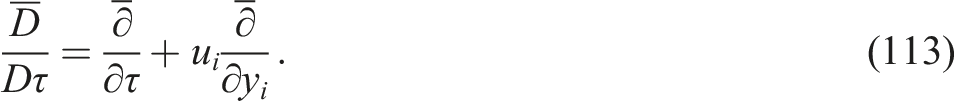
To incorporate the uniform background flow into the partial differential equation, it is sufficient to replace the partial derivative with respect to time by the convective derivative and to adopt generalized derivatives³⁶

\frac{\bar{D}}{D τ} = \frac{\bar{\partial}}{\partial τ} + u_{i} \frac{\bar{\partial}}{\partial y_{i}} .

(113)

If we start from the Lighthill equation (89), only the first term needs to be replaced and thus affects only the temporal derivatives of

a

in the first two rows of equation (90). When one starts instead with the mass continuity equation (85) and the momentum equation (86) the relations become

\frac{\bar{D}}{D τ} (\frac{\bar{D} a}{D τ} + \frac{\bar{\partial} b_{i}}{\partial y_{i}}) = 0

(114)

and

- \frac{\bar{\partial}}{\partial y_{i}} (\frac{\bar{D} b_{i}}{D τ} + \frac{\bar{\partial} d_{i j}}{\partial y_{j}}) = 0

(115)

respectively. Adding both equations gives the following result.

\frac{{\bar{D}}^{2} a}{D τ^{2}} + \frac{\bar{D} {\bar{\partial} b}_{i}}{D τ \partial y_{i}} - \frac{\bar{\partial} \bar{D} b_{i}}{\partial y_{i} D τ} - \frac{{\bar{\partial}}^{2} d_{i j}}{\partial y_{i} \partial y_{j}} = 0

(116)

The second and third term must cancel each other to proceed much like as before in equations (88) and (89). The equivalence can be shown my means of the compatibility conditions as given in the Appendix. The only difference is encountered by the first term, which is analyzed next.

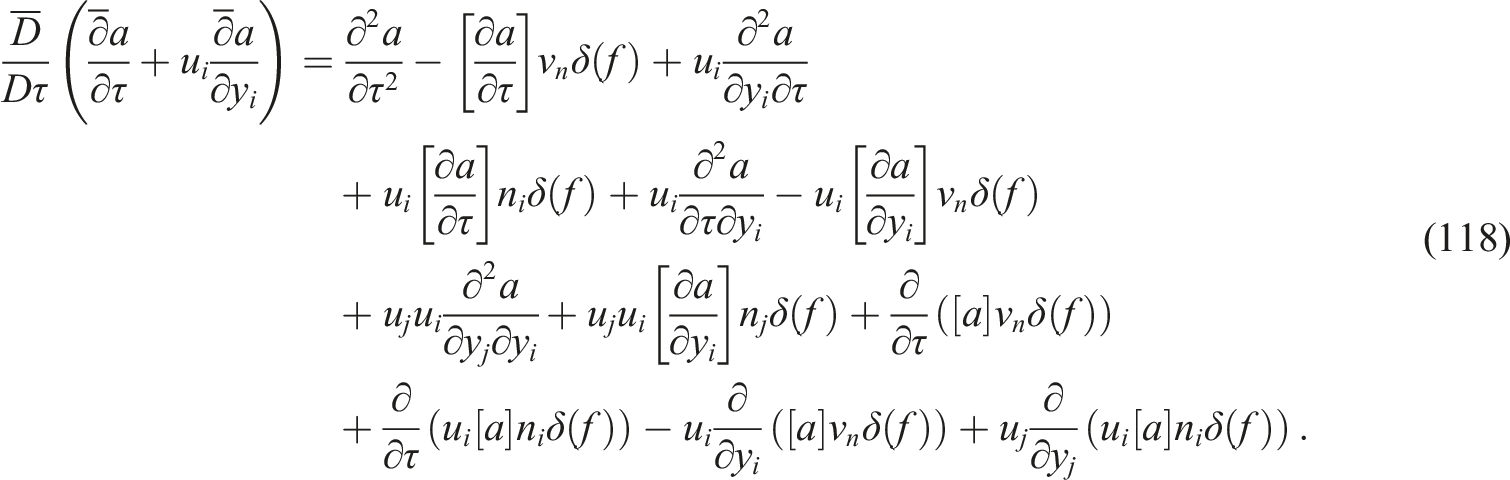
The first term in equation (116) is processed in two steps.

\frac{\bar{D} a}{D τ} = \frac{\partial a}{\partial τ} - [a] v_{n} δ (f) + u_{i} \frac{\partial a}{\partial y_{i}} + u_{i} [a] n_{i} δ (f)

(117)

The second step gives the following interesting result

\frac{\bar{D}}{D τ} (\frac{\bar{\partial} a}{\partial τ} + u_{i} \frac{\bar{\partial} a}{\partial y_{i}}) = \frac{\partial^{2} a}{{\partial τ}^{2}} - [\frac{\partial a}{\partial τ}] v_{n} δ (f) + u_{i} \frac{\partial^{2} a}{{\partial y}_{i} \partial τ} + u_{i} [\frac{\partial a}{\partial τ}] n_{i} δ (f) + u_{i} \frac{\partial^{2} a}{{\partial τ \partial y}_{i}} - u_{i} [\frac{\partial a}{{\partial y}_{i}}] v_{n} δ (f) + u_{j} u_{i} \frac{\partial^{2} a}{{{\partial y}_{j} \partial y}_{i}} + u_{j} u_{i} [\frac{\partial a}{{\partial y}_{i}}] n_{j} δ (f) + \frac{\partial}{\partial τ} ([a] v_{n} δ (f)) + \frac{\partial}{\partial τ} (u_{i} [a] n_{i} δ (f)) - u_{i} \frac{\partial}{{\partial y}_{i}} ([a] v_{n} δ (f)) + u_{j} \frac{\partial}{{\partial y}_{j}} (u_{i} [a] n_{i} δ (f)) .

(118)

The regular terms constitute the modified wave operator together with the Laplacian from equation (90) to give the inhomogeneous wave equation with uniform mean flow.

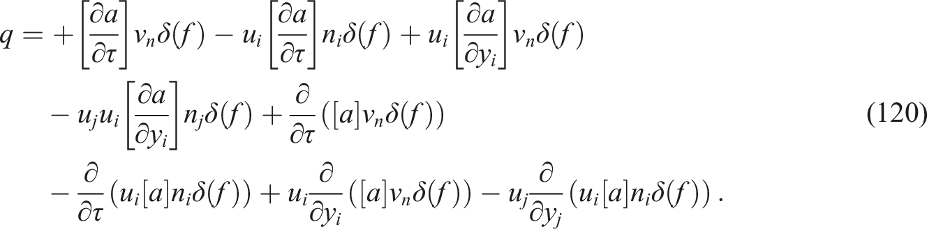
\frac{\partial^{2} a}{{\partial τ}^{2}} + 2 \cdot u_{i} \frac{\partial^{2} a}{{\partial y}_{i} \partial τ} + u_{j} u_{i} \frac{\partial^{2} a}{{{\partial y}_{j} \partial y}_{i}} {- c}^{2} \frac{\partial^{2} a}{\partial y_{i}^{2}} = q

(119)

The new source terms, which replace the first and second term on the right of equation (90), are

q = + [\frac{\partial a}{\partial τ}] v_{n} δ (f) - u_{i} [\frac{\partial a}{\partial τ}] n_{i} δ (f) + u_{i} [\frac{\partial a}{{\partial y}_{i}}] v_{n} δ (f) - u_{j} u_{i} [\frac{\partial a}{{\partial y}_{i}}] n_{j} δ (f) + \frac{\partial}{\partial τ} ([a] v_{n} δ (f)) - \frac{\partial}{\partial τ} (u_{i} [a] n_{i} δ (f)) + u_{i} \frac{\partial}{{\partial y}_{i}} ([a] v_{n} δ (f)) - u_{j} \frac{\partial}{{\partial y}_{j}} (u_{i} [a] n_{i} δ (f)) .

(120)

Without mean flow

u_{i} = 0

, we receive back the ordinary formulas with two source terms only, the first and fifth one. Whereas with mean flow, the normal velocity is set to

v_{n} = 0

. This means, that the rigid body or airfoil is at a fixed position and all terms with

v_{n}

vanish. But we can replace

u_{i} n_{i}

according to

u_{i} n_{i} {= u}_{n} = {- v}_{n} .

(121)

With this condition, the ordinary source terms are substituted one by one with new ones, as the first by the second and the fifth by the sixth respectively. The third and the seventh term are cross terms and vanish in both situations.

However, the fourth and the last terms are an essential manifestation of a new source mechanism. The different formulation of the wave operator causes an adaptation of the source terms. The fourth term is of pure monopole type. The last term is evaluated as the gradient of a scalar surface distribution according to equation (104). The source is of monopole type and dipole type. The surface curvature contributes to the monopole part. Both terms, fourth and eighth, are supposed to be effective in the nose region of the rotor blade.

This is a powerful demonstration, where the suitable mathematical framework provides meaningful physical insight. In this novel approach the knowledge of the Green’s function is not required. The equivalence of the normal mean flow and the normal surface velocity might give a better understanding of the mathematical equations. The acoustic analogy models the acoustic wave propagation with suitable source terms. A numerical flow simulation provides the field quantities for the acoustic source terms as required by the acoustic analogy. The boundary condition of the flow field is accounted for by the flow simulation but not by the acoustic source terms. The acoustic source terms satisfy the acoustic boundary condition at the data surface.

Conclusions

This paper collects the most important foundations of the acoustic analogy in a unified treatment. The mathematical derivations are based on a few underlying principles, but are applied with mathematical rigor to ease the understanding for engineers. The FW-H equation is modified in a way that it can be derived from the Lighthill equation directly. The achieved term by term comparison with Kirchhoff formula might be helpful in the interpretation of results from acoustic predictions. Knowing the underlying assumptions of the acoustic analogy is seen as an essential requirement to deal with spurious noise and other limitations in engineering applications.

It was shown that the operators acting on surface discontinuities obey special mathematical rules. To distinguish these surface fields from other fields it is recommended to provide a unique notation like the square brackets [ ] as was done in this paper for such fields. It was demonstrated that the $δ^{'} (f)$ terms give rise for dipole distributions or double surface layers and monopole distributions. The curvature of the data surface plays an important role in the generation of the monopole distributions. Moving surfaces with discontinuities in the field quantities are an outstanding feature of the acoustic analogy. The challenging time derivative on a moving surface was deduced in a unique fashion exploiting symmetry rules for the compatibility conditions on the surface.

The source distributions on the data surface represent virtual sources replacing the one in the flow field. It is important to note, that the free field Green’s function is used for these virtual sources. The acoustic radiation to the observer positions is performed in a free field with no flow and any physical surfaces are absent. The distribution of virtual sources accounts for reflections at physical surfaces in the flow region. Shifting the data surface away from physical surfaces is beneficial to comply with the assumptions of the theory. But an interpretation of the virtual sources is more realistic, if the data surface coincidences with a physical surface, for example the surface of an airfoil.

The nose region of the rotor blade is assumed to be an effective source area. This is supported by the occurrence of the extrema of the normal surface velocity $v_{n}$ and curvature $J$ . Also the deformation³⁷ of the incoming turbulent eddies at the curved surface is assumed to give strong contributions to the first term after the last equal sign in equation (94) due to the factor $\frac{δ ([d_{α j}] \cdot n_{j})}{{δ y}_{α}}$ for the tensor $d_{i j}$ . The incorporation of the mean flow into the acoustic wave operator introduces two additional source terms, which reinforce this assumption.

Footnotes

Declaration of conflicting interests

The author(s) declared no potential conflicts of interest with respect to the research, authorship, and/or publication of this article.

Funding

The author(s) received no financial support for the research, authorship, and/or publication of this article.

ORCID iD

Jörgen Zillmann

Appendix

From the second order symmetry conditions of equation (64), the following compatibility conditions are given for scalar and vector quantities. This can be derived in the same manner as outlined in that previous section. Due to the vector quantities the indices with Greek letters are no more unique and therefore abandoned in this section. It is sufficient to denote surface derivatives with $δ$ derivatives as usual. Additionally, the following property is utilized and constitutes the symmetric entries of the second fundamental form of a surface (122)

\frac{δ n_{i}}{{δ y}_{j}} = \frac{δ n_{j}}{{δ y}_{i}} .

From the symmetry condition (123)

\frac{{\bar{\partial}}^{2}}{{{\partial y}_{j} \partial y}_{i}} = \frac{{\bar{\partial}}^{2}}{{{\partial y}_{i} \partial y}_{j}}

relations are found for scalar quantities (124)

[\frac{\partial a}{{\partial y}_{j}}] n_{i} + \frac{δ [a]}{{δ y}_{i}} n_{j} = [\frac{\partial a}{{\partial y}_{i}}] n_{j} + \frac{δ [a]}{{δ y}_{j}} n_{i}

and for vector quantities (125)

[\frac{\partial b_{i}}{{\partial y}_{j}}] n_{i} + \frac{δ [b_{i}]}{{δ y}_{i}} n_{j} = [\frac{\partial b_{i}}{{\partial y}_{i}}] n_{j} + \frac{δ [b_{i}]}{{δ y}_{j}} n_{i} .

From the mixed symmetry relation (126)

\frac{{\bar{\partial}}^{2}}{\partial τ {\partial y}_{i}} = \frac{{\bar{\partial}}^{2}}{\partial y_{i} \partial τ}

the following compatibility conditions can be deduced (127)

\frac{δ n_{i}}{δ τ} = - \frac{δ v_{n}}{{δ y}_{i}}

and for scalars (128)

- [\frac{\partial a}{{\partial y}_{i}}] v_{n} + \frac{δ [a]}{δ τ} n_{i} = [\frac{\partial a}{\partial τ}] n_{i} - \frac{δ [a]}{{δ y}_{i}} v_{n}

and for vectors (129)

- [\frac{\partial b_{i}}{{\partial y}_{i}}] v_{n} + \frac{δ [b_{i}]}{δ τ} n_{i} = [\frac{\partial b_{i}}{\partial τ}] n_{i} - \frac{δ [b_{i}]}{{δ y}_{i}} v_{n} .

References

Lighthill

. On sound generated aerodynamically I. General theory. Proc Roy Soc Lond A 1952; 211: 564–587.

Ffowcs Williams

Hawkings

. Sound generation by turbulence and surfaces in arbitrary motion. Phil Trans R Soc A 1969; 264: 321–342.

Farassat

. Acoustic radiation from rotating blades – the Kirchhoff method in aeroacoustics. J Sound Vib 2001; 239: 785–800.

Farassat

. Discontinuities in aerodynamics and aeroacoustics: the concept and applications of generalized derivatives. J Sound Vib 1977; 55: 165–193.

Farassat

Brentner

. The acoustic analogy and the prediction of the noise of rotating blades. Theor Comput Fluid Dynam 1998; 10: 155–170.

Brentner

Farassat

. Analytical comparison of the acoustic analogy and Kirchhoff formulation for moving surfaces. AIAA J 1998; 36: 1379–1386.

Farassat

. Introduction to generalized functions with applications in aerodynamics and aeroacoustics. NASA, 1994. Technical Paper 3428.

Farassat

. The Kirchhoff formulas for moving surfaces in aeroacoustics - the subsonic and supersonic cases. NASA Tech Memo 1996: 110285.

Farassat

Myers

. Extension of Kirchhoff’s formula to radiation from moving surfaces. J Sound Vib 1988; 123(3): 451–460.

10.

Farassat

Myers

. Multidimensional generalized functions in aeroacoustics and fluid mechanics-Part 1: basic concepts and operations. Int J Aeroacoustics 2011; 10: 161–199.

11.

Ehrenfried

. Strömungsakustik: Skript zur Vorlesung. Berlin: Mensch-und-Buch-Verl, 2004.

12.

Lützen

. The prehistory of the theory of distributions. New York, Heidelberg, Berlin: Springer, 1982.

13.

Grinfeld

. Introduction to tensor analysis and the calculus of moving surfaces. New York: Springer, 2013.

14.

Weatherburn

. On differential invariants in geometry of surfaces, with some applications to mathematical physics. Quarterly Journal of Pure and Applied Mathematics 1925; 50: 230–269.

15.

Kanwal

. Generalized functions: theory and applications. Boston Basel Berlin: Birkhäuser, 2004, vol 3.

16.

Meneveau

. Lagrangian dynamics and models of the velocity gradient tensor in turbulent flows. Annu Rev Fluid Mech 2011; 43: 219–245.

17.

Aris

. Vectors, tensors, and the basic equations of fluid mechanics. New York: Dover Publications, 1989.

18.

Olver

. Introduction to partial differential equations. New York, NY: Springer, 2013.

19.

Nelson

Elliott

. Active control of sound. Academic Press, 1993.

20.

Howe

. Theory of vortex sound. Cambridge: Cambridge Univ Press, 2003.

21.

Estrada

Kanwal

. Applications of distributional derivatives to wave propagation. IMA J Appl Math 1980; 26: 39–63.

22.

Crighton

(ed). Modern methods in analytical acoustics: lecture notes. London ; New York: Springer, 1992.

23.

Morfey

Wright

MCM

. Extensions of Lighthill’s acoustic analogy with application to computational aeroacoustics. Proc R Soc A 2007; 463: 2101–2127.

24.

Wright

MCM

Morfey

. On the extrapolation of acoustic waves from flow simulations with vortical out flow. Int J Aeroacoustics 2015; 14: 217–227.

25.

Estrada

Kanwal

. Higher order fundamental forms of a surface and their applications to wave propagation and generalized derivatives. Rend Circ Mat Palermo 1987; 36: 27–62.

26.

Estrada

Kanwal

. Distributional analysis for discontinuous fields. J Math Anal Appl 1985; 105: 478–490.

27.

Thomas

. Extended compatibility conditions for the study of surfaces of discontinuity in continuum mechanics. Indi Univ Math J 1957; 6: 311–322.

28.

Morfey

Powles

Wright

MCM

. Green’s functions in computational aeroacoustics. Int J Aeroacoustics 2011; 10: 117–159.

29.

Griffiths

. Introduction to electrodynamics. 4th ed. Cambridge, United Kingdom; New York, NY: Cambridge University Press, 2018.

30.

Dunn

. The acoustic analogy in four dimensions. Int J Aeroacoustics 2019; 18: 711–751.

31.

Van

. Differential operators acting on surface fields. Archiv für Elekronik Übertragungstechnik (AEÜ) 1991; 45(6): 389–391.

32.

Van Bladel

. Electromagnetic fields. 2nd ed. Hoboken, NJ: Wiley-Interscience, 2007.

33.

Kreyszig

. Differential geometry. New York: Dover Publications, 1991.

34.

Van Bladel

. Singular electromagnetic fields and sources. Piscataway, NJ: IEEE Press, 1991.

35.

Polat

. Distributional derivatives on a regular open surface with physical applications. TWMS Journal of Applied and Engineering Mathematics 2011; 1: 203–222.

36.

Najafi-Yazdi

Brès

Mongeau

. An acoustic analogy formulation for moving sources in uniformly moving media. Proc R Soc A 2011; 467: 144–165.

37.

Davidson

. Turbulence: an introduction for scientists and engineers. 2nd ed. Oxford, United Kingdom; New York, NY, USA: Oxford University Press, 2015.