Discussing the limitations of unconditional stability indicators in evaluating thermoacoustic quality of burners with flames

Abstract

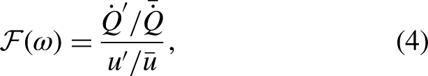
Assessing the thermoacoustic performance of designed combustors, with a focus on the stability quality factor, is crucial. Thermoacoustic instability in combustion appliances arises from intricate interactions among unsteady combustion, heat transfer, and (maybe) acoustic modes within the system. Accurate prediction of system stability requires modeling all components, including the burner with flame. Traditionally, the burner in the presence of combustion is represented as an acoustically (active) two-port block with passive upstream and downstream acoustic terminations. The dispersion relation of the thermoacoustic system is commonly used for anticipating eigen-frequencies and assessing stability. However, practical scenarios often lack specific information about upstream and downstream terminations during development. This raises a critical question: How can the thermoacoustic performance of burners and their associated flames be evaluated without specified acoustics? This article addresses this question by exploring the concept of unconditional stability in a generic two-port thermoacoustic system. The unconditional stability criteria have been used as quality indicators in designing electrical devices. This rich toolbox has been introduced in thermoacoustics. We first scrutinize assumptions underlying two most known unconditional stability-based criteria called $\mu$ and $k$ factors, connecting them to the general thermoacoustic problems. Then, the application of these criteria in assessing the thermoacoustic quality of burners with flames are discussed. This investigation revealed that while they are able to accurately predict the histogram of unstable frequencies and critical frequency bands, their use as reliable indicators to assess thermoacoustic quality in burners are not recommended due to their mathematical limitations and high level of conservatism of these factors.

Introduction

The requirement for reducing pollutants in combustion systems has driven the development of premixed combustion, which unfortunately is susceptible to thermoacoustic instabilities. To address this issue, one approach is to design an acoustically stable combustor^1–3 based on a given passive acoustic embedding.

However, during the development phase of a burner, information about the up/downstream acoustics of the specific industrial system in which the burner will be used is often unavailable. This lack of knowledge necessitates designing a burner, along with its corresponding flame, to operate stably across a wide range of possible up/downstream acoustic terminations. Evaluating and comparing thermoacoustic quality of burners with their corresponding flames, “figure-of-merit for thermoacoustic stability,” becomes crucial in achieving this goal.

Traditionally, the understanding of these instabilities has been influenced by the belief that the acoustic terminations and the burner with flame are closely interconnected. However, adopting a one-dimensional network modeling strategy can contribute to a better comprehension of the flame-acoustic coupling. ⁴ In this approach, the output of one element serves as the input for the next connected element, effectively representing a combustion system as a network.

Inspired by the concept of whistling potentiality for a generic two-port network introduced by Aurégan and Starobinski, ⁵ Gentemann and Polifke, ⁶ and Polifke ⁷ pioneered the concept of the figure-of-merit in thermoacoustics based on an activity/passivity check. The proposed formulations provide insights into the frequency range where the flame regardless of surrounding acoustic environment acts either as a source or a sink of acoustic energy. This concept could prove beneficial in optimizing a two-port (active) device to attain maximum amplification of acoustic power ⁸ . However, the exclusion of acoustic losses from the environmental representation has identified this criterion as ultra-conservative.^7,9 It consistently indicates a very narrow frequency range for the flame to be classified as a passive element. Moreover, there was no direct comparison among multiple burners with their flames to illustrate how one can compare the thermoacoustic quality of various burners with their corresponding flames.

In 2015, Kornilov and de Goey ¹⁰ explored the possibility of utilizing a Monte Carlo (MC) simulation to examine the stability of a burner with its corresponding flame embedded in a system equipped with randomly selected sets of frequency-independent upstream and downstream reflection coefficient values. They introduced a performance metric called the probability of instability, calculated by counting the number of unstable cases in the MC simulation divided by the total number of cases. Subsequently, Saxena et al.^11,12 extended this MC simulation using the concept of strictly positive real functions to generate a set of frequency-dependent reflection coefficients.

The two-port representation of constituent elements is commonly used to facilitate low-order network modeling in other research fields, for example, in designing electrical circuits. Various conservative criteria have been developed to predict the unconditional or conditional stability of networks. One widely employed method involves forming stability circles in the imaginary frequency domain by applying the concept of infinite phase margin to the open-loop systems. ¹³

Kornilov and de Goey ¹⁴ delved into the examination of the burner’s figure-of-merit ¹⁰ and investigated the potential application of microwave theory’s toolbox in thermoacoustic contexts. Their primary focus was on the concept of activity/passivity along with unconditional stability, where they integrated the flame transfer function (TF) into the Rankine-Hugoniot jump condition, treating the scattering matrix of the flame as the singular active two-port device. They introduced three key concepts in their research, which are elaborated upon in the subsequent discussion. The authors introduced two widely recognized and commonly employed criteria from the field of amplifier design to the realm of thermoacoustics called the Rollett factor $k$ and Edwards-Sinsky factor $\mu$ . Although the exact procedures and underlying assumptions for obtaining these criteria were not explicitly provided in this work, their results exhibited a promising correlation with the unstable frequency distribution obtained from MC simulations ¹⁰ . This suggests that the Rollett factor ( $k$ ) and Edwards-Sinsky factor ( $\mu$ ) may serve as effective tools in assessing thermoacoustic quality.

Building upon these findings, Kojourimanesh et al. ¹⁵ provided algebraic mathematical proofs for a deeper understanding of the concepts of unconditional and conditional stability within the framework of microwave theory. However, much like other studies in this domain, there has been a lack of direct comparisons between different burners and their corresponding flames to unveil the practical potential of these criteria in ranking various burners based on their thermoacoustic qualities. Consequently, the capacity of these factors to function as a “figure-of-merit in thermoacoustics” remains uncertain.

In contrast to previous studies,^14,15 which primarily focused on the applicability of the $\mu$ and $k$ factors as a figure-of-merit in thermoacoustics, our work aims to critically examine and challenge this idea. We here provide a comprehensive analysis of the limitations and potential pitfalls associated with using these criteria for direct comparison among different burners with flames. By addressing these critical aspects, our work seeks to contribute to a better understanding of the limitations of the Rollett conditions and the Edwards-Sinsky factor, and provide valuable insights for the development of more accurate and reliable figure-of-merit approaches for assessing thermoacoustic stability in burners with flames.

This article is structured as follows: In the “Methodology” section, we provide a brief overview of the main features of thermoacoustic systems based on a network modeling approach. We then discuss the relevant fundamental concepts of the argument principle to use as a starting point to delve into some assumptions in deriving these equations. The rest of the “Methodology” section is devoted to elaborating on the figure-of-merit based on the concept of unconditional stability, and the Rollett ( $k$ ) and Edwards-Sinsky ( $\mu$ ) factors. In the “Numerical example” section, by way of examples, we demonstrate how these factors may lead to incorrect evaluation of the thermoacoustic quality of burners with their corresponding flames. In the “Conclusion” section, after a brief recap of the main findings, we formulate our conclusions and perspectives.

Methodology

Network modeling and dispersion relation

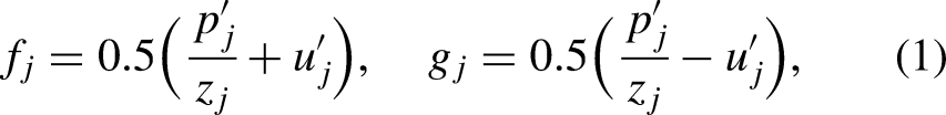
To apply one-dimensional linear acoustic network modeling in the frequency domain, the frequency range of interest should be smaller than the cut-off frequency of the first transverse mode ¹⁶ that is usually valid in thermoacoustics. There are several possibilities for the variables used to express the transfer matrices of the elements. Here let us focus on the Riemann invariants $f_j$ and $g_j$ where are written in terms of the complex acoustic pressure $p_j^{\prime }$ and the acoustic particle velocity $u_j^{\prime }$ . Where $j=1,2$ , and the numbers 1 and 2 indicate upstream and downstream, respectively. At the limit of zero Mach number, we have

$$f_j=0.5(\frac{p_j^{\prime }}{z_j}+u_j^{\prime }),g_j=0.5(\frac{p_j^{\prime }}{z_j}-u_j^{\prime })$$

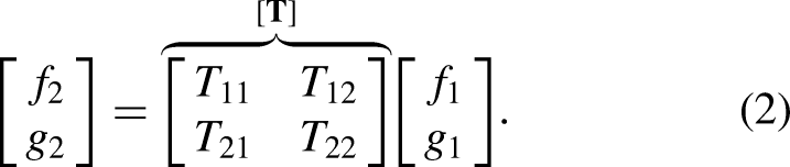
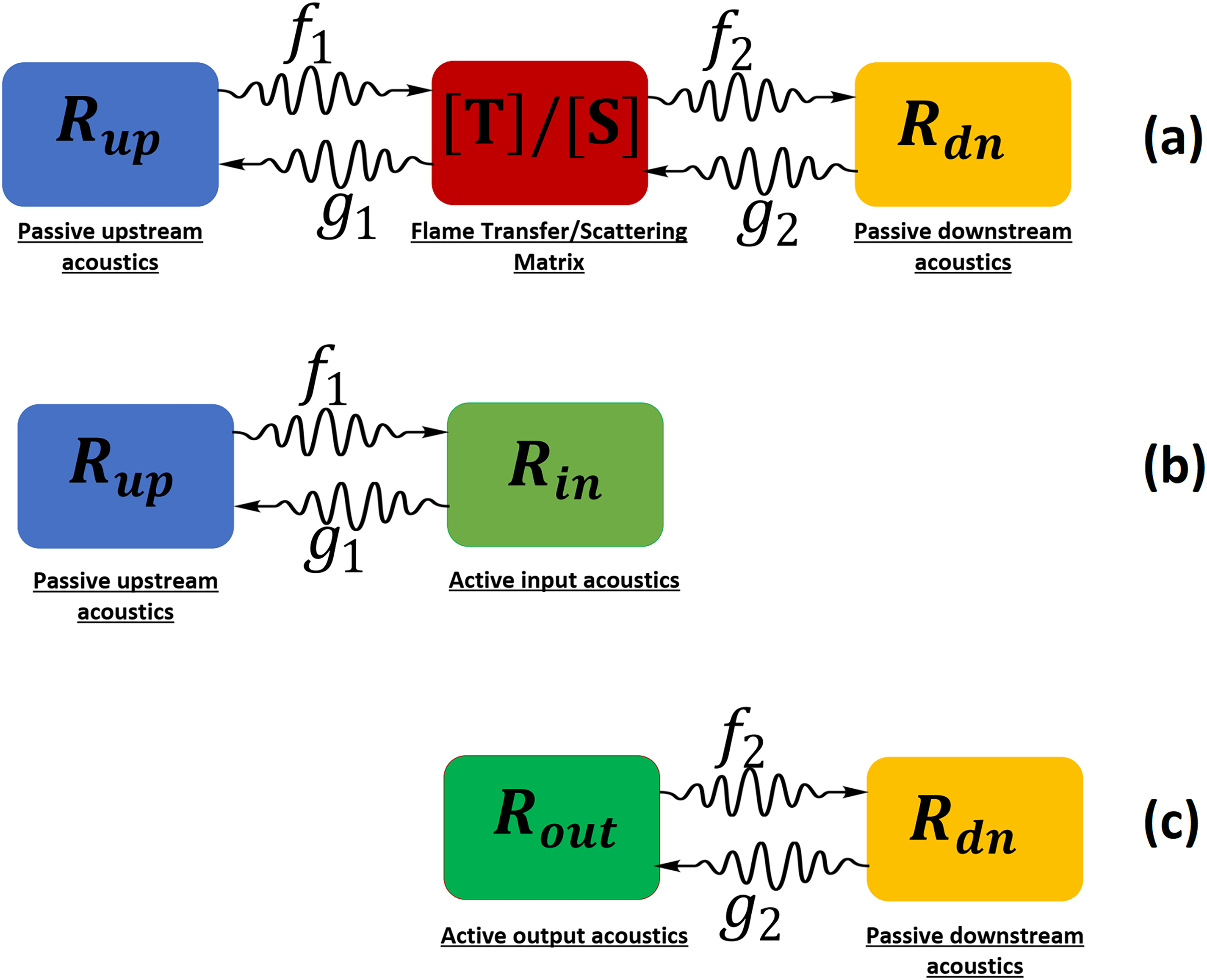
(1)where characteristic impedance can be defined as $z_j={\rho }_{0j}{c}_{0j}$ and ${\rho }_{0j}$ and $c_{0j}$ are, respectively, the densities and speed of sound in the fluid. ¹⁶ Note that values of ${\rho }_{0j}$ and $c_{0j}$ are different at up/down-stream of the burner. When the forward and backward travelling waves at one (physical) side of the element are written as a function of the ones at the other side (see Figure 1(a)), interrelations which involves a so-called the transfer matrix T is obtained as follows:

$$\left[\begin{array}{c}{f}_2\\ g_2\end{array}\right]=\stackrel{[\mathbf{T}]}{\overbrace{\left[\begin{array}{cc}{T}_{11}& T_{12}\\ T_{21}& T_{22}\end{array}\right]}}\left[\begin{array}{c}{f}_1\\ g_1\end{array}\right]$$

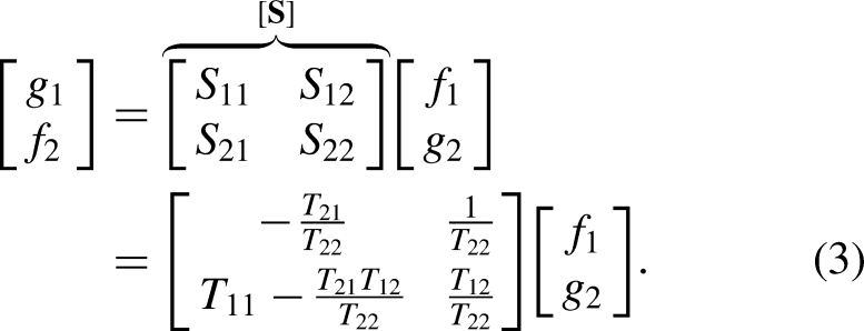
(2)One can arrive at a particularly insightful description if the equations of T are rearranged such that the ingoing waves $(f_1,g_2)$ appear as inputs to the matrix, and the outgoing waves $(g_1,f_2)$ as outputs. In that case, the so-called scattering matrix S is obtained. The diagonal elements $S_{11}$ and $S_{22}$ represent the reflection coefficients as seen from the up- and down-stream sides of the element, whereas $S_{21}$ and $S_{12}$ indicate the transmission coefficients to the up- and down-stream sides, respectively.

$$\left[\begin{array}{c}{g}_1\\ f_2\end{array}\right]=\stackrel{[\mathbf{S}]}{\overbrace{\left[\begin{array}{cc}{S}_{11}& S_{12}\\ S_{21}& S_{22}\end{array}\right]}}\left[\begin{array}{c}{f}_1\\ g_2\end{array}\right]=\left[\begin{array}{cc}-\frac{T_{21}}{T_{22}}& \frac{1}{T_{22}}\\ T_{11}-\frac{T_{21}{T}_{12}}{T_{22}}& \frac{T_{12}}{T_{22}}\end{array}\right]\left[\begin{array}{c}{f}_1\\ g_2\end{array}\right]$$

(3)

Figure 1.

Generic 1D acoustic network model of a combustion system; (a) MIMO layout; SISO representation, (b) in the input plane; and (c) in the output plane. MIMO: multiple-input-multiple-output; SISO: single-input-single-output; 1D: one-dimensional.

In thermoacoustics, the common situation is encountered when the heat release is concentrated in a region much smaller than the acoustic wavelength. Therefore, the conservation equations for the flame can be reduced to jump conditions known as Rankine-Hugoniot (R-H) relations. To obtain the relationship between the acoustic quantities up/down-stream of the flame, one needs a closure relationship. For laminar premixed flames, it is generally assumed that the heat release fluctuations are mainly due to the velocity fluctuations upstream of the flame. In this case, one can define a flame TF ( $\mathcal{F}(\omega )$ ) as the normalized ratio of the heat release rate fluctuation ${\dot{Q}}^{\prime }/\overline{\dot{Q}}$ to the normalized ration of acoustic velocity excitation $u^{\prime }/\overline{u}$ at some reference location upstream of the burner.

$$\mathcal{F}(\omega )=\frac{{\dot{Q}}^{\prime }/\overline{\dot{Q}}}{u^{\prime }/\overline{u}}$$

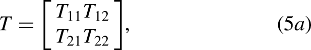
(4)where $\overline{\dot{Q}}$ , $\overline{u}$ are the mean heat release rate and unburned mixture velocity, respectively. By substituting $\mathcal{F}(\omega )$ into acoustic R-H relations, the flame transfer matrix according to equation (5a) to (5c) can be written as Manohar ¹⁷ :

$$T=\left[\begin{array}{c}{T}_{11}{T}_{12}\\ T_{21}{T}_{22}\end{array}\right]$$

(5a)

$$T_{11}=T_{22}=0.5(ϵ+1+\theta \mathcal{F})$$

(5b)

$$T_{12}=T_{21}=0.5(ϵ-1-\theta \mathcal{F})$$

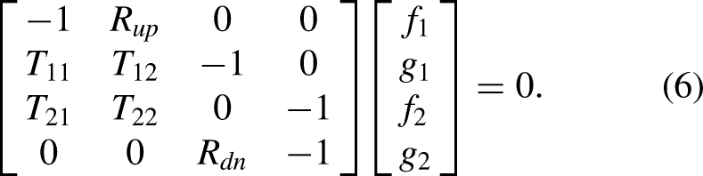
(5c)where $\theta =T_2/T_1-1$ is the temperature jump, $ϵ={\rho }_{01}{c}_{01}/{\rho }_{02}{c}_{02}$ the specific impedance jump across the flame. For the abstract model in terms of the scattering matrix $S$ , as shown in Figure 1(a)), the total set of system equations, is given by,

$$\left[\begin{array}{cccc}-1& R_{up}& 0& 0\\ T_{11}& T_{12}& -1& 0\\ T_{21}& T_{22}& 0& -1\\ 0& 0& R_{dn}& -1\end{array}\right]\left[\begin{array}{c}{f}_1\\ g_1\\ f_2\\ g_2\end{array}\right]=0$$

(6)Note that all entries of $T_{ij}$ , as well as the upstream and downstream reflection coefficients $R_{up}$ and $R_{dn}$ , may depend on the Laplace variable $s=i\omega +\sigma$ . This dependency arises from the time dependence in the governing equations, which take the form $e^{+st}$ . This homogeneous system of linear equations has a nontrivial solution if the determinant of the corresponding system matrix is zero. It can be explicitly written as

$${\mathrm{\Pi }}^T=T_{22}-T_{12}{R}_{dn}+T_{21}{R}_{up}-T_{11}{R}_{up}{R}_{dn}=0$$

(7)A common practice is to search for the roots of the dispersion relation, equation (7), to obtain a set of eigen-frequencies. The roots (zeros) of this equation which are belonging to the right-half plane (RHP) of $s$ -plane represent the unstable (exponentially growing in time) solutions. However, here we avoid doing that.

Stability analysis in frequency domain

As the localization of the roots (zeros) of dispersion relation in s-plane is crucial to resolve the dilemma of the system stability-instability, one can use the corresponding analysis methods developed in the complex function analysis theory to approach this issue. In this section, we will begin by offering an extensive introduction to fundamental principles originating from the complex function theory. Afterward, we will explore how these principles can be practically applied to analyze the challenge of stability and simplify the task of stabilizing flames.

Cauchy’s argument principle ¹⁸

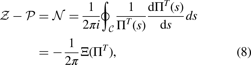
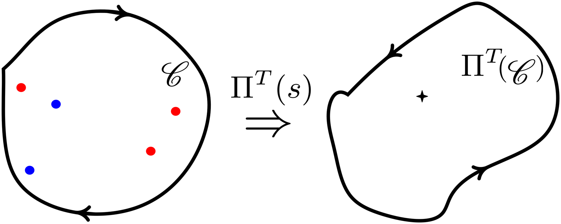
If ${\mathrm{\Pi }}^T(s)$ is a generic holomorphic function and nonzero at each point of a simple closed contour $\mathcal{C}$ and is meromorphic inside $\mathcal{C}$ , then

$$\mathcal{Z}-\mathcal{P}=\mathcal{N}=\frac{1}{2\pi i}{\oint }_{\mathcal{C}}\frac{1}{{\mathrm{\Pi }}^T(s)}\frac{\mathrm{d}{\mathrm{\Pi }}^T(s)}{\mathrm{d}s}ds=-\frac{1}{2\pi }\mathrm{\Xi }({\mathrm{\Pi }}^T)$$

(8)where $\mathcal{Z}$ and $\mathcal{P}$ are accordingly the number of zeros and poles of ${\mathrm{\Pi }}^T(s)$ evaluated in the domain encompassed by the contour $\mathcal{C}$ . $\mathcal{N}$ is known as the winding number of ${\mathrm{\Pi }}^T(\mathcal{C})$ , and counts the number of turns that the curve ${\mathrm{\Pi }}^T(\mathcal{C})$ winds clockwise around the origin. $\mathrm{\Xi }({\mathrm{\Pi }}^T)$ indicates the unwrapped argument of ${\mathrm{\Pi }}^T$ . Figure 2 shows a clarification example of Cauchy’s argument principle when ${\mathrm{\Pi }}^T$ is evaluated along contour $\mathcal{C}$ , in which blue and red circles represent zeros and poles of ${\mathrm{\Pi }}^T(s)$ , respectively. The number of encirclement can be easily calculated as $\mathcal{N}=2-3=-1$ .

Figure 2.

A clarification example of Cauchy’s argument principle. The blue and red circles represent zeros and poles of ${\mathrm{\Pi }}^T(s)$ in the $s$ -plane, respectively, and so the number of encirclements in ${\mathrm{\Pi }}^T(s)$ -plane around the origin shown with a black star can be calculated as $\mathcal{N}=2-3=-1$ .

Thermoacoustic stability analysis using Cauchy’s argument principle

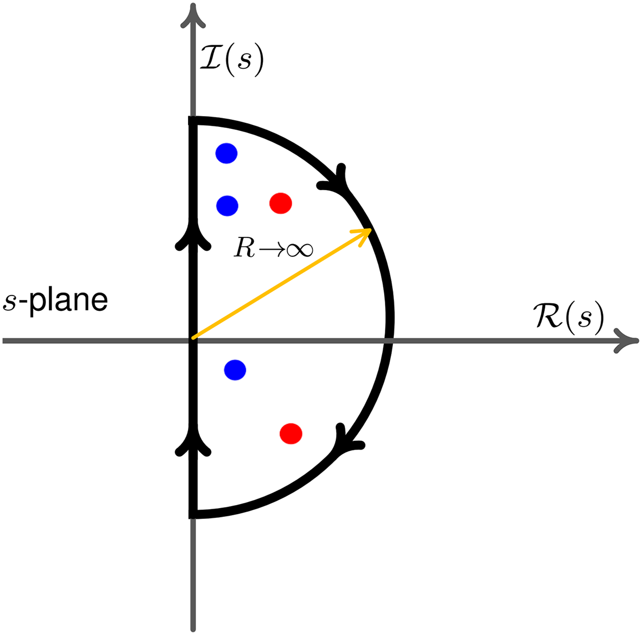
To assess the exponential stability of a linear thermoacoustic system, one must analyze the presence or absence of RHP zeros in the dispersion relation. The analysis based on the Cauchy’s argument principle enables the identification of RHP zeros and poles of the characteristic function ${\mathrm{\Pi }}^T(s)$ . To perform the corresponding evaluation, as depicted in Figure 3, Cauchy’s argument principle is applied by selecting the contour $\mathcal{C}$ to enclose the entire RHP ( $\mathcal{C}={\mathcal{D}}^{+}$ ). Accordingly, the function ${\mathrm{\Pi }}^T(s)$ must to be known along the imaginary axis and at infinity. In many physical systems, the frequency response ${\mathrm{\Pi }}^T(i\omega )$ is sufficient for assessing stability, especially when evaluating a (semi-)proper target function with the property $\underset{s\to +\mathrm{\infty }}{lim}{\mathrm{\Pi }}^T(s)=\text{constant}$ . In control theory, this approach is widely employed with the assistance of a graphical tool, namely the Nyquist plot. ¹⁹

Figure 3.

A clarification schematic of using Cauchy’s argument principle in right-half plane for stability analysis. The blue and red circles represent zeros and poles of ${\mathrm{\Pi }}^T(s)$ , respectively.

It is important to highlight that stability can also be determined by directly analyzing the argument of the dispersion relation. Recently, multiple thermoacoustic stability criteria based on different forms of the dispersion relation, along with their corresponding conservative forms, are established using the principle of argument. ²⁰ Before applying the argument principle in RHP of the complex domain, it is good to make two remarks:

Remark 1. For a passive single-input-single-output (SISO) system, the TF has no RHP poles. Since we are usually dealing with acoustically passive terminations, we can conclude that $R_{up}$ and $R_{dn}$ have no RHP poles.

Remark 2. Direct measurability of a SISO function is an indication of the absence of RHP poles. Therefore, the TF $\mathcal{F}$ and the coefficients of the transfer matrix $T_{ij}$ have no RHP poles.

Unconditional/inherent stability criteria for an active two-port device

In the design process of an active two-port device, achieving unconditional or inherent stability is a fundamental concept. It implies that the device will not oscillate under any combination of possible passive terminals. However, attaining unconditional stability in acoustics is a complex task. In this article, we aim to shed light on two widely used criteria for achieving unconditional stability: the Rollett conditions ( $k$ ) and the Edwards-Sinsky ( $\mu$ ) factor. Additionally, we will discuss the limitations associated with these requirements. Let us begin with the mathematical background of these requirements. Equation (7) represents the dispersion relation expressed in terms of a multiple-input-multiple-output (MIMO) representation. It can also be formulated as a SISO representation of the system, as depicted in Figure 1(b). In order to adopt the current approach, we reorganize the terms of the equation as follows. By dividing the dispersion equation (equation (7)) by $T_{22}-R_{dn}{T}_{12}$ , and using the transformation relation between transfer matrix and scattering matrix we obtain the following expression:

$${\mathrm{\Pi }}^T={\mathrm{\Pi }}_I^S\cdot \mathrm{den}[R_{in}^S]\cdot T_{22}=0$$

(9)where

$${\mathrm{\Pi }}_I^S=1-R_{up}{R}_{in}^S=0,R_{in}^S=S_{11}+\frac{S_{21}{S}_{12}{R}_{dn}}{1-S_{22}{R}_{dn}}$$

(10)where the operator $\mathrm{den}[\cdot ]$ indicates denominator of function $[\cdot ]$ , and variables ${\mathrm{\Pi }}_I^T$ and ${\mathrm{\Pi }}_I^S$ are named input dispersion relations based on the transfer matrix and scattering matrix, respectively. The terms $R_{in}^T$ and $R_{in}^S$ can be referred to as the input reflection coefficients based on the transfer matrix and scattering matrix, respectively, which are defined as $R_{in}^T=R_{in}^S=\frac{g_1}{f_1}$ (see Figure 1(b)). The SISO form of the dispersion equation is widely used in microwave theory,^13,21,22 and has already been applied to thermoacoustic problems.^23–26

Discussion I. From a broad perspective, the resemblance between microwave theory and thermoacoustics opens up possibilities for utilizing the extensive formalism of systems theory to establish a rigorous framework for studying thermoacoustic instabilities. However, there exists a fundamental difference in the approach employed by the two fields. In microwave theory, scattering matrices are directly measured, and as highlighted in Remark 2, it can be ensured that the scattering coefficients do not possess any RHP poles. In other words, according to the definition in equation (3), $T_{22}$ does not have any RHP zeros. Conversely, in thermoacoustics, the zeros of $T_{22}$ are referred to as intrinsic thermoacoustic (ITA) modes. Consequently, it can be concluded that the present notation is derived under the assumption of the absence of unstable intrinsic modes.

Input (plane) definitive stability (IDS) criterion based on ${\mathrm{\Pi }}^T={\mathrm{\Pi }}_I^S\cdot den[R_{in}^S]\cdot T_{22}=0$

²⁰

Using Cauchy’s argument principle in the RHP, we can rewrite equation (8) for the given dispersion relation in equation (9) as follows:

$${\mathcal{N}}_{{\mathrm{\Pi }}^T}={\mathcal{Z}}_{{\mathrm{\Pi }}^T}-{\mathcal{P}}_{{\mathrm{\Pi }}^T}$$

(11) ${\mathcal{Z}}_{{\mathrm{\Pi }}^T}$ and ${\mathcal{P}}_{{\mathrm{\Pi }}^T}$ can be written as follows:

$${\mathcal{Z}}_{{\mathrm{\Pi }}^T}={\mathcal{Z}}_{{\mathrm{\Pi }}_I^S}+{\mathcal{Z}}_{den[R_{in}^S]}+{\mathcal{Z}}_{T_{22}}$$

(12)

$${\mathcal{P}}_{{\mathrm{\Pi }}^T}={\mathcal{P}}_{{\mathrm{\Pi }}_I^S}+{\mathcal{P}}_{den[R_{in}^S]}+{\mathcal{P}}_{T_{22}}$$

(13)This means that to evaluate ${\mathrm{\Pi }}^T$ , one has to separately evaluate ${\mathrm{\Pi }}_I^S$ , $den[R_{in}^S]$ and $T_{22}$ . One can think of two scenarios here.

• First scenario: ${\mathcal{Z}}_{T_{22}}\ne 0$ and/or ${\mathcal{Z}}_{den[R_{in}^S]}\ne 0$ : This condition can be recognized as an artificial pole-zero cancellation case. A thermoacoustic system calls exponentially stable when ${\mathcal{Z}}_{{\mathrm{\Pi }}^T}=0$ . If one substitutes this requirement in equations (11) and (12):

  $${\mathcal{N}}_{{\mathrm{\Pi }}^T}=-{\mathcal{P}}_{{\mathrm{\Pi }}^T}$$
  (14)
  $${\mathcal{Z}}_{{\mathrm{\Pi }}_I^S}=-{\mathcal{Z}}_{den[R_{in}^S]}-{\mathcal{Z}}_{T_{22}}$$
  (15)The RHP poles of the $T_{22}$ is equal to RHP poles of the flame TF, so ${\mathcal{P}}_{T_{22}}={\mathcal{P}}_{\mathcal{F}}=0$ ; also with respect to the definition of $R_{in}^S$ , one can write ${\mathcal{P}}_{den[R_{in}^S]}={\mathcal{Z}}_{T_{22}}$ and ${\mathcal{P}}_{R_{in}^S}={\mathcal{Z}}_{den[R_{in}^S]}$ . Keeping in mind these equalities, after substituting equation (13) in equation (11):
  $${\mathcal{N}}_{{\mathrm{\Pi }}^T}=-{\mathcal{Z}}_{den[R_{in}^S]}-{\mathcal{Z}}_{T_{22}}$$
  (16)Equations (15) and (16) can be summarized as follows:
  $${\mathcal{N}}_{{\mathrm{\Pi }}^T}={\mathcal{Z}}_{{\mathrm{\Pi }}_I^S}$$
  (17)Equation (17) implies that even in cases of pole-zero cancellation with 100% fidelity, one still needs to evaluate the encirclement of the basic form of the dispersion relation given in equation (7) to provide information on the stability dilemma. Therefore, struggling with the dispersion relation in the form of the input plane as given in equations (9) and (10) is not useful. Another key conclusion is that the absence of RHP zeros of the input dispersion relation ( ${\mathcal{Z}}_{{\mathrm{\Pi }}_I^S}=0$ ) does not necessarily indicate anything regarding the stability dilemma. We will return to this point later in this article.

• Second scenario: ${\mathcal{Z}}_{T_{22}}=0$ and ${\mathcal{Z}}_{den[R_{in}^S]}=0$ : Using Cauchy’s argument principle in RHP, recalling equations (15) and (16) and substituting ${\mathcal{Z}}_{T_{22}}=0$ and ${\mathcal{Z}}_{den[R_{in}^S]}=0$ , the necessary and sufficient conditions for MIMO stability is the absence of encirclement for functions ${\mathrm{\Pi }}_I^S$ and $den[R_{in}^S]$ and it can be summarizes as follows:

  $${\mathcal{N}}_{{\mathrm{\Pi }}_I^S}={\mathcal{N}}_{den[R_{in}^S]}={\mathcal{N}}_{T_{22}}=0$$
  (18)In microwave theory ${\mathcal{N}}_{T_{22}}$ equals to zero due to the direct measurement of the scattering matrix. In the thermoacousics, in the case of direct assessment of scattering matrix (not flame TF) can be the case.

Input (plane) conservative stability (ICS) utilizing the concept of infinite phase margin ¹³

In the previous subsection, we derived sufficient conditions (though not necessary) to ensure the stability of a generic active two-port device in the absence of an unstable intrinsic mode, as described in equation (18). Now, the objective is here to establish a conservative stability criterion based on the concept of infinite phase margin. A system is said to have infinite phase margin if the magnitude of its open-loop SISO TF is always less than or equal to unity. In accordance with equation (18), we need to apply this concept to two components: the denominator of the input reflection coefficient ( $\text{den}[R_{in}^S]=1-{\mathcal{L}}_1$ , where ${\mathcal{L}}_1=S_{22}{R}_{dn}$ ) and the input dispersion relation ( ${\mathrm{\Pi }}_I^S=1-{\mathcal{L}}_2$ , where ${\mathcal{L}}_2=R_{up}{R}_{in}^S$ ):

$$|{\mathcal{L}}_1|<1\Rightarrow |S_{22}|<\frac{1}{|R_{dn}|}$$

(19)

$$|{\mathcal{L}}_2|<1\Rightarrow |R_{in}^S{R}_{up}|<1$$

(20)Starting from equation (20) and substituting equation (10), we can rewrite it as follows:

$$\begin{array}{rl}|R_{in}^S{R}_{up}|& =|S_{11}{R}_{up}+\frac{S_{21}{S}_{12}{R}_{up}{R}_{dn}}{1-S_{22}{R}_{dn}}|\\ & =\frac{|S_{11}^{\prime }-{\mathrm{\Delta }}^{\prime }{R}_{dn}|}{|1-S_{22}{R}_{dn}|}<1\end{array}$$

(21)where

$$S_{11}^{\prime }=S_{11}{R}_{up},S_{21}^{\prime }=S_{21}{R}_{up}$$

(22a)

$$\mathrm{\Delta }=S_{11}{S}_{22}-S_{12}{S}_{21},{\mathrm{\Delta }}^{\prime }=\mathrm{\Delta }{R}_{up}$$

(22b)If we set $|R_{in}{R}_{up}|=1$ , we establish a boundary of $R_{dn}$ in the input plane that separates stable from unstable regions:

$$|S_{11}^{\prime }-{\mathrm{\Delta }}^{\prime }{R}_{dn}|=|1-S_{22}{R}_{dn}|$$

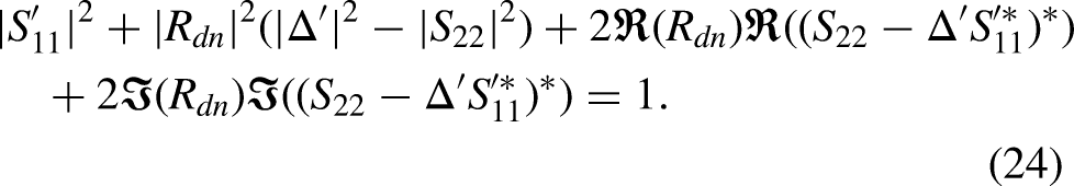
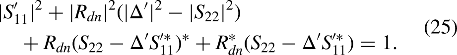
(23)We now proceed by squaring both sides of equation (23) and collecting terms, resulting in

$$\begin{array}{rl}& |S_{11}^{\prime }{|}^2+|R_{dn}{|}^2(|{\mathrm{\Delta }}^{\prime }{|}^2-|S_{22}{|}^2)+2\mathrm{\Re }(R_{dn})\mathrm{\Re }((S_{22}-{\mathrm{\Delta }}^{\prime }{S}_{11}^{\prime }*)*)\\ & +2\mathrm{\Im }(R_{dn})\mathrm{\Im }((S_{22}-{\mathrm{\Delta }}^{\prime }{S}_{11}^{\prime }*)*)=1\end{array}$$

(24)Which simplifies to:

$$\begin{array}{rl}& |S_{11}^{\prime }{|}^2+|R_{dn}{|}^2(|{\mathrm{\Delta }}^{\prime }{|}^2-|S_{22}{|}^2)\\ & +R_{dn}(S_{22}-{\mathrm{\Delta }}^{\prime }{S}_{11}^{\prime }*)*+R_{dn}*(S_{22}-{\mathrm{\Delta }}^{\prime }{S}_{11}^{\prime }*)=1\end{array}$$

(25)Adding $|S_{22}-{\mathrm{\Delta }}^{\prime }{S}_{11}^{\prime }*{|}^2/(|S_{22}{|}^2-|\mathrm{\Delta }{|}^2{)}^2$ to both sides of equation (25) results in

$$\begin{array}{rl}& |R_{dn}{|}^2+\frac{|S_{22}-{\mathrm{\Delta }}^{\prime }{S}_{11}^{\prime }*{|}^2}{(|S_{22}{|}^2-|{\mathrm{\Delta }}^{\prime }{|}^2{)}^2}-R_{dn}\frac{(S_{22}-{\mathrm{\Delta }}^{\prime }{S}_{11}^{\prime }*)*}{(|S_{22}{|}^2-|{\mathrm{\Delta }}^{\prime }{|}^2{)}^2}\\ & -R_{dn}*\frac{(S_{22}-{\mathrm{\Delta }}^{\prime }{S}_{11}^{\prime }*)}{(|S_{22}{|}^2-|{\mathrm{\Delta }}^{\prime }{|}^2{)}^2}\\ & =\frac{(|S_{11}^{\prime }{|}^2-1)(|S_{22}{|}^2-|{\mathrm{\Delta }}^{\prime }{|}^2{)}^2+|S_{22}-{\mathrm{\Delta }}^{\prime }{S}_{11}^{\prime }*{|}^2}{(|S_{22}{|}^2-|{\mathrm{\Delta }}^{\prime }{|}^2{)}^2}\end{array}$$

(26)Equation (25) is of the form of a circle in the input plane for $R_{dn}$ , that is

$$|R_{dn}-C_i{|}^2=|R_i{|}^2$$

(27a)where

$$C_i=\frac{(S_{22}-{\mathrm{\Delta }}^{\prime }{S}_{11}^{\prime }*)*}{|S_{22}{|}^2-|{\mathrm{\Delta }}^{\prime }{|}^2},R_i=\frac{|S_{21}^{\prime }{S}_{12}|}{|S_{22}{|}^2-|{\mathrm{\Delta }}^{\prime }{|}^2}$$

(27b)are the center and radius of this circle, respectively. The stability circles represent the boundaries of permitted terminations in their respective reflection coefficient planes. To find whether the interior or exterior of the stability circles is representing the stable region, we set $R_{dn}=0$ , which results in $|R_{up}{R}_{in}|=|S_{11}^{\prime }|$ . So, we can, therefore, say that, if $|S_{11}^{\prime }|<1$ , the origin of the downstream plane in the Smith chart (unit circle) must lie in the stable region. Stability circles are a visualization tool for analyzing the stability of a system using the complex unit circle. In microwave theory, the goal is to find a suitable set of up/down-stream termination. The stability circles represent the boundaries of permitted terminations in their respective reflection coefficient planes. Since unconditional stability means that there are no possibilities that a passive termination trigger instabilities, a number of researchers worked to obtain a quality factor to check whether an amplifier is unconditionally stable.^27–31,21 It will be discussed in the following subsections.

Edwards-Sinsky ( $\mu$ ) criterion

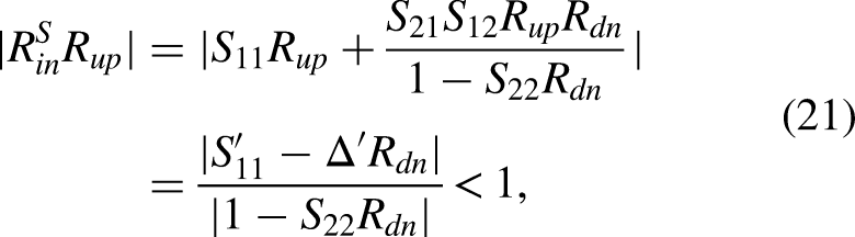
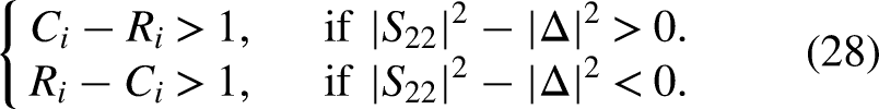
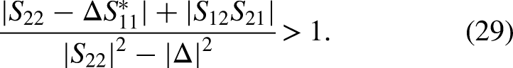
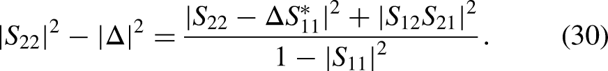
Taking into consideration the prerequisites for unconditional stability, Edwards and Sinsky ²⁸ considered a highly unfavorable scenario where $|R_{up}|=|R_{dn}|=1$ . By deriving the expression for stability circles, they were able to establish the conditions necessary for an unstable region to exist outside the downstream unit circle.

$$\{\begin{array}{cc}{C}_i-R_i>1,& \text{if }|S_{22}{|}^2-|\mathrm{\Delta }{|}^2>0\\ R_i-C_i>1,& \text{if }|S_{22}{|}^2-|\mathrm{\Delta }{|}^2<0\end{array}$$

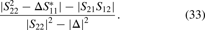
(28)Using algebraic work to quantify the minimum distance from the center of the unit circle to the unstable region, in both cases one arrives the similar relation as follows:

$$\frac{|S_{22}-\mathrm{\Delta }{S}_{11}*|+|S_{12}{S}_{21}|}{|S_{22}{|}^2-|\mathrm{\Delta }{|}^2}>1$$

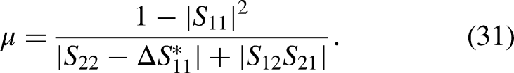
(29)The denominator of equation (29) can be eliminated and the expression can be further simplified by noting that Edwards and Sinsky: ²⁸

$$|S_{22}{|}^2-|\mathrm{\Delta }{|}^2=\frac{|S_{22}-\mathrm{\Delta }{S}_{11}*{|}^2+|S_{12}{S}_{21}{|}^2}{1-|S_{11}{|}^2}$$

(30)Finally, by introducing equation (30) in equation (29) a criterion known as the $\mu$ factor can be drived. This factor serves as a measure of the required margin of stability:

$$\mu =\frac{1-|S_{11}{|}^2}{|S_{22}-\mathrm{\Delta }{S}_{11}*|+|S_{12}{S}_{21}|}$$

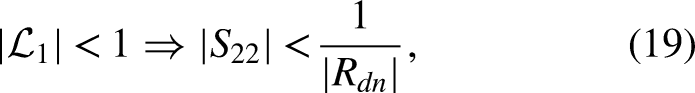
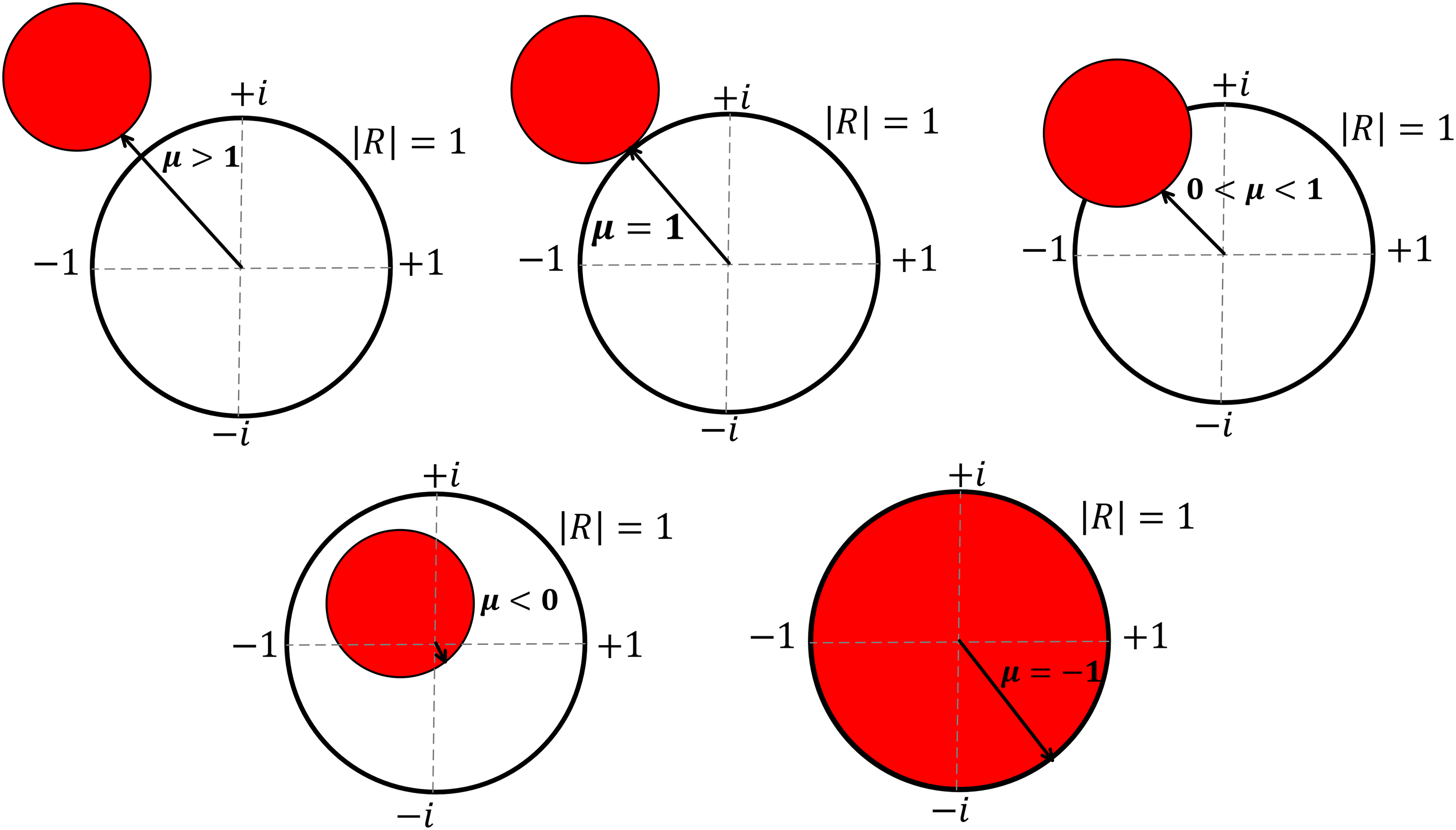
(31)In Figure 4, we have depicted several scenarios for better visual understanding. It should be noted that $\mu$ usually has different values in a frequency range and this should be independently interpreted. The red circles schematically illustrate the stability circle, while the white circle with a radius of unity represents the complex unit circle encompassing all possible values of reflection coefficients for a passive termination. Referring to Figure 4, if the $\mu$ factor is greater than or equal to 1 across the entire frequency range, a generic target device (in this case, a burner with a flame) is deemed unconditionally stable. This implies that the system will remain stable irrespective of the upstream and downstream terminations. When the $\mu$ factor is less than unity but still positive (i.e. $0<\mu <1$ ), even if it’s limited to a narrow frequency range, the center of the unit circle denotes the region of termination that ensures stability. In this case, the system is considered conditionally stable, as it necessitates specific termination conditions within that frequency range to maintain stability. In the scenario where $-1<\mu <0$ , the center of the complex unit circle represents the unsafe region corresponding to the termination at that specific frequency. Lastly, when $\mu =-1$ or $\mu <-1$ , the unsafe region encompasses the entire area of the complex unit circle even at single frequency, indicating that it is not possible to consider this system conditionally stable with infinite phase margin under.

Figure 4.

Schematic diagram indication of unsafe regions (red circle) and their relation with the $\mu$ factor in the complex unit circle (white circle).

Edwards and Sinsky proved that in the case of unconditional stability, that is, $\mu >1$ , $|S_{22}|$ should be smaller than unity. Therefore, for unconditional stability there is no need to evaluate directly $|S_{22}|<1$ according to equation (19).

Rollett ( $k$ ) factor

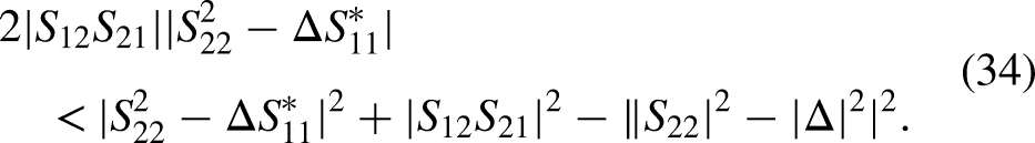
To obtain the Rollett factor one can follow a similar procedure to form the $\mu$ factor, but this time starting from

$$R_i-|C_i|>1$$

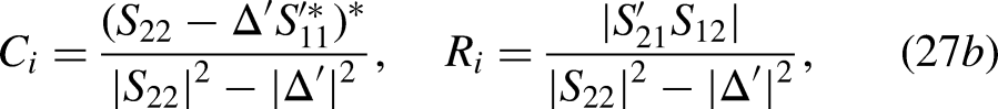
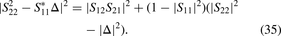
(32)Substituting equation (27a) and (27b) into equation (32) results in

$$\frac{|S_{22}^2-\mathrm{\Delta }{S}_{11}*|-|S_{21}{S}_{12}|}{|S_{22}{|}^2-|\mathrm{\Delta }{|}^2}$$

(33)Rearranging equation (33) and squaring both sides

$$\begin{array}{rl}& 2|S_{12}{S}_{21}||S_{22}^2-\mathrm{\Delta }{S}_{11}*|\\ & <|S_{22}^2-\mathrm{\Delta }{S}_{11}*{|}^2+|S_{12}{S}_{21}{|}^2-\Vert S_{22}{|}^2-|\mathrm{\Delta }{|}^2{|}^2\end{array}$$

(34)Note that the term $|S_{22}^2-S_{11}*\mathrm{\Delta }{|}^2$ can be expressed as follows:

$$|S_{22}^2-S_{11}*\mathrm{\Delta }{|}^2=|S_{12}{S}_{21}{|}^2+(1-|S_{11}{|}^2)(|S_{22}{|}^2-|\mathrm{\Delta }{|}^2)$$

(35)Substituting equation (35) into equation (34) yields

$$2|S_{12}{S}_{21}|<1-|S_{11}{|}^2-|S_{22}{|}^2+|\mathrm{\Delta }{|}^2$$

(36)This leads to the definition of the Rollett stability factor as follows:

$$k=\frac{1-|S_{11}{|}^2-|S_{22}{|}^2+|\mathrm{\Delta }{|}^2}{2|S_{12}{S}_{21}|}$$

(37)and the Rollett criterion to ensure unconditional stability as follows:

$$k>1.$$

(38)Discussion II. The $\mu$ and $k$ criteria are derived based on the second scenario and the conditions described in equation (18). Hence, these formulations cannot be directly applied in the presence of an unstable ITA mode. It is important to note that the $\mu$ criterion solely represents the minimum distance between the unsafe zones of the upstream or downstream unit circle of reflection coefficients and the center of the unit circle. When $\mu >1$ , it indicates unconditional stability that the entire unit circle is within the safe region. In the next section, we demonstrate that it is generally not feasible to meet this requirement across the entire frequency range in thermoacoustic applications. When $-1<\mu <1$ , this criterion does not provide any information about the size of the safe area inside the unit circle. Additionally, both $\mu$ and $\kappa$ are derived under the assumption of fully reflective acoustic boundaries ( $|R_{up}|=|R_{dn}|=1$ ). In control theory, this assumption implies that the thermoacoustic system operates with infinite phase margin and under the most critical conditions for the gain margin.

Numerical example

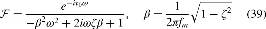
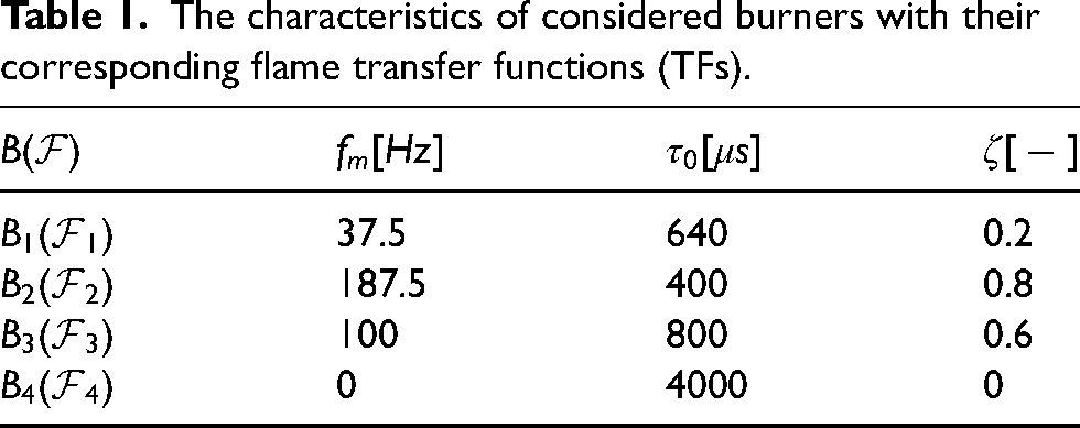
In order to demonstrate the limitations of these criteria, we will provide numerical examples in the absence of unstable ITA modes. We focus on this specific type of thermoacoustic system because we have already discussed its limitations in the presence of unstable ITA modes. Our objective is to show that these criteria cannot be used as a reliable figure-of-merit even in the absence of unstable ITA modes. To apply the concept introduced in the previous section, we need to consider different flame TFs and compare them to rank them based on their thermoacoustic stability quality. It is widely recognized that the thermoacoustic behavior of various practical flames can be approximated by a time-delayed second-order oscillation with a damping factor ( $\zeta$ ) as described by Hoeijmakers et al. ¹⁸ :

$$\mathcal{F}=\frac{e^{-i{\tau }_0\omega }}{-{\beta }^2{\omega }^2+2i\omega \zeta \beta +1},\beta =\frac{1}{2\pi f_m}\sqrt{1-{\zeta }^2}$$

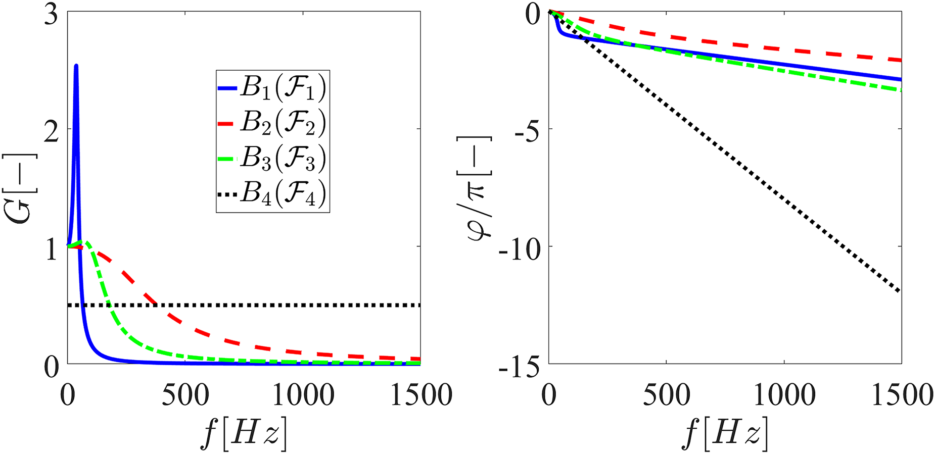
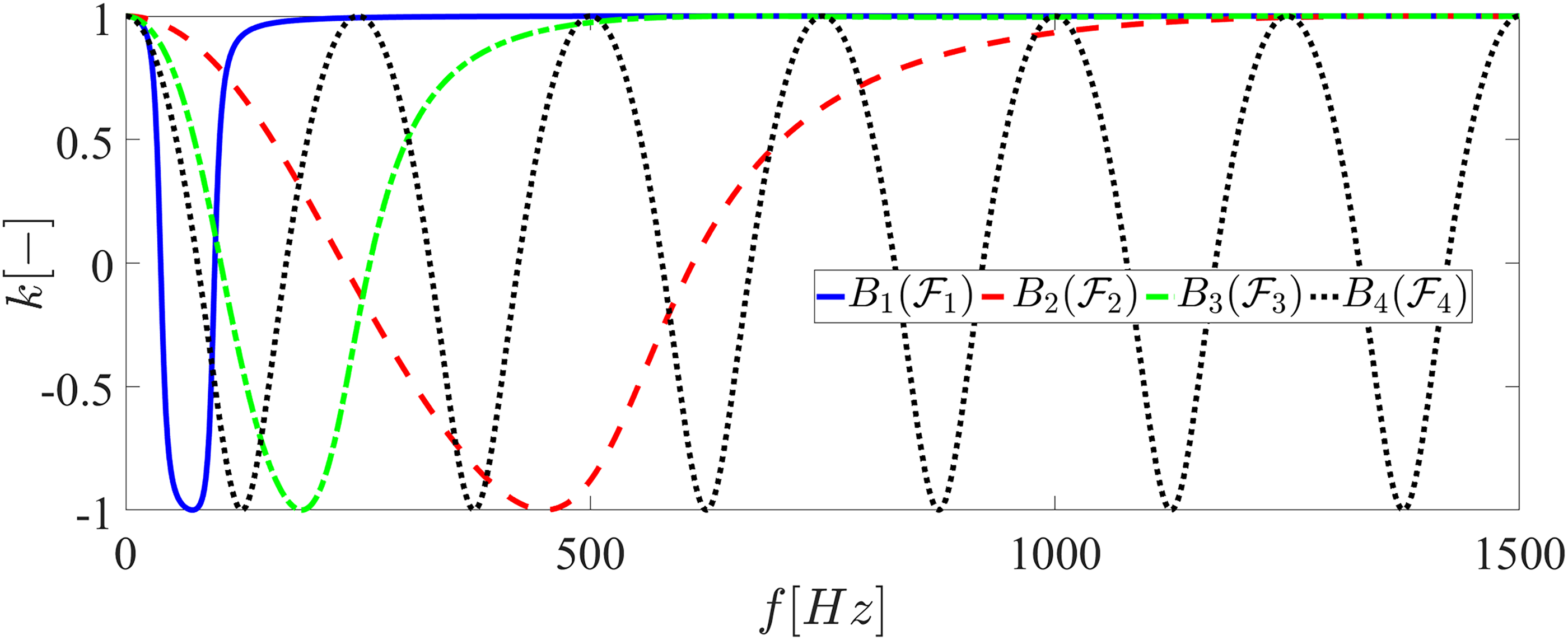
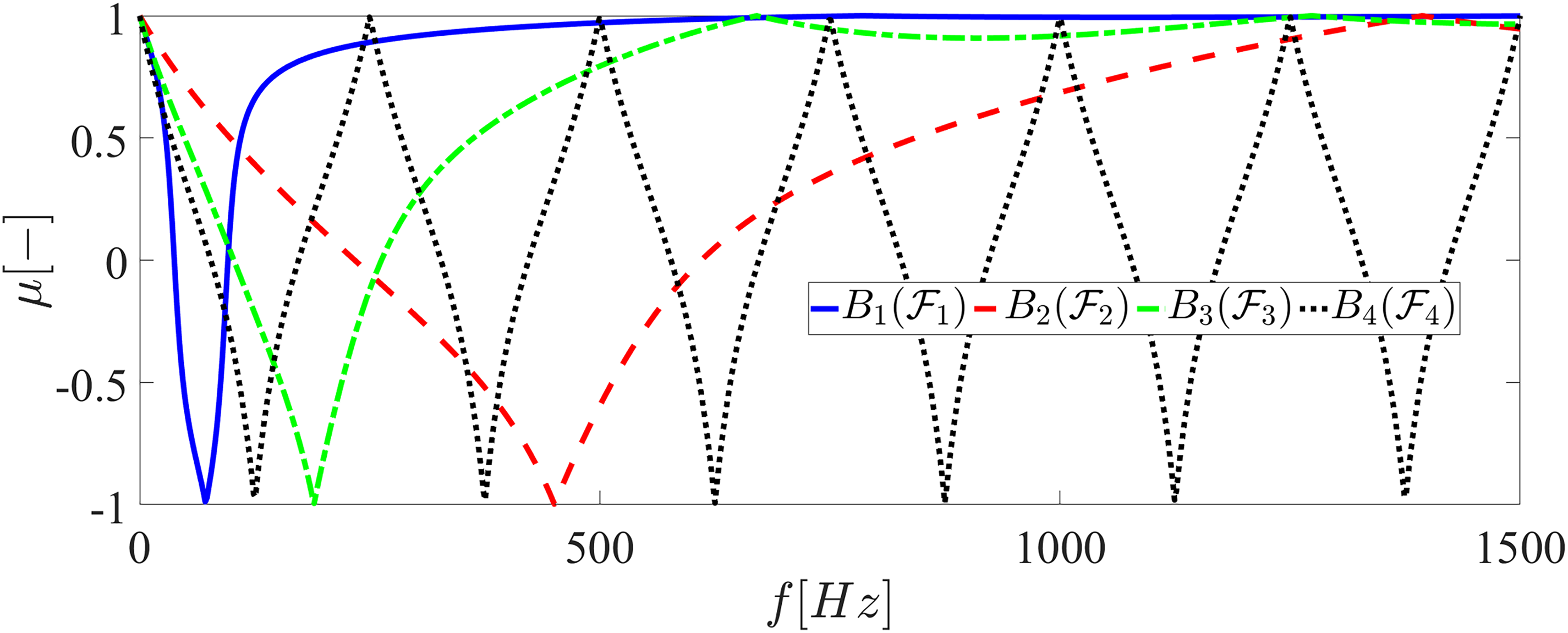
(39)where $\zeta$ and ${\tau }_0$ are the damping factor and the time delay, respectively. The $\omega =2\pi f$ is the angular frequency. $f$ and $f_m$ indicate the frequency and corresponding overshoot frequency. In the present work, Figure 5 shows four flame TFs, as given in Table 1

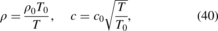
To form the transfer matrix, knowledge of upstream and downstream temperatures is required. Therefore, a fixed value of $T_1=300\text{K}$ is assumed, and a uniform temperature of $T_2=1900\text{K}$ representative of a realistic burner configuration is chosen for the downstream duct. Density and sound velocity can be defined as a function of temperature:

$$\rho =\frac{{\rho }_0{T}_0}{T},c=c_0\sqrt{\frac{T}{T_0}}$$

(40)where ${\rho }_0=1.29{\text{kg/m}}^3$ , $T_0=273\text{K}$ , and $c_0=331\text{m/s}$ . Now all the necessary components and terms have been introduced, we will examine if it is possible to compare different burners with their associated flames on the basis of the $\mu$ and $k$ criteria.

Figure 5.

The gain (right) and phase (left) of different flame transfer functions (TFs) according to Table 1.

Table 1.

The characteristics of considered burners with their corresponding flame transfer functions (TFs).

$B(\mathcal{F})$	$f_m[\mathit{\text{Hz}}]$	${\tau }_0[\mu \mathit{\text{s}}]$	$\zeta [-]$
$B_1({\mathcal{F}}_1)$	37.5	640	0.2
$B_2({\mathcal{F}}_2)$	187.5	400	0.8
$B_3({\mathcal{F}}_3)$	100	800	0.6
$B_4({\mathcal{F}}_4)$	0	4000	0

Insight into the $\mu$ and $k$ criteria

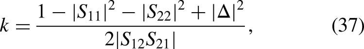
To obtain the scattering matrices of the burners with flames, one can substitute the flame TFs provided in Table 1 into equation (5a) to (5c) and then equation (3). By substituting the entries of the scattering matrix into equations (31) and (37), respectively, the variables $\mu$ and $k$ can be easily calculated. Figures 6 and 7 depict the variations of $k$ and $\mu$ with frequency, respectively. As expected, these variables exhibit similar qualitative and quantitative behavior. This alignment was anticipated since we demonstrated in the previous section that $k$ can be derived from $\mu$ through algebraic manipulation. Another important observation is that both variables vary between $-1$ and $1$ , which may be attributed to the symmetry of the transfer matrix in the vicinity of zero Mach number. Furthermore, this figure clearly demonstrates that neither $\mu$ nor $k$ can satisfy the requirement for unconditional stability, which necessitates values greater than unity for both variables in the entire frequency range.

Figure 6.

The Rollett factor $k$ versus the frequency. The information on different flame transfer functions (TFs) are given in Table 1.

Figure 7.

The Edwards-Sinsky factor $\mu$ versus the frequency. The information on different flame transfer functions (TFs) are given in Table 1.

As mentioned earlier, $\mu$ represents the minimum distance from the origin to the unsafe region inside the unit circle. This feature of $\mu$ provides an advantage compared to $\kappa$ . Although $\mu$ does not directly quantify the size of the unsafe region, a previous study by Kojourimanesh et al. ¹⁵ demonstrated that the size of the unsafe area inside the unit circle varies monotonically with $\mu$ . This relationship can be utilized in the analysis. Therefore, even though $\mu$ does not directly provide information about the size of the unsafe region, it can still effectively assess stability and enable relevant conclusions in the analysis, considering its monotonic relationship with the size of the unsafe area inside the unit circle. This distinction is important to make. Instead of using the term “unstable,” it is more accurate to refer to the regions as “unsafe” because the criteria are derived based on the concept of infinite phase margin and unconditional stability of subsystem.

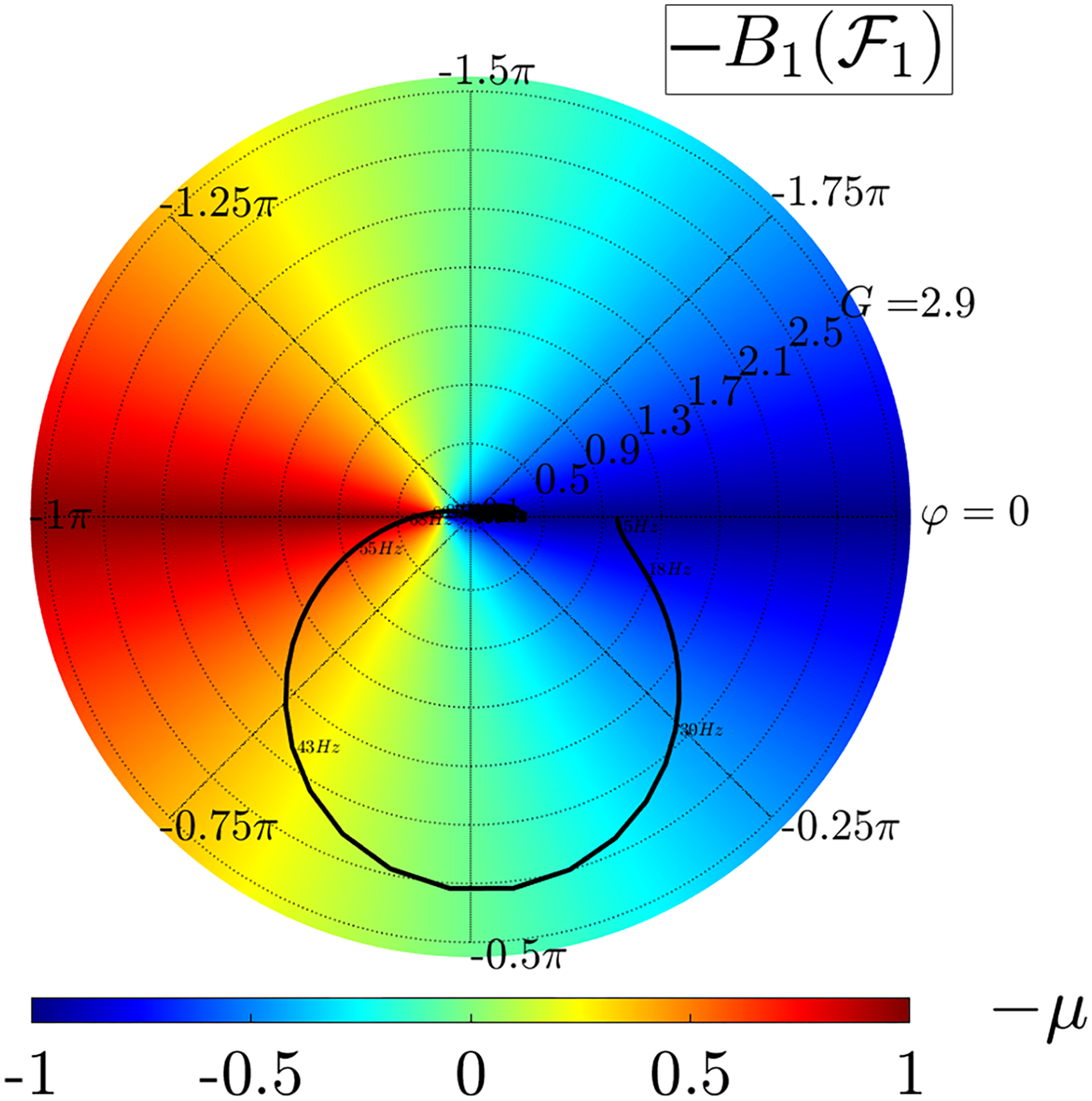
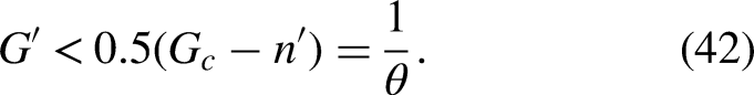
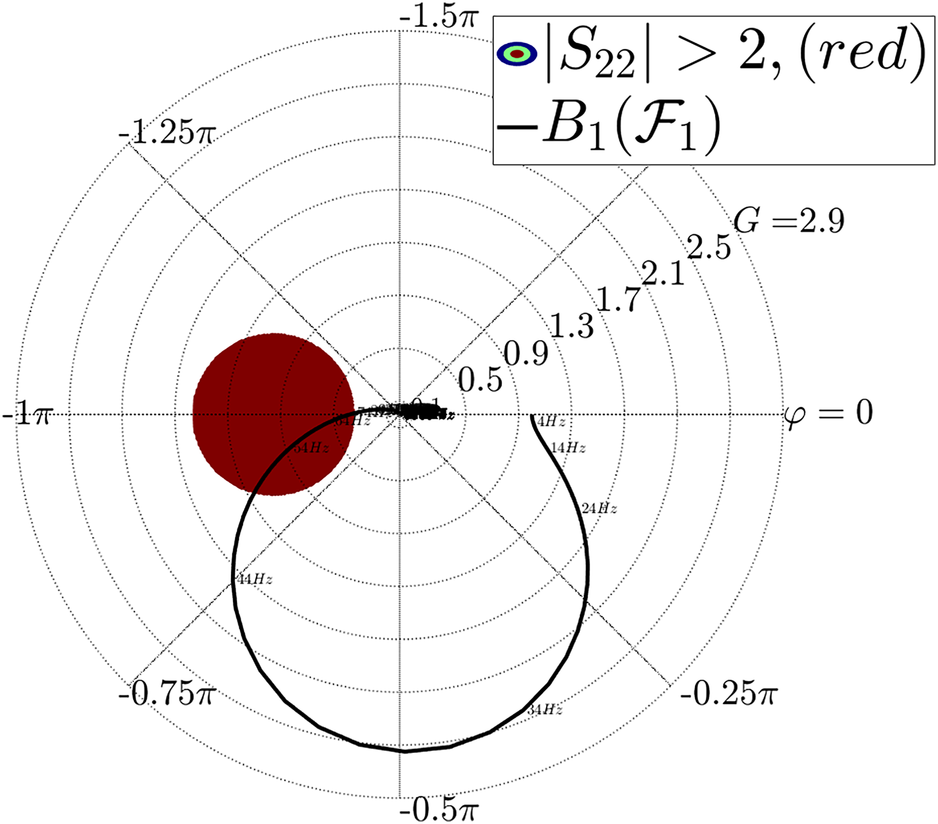
An insightful visual representation of the situation in hand can be obtained if to notice that $\mu$ can be treated as a real-valued function of complex valued variable, namely of the flame TF. Accordingly, it can be directly visualized using, for example, a contour plots. Figure 8 provides a comprehensive representation of the $\mu$ variable by evaluating it over a wide range of generic flame TFs $\mathcal{F}=G{e}^{i\phi }$ . The contour plot illustrates the variations of $\mu$ , while the dotted circles within the contour represent iso-flame-TF-gain, and the dotted straight lines represent iso-flame-TF-phase. As an example, the specific flame TF ${\mathcal{F}}_1$ is shown by a solid black curve within this plot. To highlight better the more critical region, we have plotted $-\mu$ , showing negative $\mu$ values in red, on this graph. It can be observed that when the phase of the flame TF crosses $-\pi$ , it corresponds to the most critical region based on this criterion. This observation aligns well with the concept of an ITA mode. However, it appears to be more conservative than the requirements for the ITA mode, and can be demonstrated through algebraic analysis.

Figure 8.

The contour plot of the $-\mu$ factor in by considering arbitrary values for flame transfer function (TF).

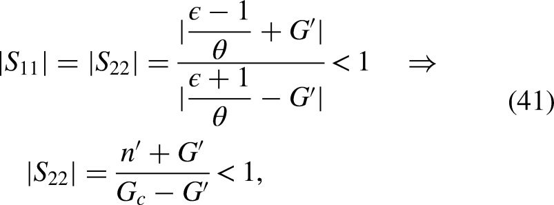
From the concept of ITA in the vicinity of zero Mach number, ³² where $T_{22}=0$ , it is known that the pure ITA mode is unstable when the gain of the flame TF is larger than the critical value ( $G\ge G_c=\frac{ϵ+1}{\theta }$ ) at frequencies where the phase crosses $-\pi \pm 2m\pi$ , with $m$ being an arbitrary positive integer. Based on equations (19) and (20), we can summarize the necessary requirement for $\mu >0$ and the necessary but not sufficient requirement for $\mu >1$ as $|S_{11}|=|S_{22}|<1$ . By substituting $\mathcal{F}=G{e}^{i\phi }$ into $T_{21}=0.5(ϵ-1-\theta \mathcal{F})$ and $T_{22}=0.5(ϵ+1+\theta \mathcal{F})$ , and considering the phase of the flame TF $\mathcal{F}$ crossing $-\pi \pm 2m\pi$ with $m$ being any positive integer, we can express the conditions as follows:

$$|S_{11}|=|S_{22}|=\frac{|\frac{ϵ-1}{\theta }+G^{\prime }|}{|\frac{ϵ+1}{\theta }-G^{\prime }|}<1\Rightarrow |S_{22}|=\frac{n^{\prime }+G^{\prime }}{G_c-G^{\prime }}<1$$

(41)where $G^{\prime }$ indicates the gain of $\mathcal{F}$ at the frequency where it phase crossing $-\pi \pm 2m\pi$ , and clearly $n^{\prime }$ is always smaller than $G_c$ . Now it can be argued:

$$G^{\prime }<0.5(G_c-n^{\prime })=\frac{1}{\theta }$$

(42)Equation (42) clearly shows that $G^{\prime }<G_c$ . It means that the requirement for $\mu >0$ is stricter than the requirement for the instability of the ITA mode.

For further clarification, a contour plot of the argument of $T_{22}$ and a contour plot of the module of $S_{22}$ are presented in Figures 9 and 10, respectively. In Figure 9, the concept of ITA mode can be interpreted. The $\pi$ -wrapped argument of $T_{22}$ is shown, and a phase jump transition is observed when the phase of the TF crosses $-\pi$ and the gain of the flame TF exceeds a critical value ( $G_{cr}$ ) slightly < $0.7$ . Through calculations, it has been determined that this critical gain represents the threshold for the stable ITA mode. According to the requirements for the unstable ITA mode, a phase crossing of $-\pi$ should occur along with a gain greater than $G_{cr}$ . This graph clearly shows that the blue-to-red transition (phase jump) only happens for gains greater than $G_{cr}$ . The white region within the contour plot corresponds to the argument of $T_{22}$ in the vicinity of $0$ , and it occurs when the phase of the flame TF crosses $2m\pi$ , where $m$ can be any positive integer, with no restrictions on the gain.

Figure 9.

Contour plot of the argument of transfer matrix coefficient $T_{22}$ . The critical gain $G_{cr}$ is shown with a black diamond.

Figure 10.

Evaluation of the scattering matrix coefficient $|R_{dn}\Vert S_{22}|$ with $|R_{dn}|=1$ .

This visual representation highlights that for the ITA mode, if the flame TF crosses the negative real axis in the polar plot with a sufficiently large gain ( $G>G_{cr}$ , which is necessary and sufficient for the occurrence of encirclement according to winding number), the ITA mode is present. Hence, we have visually demonstrated the ITA mode through this representation.

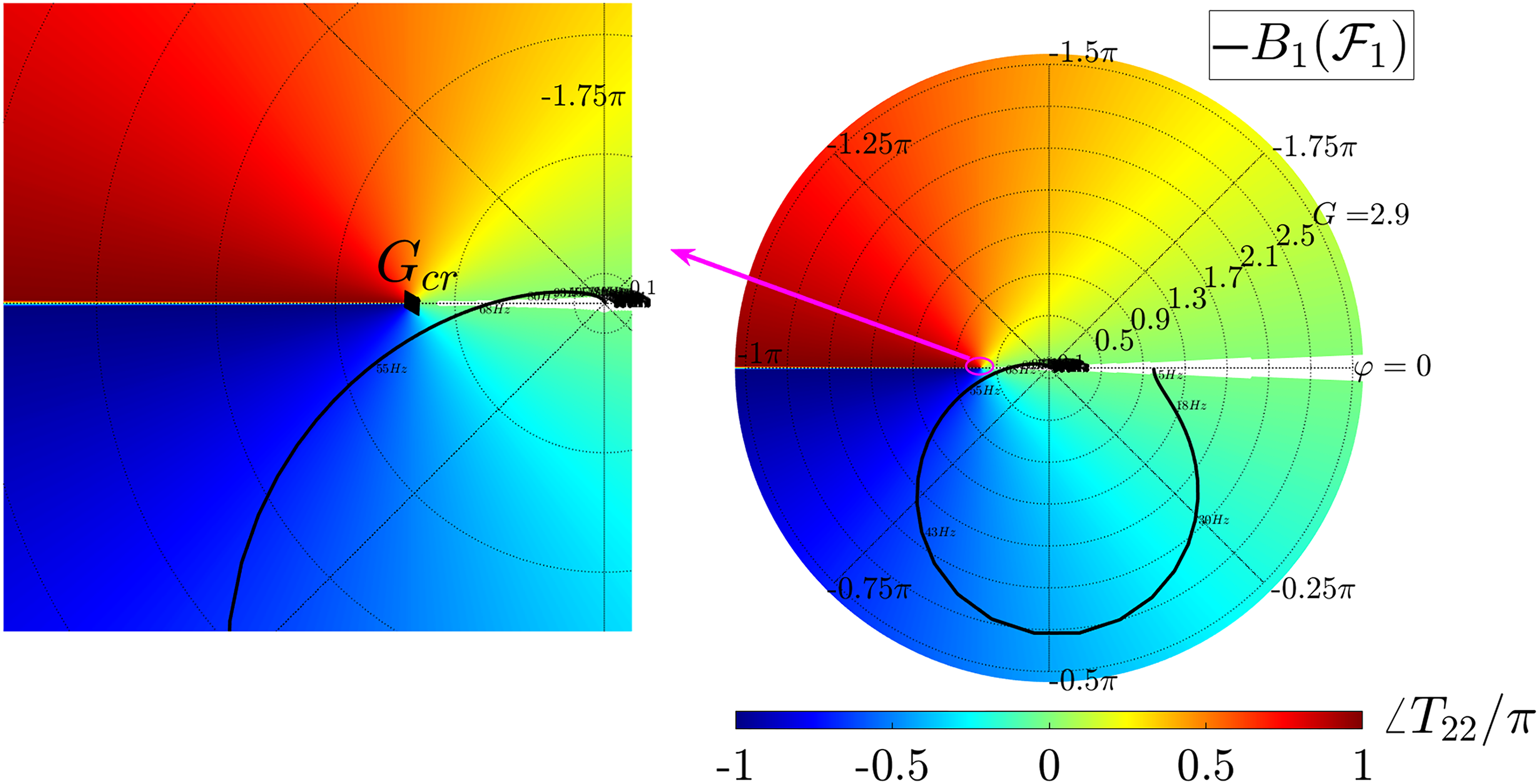
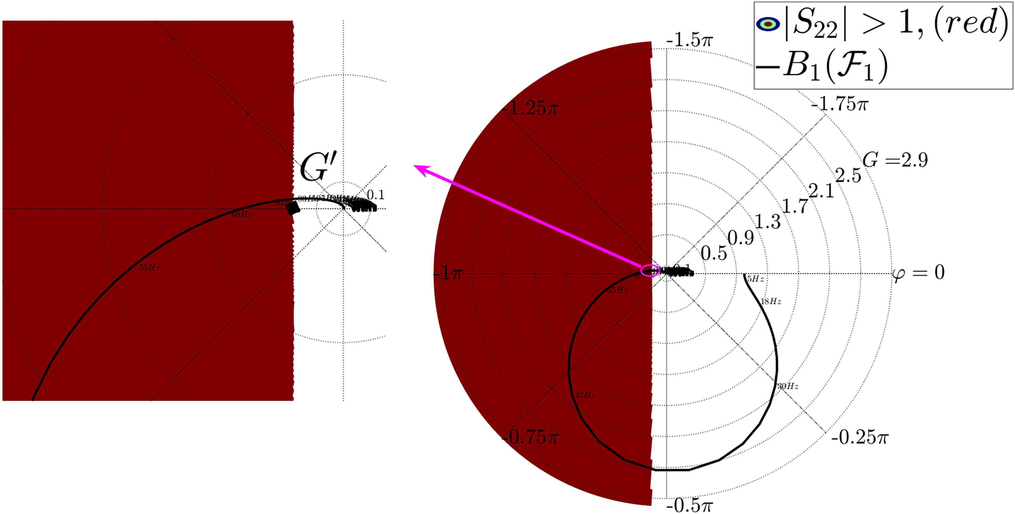
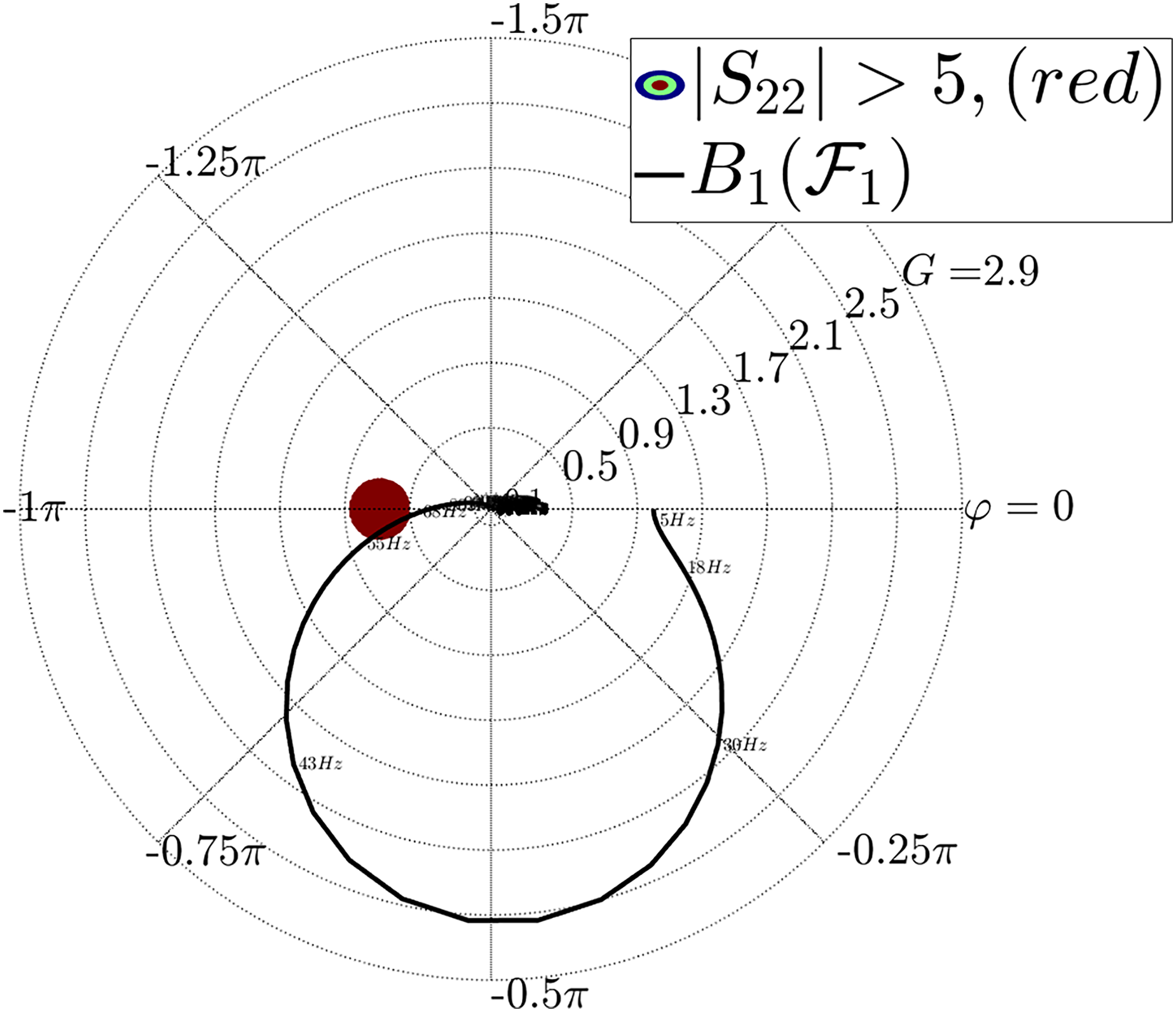
In Figure 10, the region where $|S_{22}|>1$ is highlighted in red, as evident, the critical region for the ITA mode ( $G>G_{cr}\approx 0.7$ ) with a phase crossing of $-\pi$ is entirely situated inside the red zone, as expected from equation (42). In addition, the sufficient condition to ensure $\mu >0$ is $G<G^{\prime }$ when $-0.5\pi <\phi <-1.5\pi$ . Returning to the details in the derivation of the $\mu$ criterion, it is evident that this formulation has been derived under the assumption of fully reflective terminations (i.e. $|R_{up}|=|R_{dn}|=1$ ), which represents the most critical condition in the absence of the unstable ITA mode. To demonstrate this, we visualize $S_{22}>1/|R_{dn}|$ in Figures 11 and 12 when $R_{dn}\ne 1$ . It can be observed that decreasing $|R_{dn}|$ leads to the critical (red) region, where the requirement for an infinite phase margin of $S_{11}$ and $S_{22}$ is violated, converging to the point $G=G_{cr}$ . Since we only consider flame TFs in the absence of the ITA mode, the gain at the frequency corresponding to the phase crossing of $-\pi$ is less than $G_{cr}$ , indicating that the case of fully reflective terminations (i.e. $|R_{up}|=|R_{dn}|=1$ ) is the most critical scenario for the risk of thermoacoustic instability.

Figure 11.

Evaluation of the scattering matrix coefficient $|R_{dn}\Vert S_{22}|$ with $|R_{dn}|=0.5$ .

Figure 12.

Evaluation of the scattering matrix coefficient $|R_{dn}\Vert S_{22}|$ with $|R_{dn}|=0.2$ .

Discussion on the limitation of $\mu$ and $k$ to be used as figure-of-merit

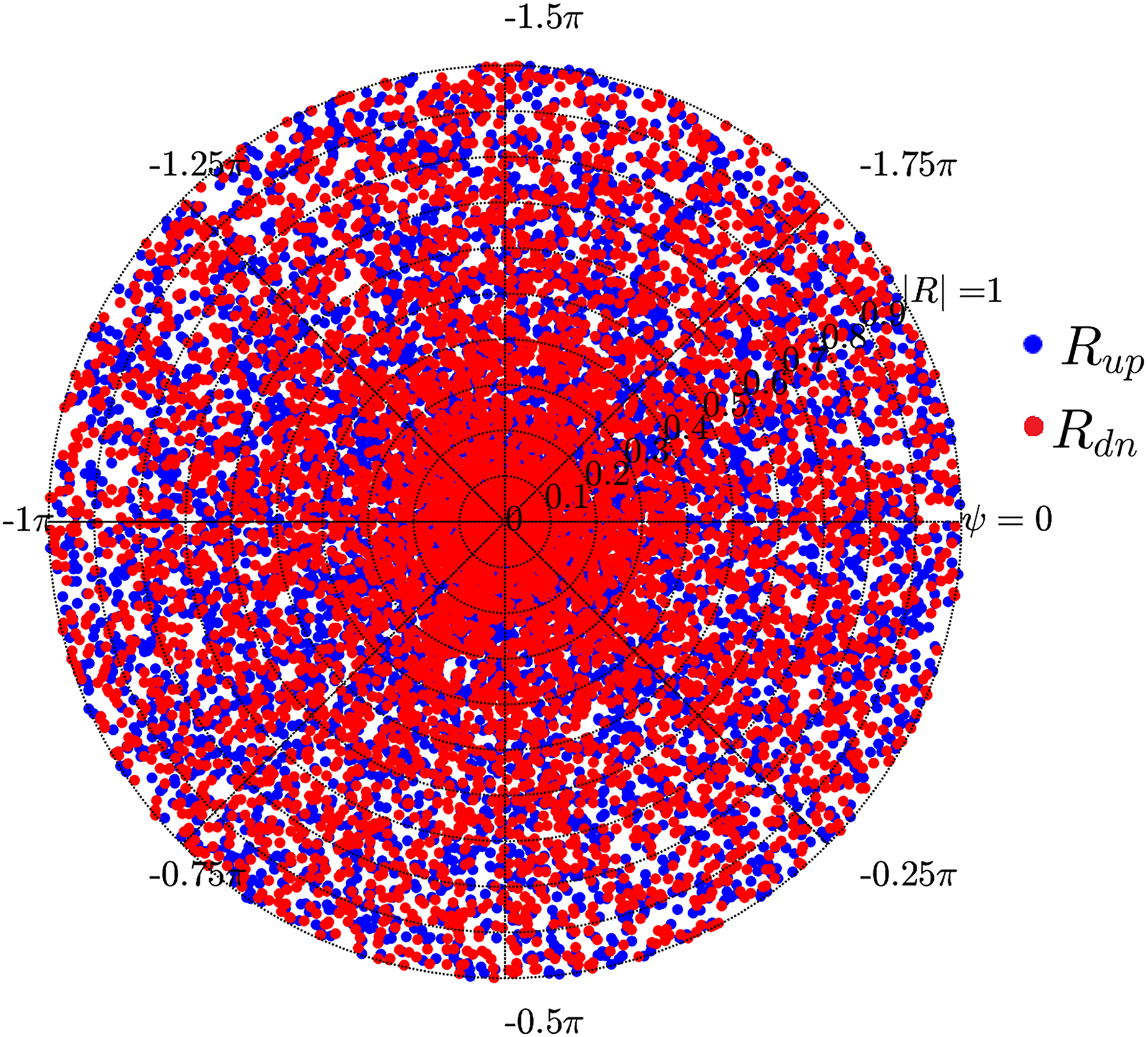
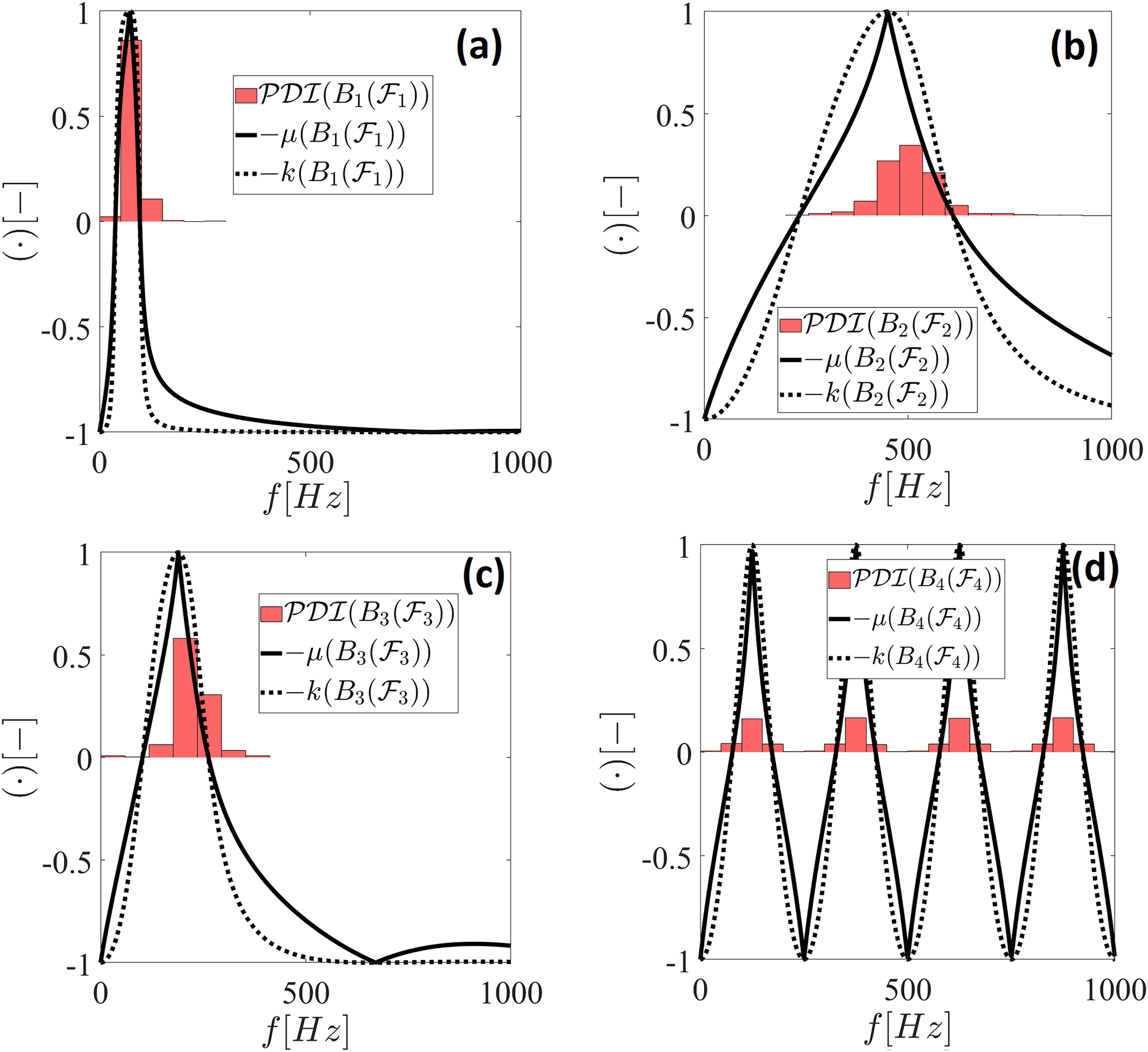
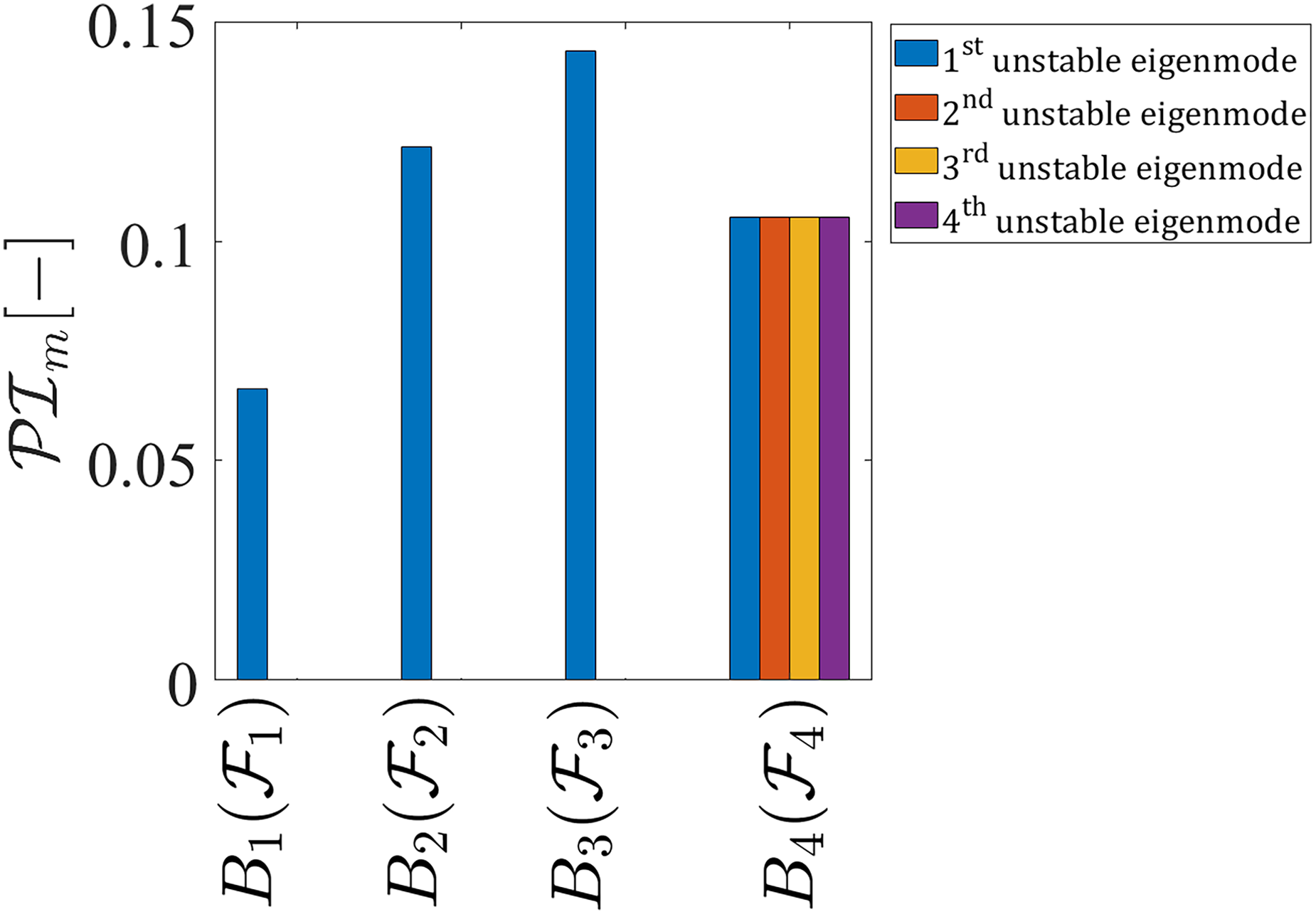
Having discussed the features and limitations of the $\mu$ and $k$ factors, we now explore their potential as quality factors in thermoacoustics (in the absence of pure unstable ITA mode) for comparing and ranking different burners. To address this question, a reference dataset is required for comparison. One possibility is to employ a MC simulation on solving the dispersion relation (equation (7)). In this simulation, a library of 5000 sets of frequency-independent passive upstream and downstream reflection coefficients is created uniformly and randomly distributed inside the unit complex circle (see Figure 13). Through an iterative MC simulation, the stability of the system equipped with the considered burners with flames in combinations with sets of upstream and downstream reflection coefficients can be calculated in numerous cases, enabling the determination of the probability of stability as $\mathcal{P}\mathcal{S}=N_u/N_t$ , where $N_u$ and $N_t$ are the number of unstable cases and the total number of cases, respectively. For more detailed description, see Kornilov and de Goey ¹⁰ and Saxena et al. ¹² . Figure 14 presents the histograms depicting the probability density of instability ( $\mathcal{P}\mathcal{D}\mathcal{I}$ ) versus unstable frequencies for different burners with flames. The distributions are compared with the $-\mu$ and $-k$ criteria, revealing a strong correspondence between the negative values of $\mu$ and $k$ and the concentration of unstable frequencies within a specific frequency range. It is worth noting that, as defined, the center of the unit circle represents the unsafe region, and the results provide indirect evidence that a more negative value of $\mu$ or $k$ corresponds to an enlarged unsafe area within the unit circle. This finding aligns with previous investigations conducted by Kornilov et al. ¹⁴ and Kojourimanesh et al. ¹⁵ . Furthermore, Figure 14(d) offers a clear visualization of how the $-\mu$ and $-k$ criteria effectively capture the distribution of unstable frequencies, even in scenarios where multiple unstable modes are present. Figure 15 shows the probability of instability concerning the number of unstable modes, which is defined as the ratio of the number of unstable cases to the total number of examined cases in the MC simulation. The results illustrate that $B_1({\mathcal{F}}_1)$ , $B_2({\mathcal{F}}_2)$ , and $B_3({\mathcal{F}}_3)$ have only one unstable eigenmode each. In contrast, $B_4({\mathcal{F}}_4)$ , which has been modeled with the $n-\tau$ model, exhibits multiple modes with equal probabilities. We here only evaluate first four unstable modes.

Figure 13.

Randomly generated upstream and downstream reflection coefficients as an input library for the Monte Carlo (MC) simulation.

Figure 14.

The histogram of distribution of unstable frequencies obtained from MC simulation, and a comparison with $-\mu$ and $-k$ criteria. The information on different flame TFs are given in Table 1. MC: Monte Carlo; TFs: transfer function.

Figure 15.

Probability of instability of different modes of the system for the four flame transfer functions (TFs) according to Table 1.

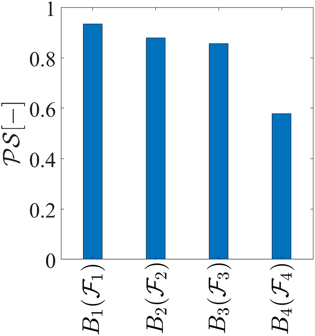
Figure 16 displays the overall probability of stability for different burners based on the MC simulations, allowing for easy comparison and ranking. Probability of stability can be obtained easily by calculating $\mathcal{P}\mathcal{S}=1-\mathcal{P}\mathcal{I}$ . Upon closer examination, it is evident that the $B_1({\mathcal{F}}_1)$ , $B_2({\mathcal{F}}_2)$ , and $B_3({\mathcal{F}}_3)$ show almost similar thermoacoustic quality. However, $B_1({\mathcal{F}}_1)$ slightly outperforms $B_2({\mathcal{F}}_2)$ and $B_3({\mathcal{F}}_3)$ , and $B_3({\mathcal{F}}_3)$ outperforms $B_4({\mathcal{F}}_4)$ . In this context, “better” implies a higher likelihood of thermoacoustic stability when combined with arbitrary sets of upstream/downstream embeddings.

Figure 16.

Total probability of stability of the system for burners with flames. The information on different flame transfer functions (TFs) are given in Table 1.

It is important to note that the performed MC simulation generated a library of constant (frequency-independent) uniformly random reflection coefficients, which represents a specific class of reflection coefficients. Therefore, it is not appropriate to generalize the obtained probability as a definitive measure. The MC simulation based on the constant reflection coefficients may indicate a good burner with a low probability of stability, but it is not possible to identify inherently bad burners with a high probability of stability. Keeping in mind, this limitation of the MC simulation, we can compare the burner ranking obtained from the MC simulation with that derived from the $\mu$ (or $k$ ) criterion.

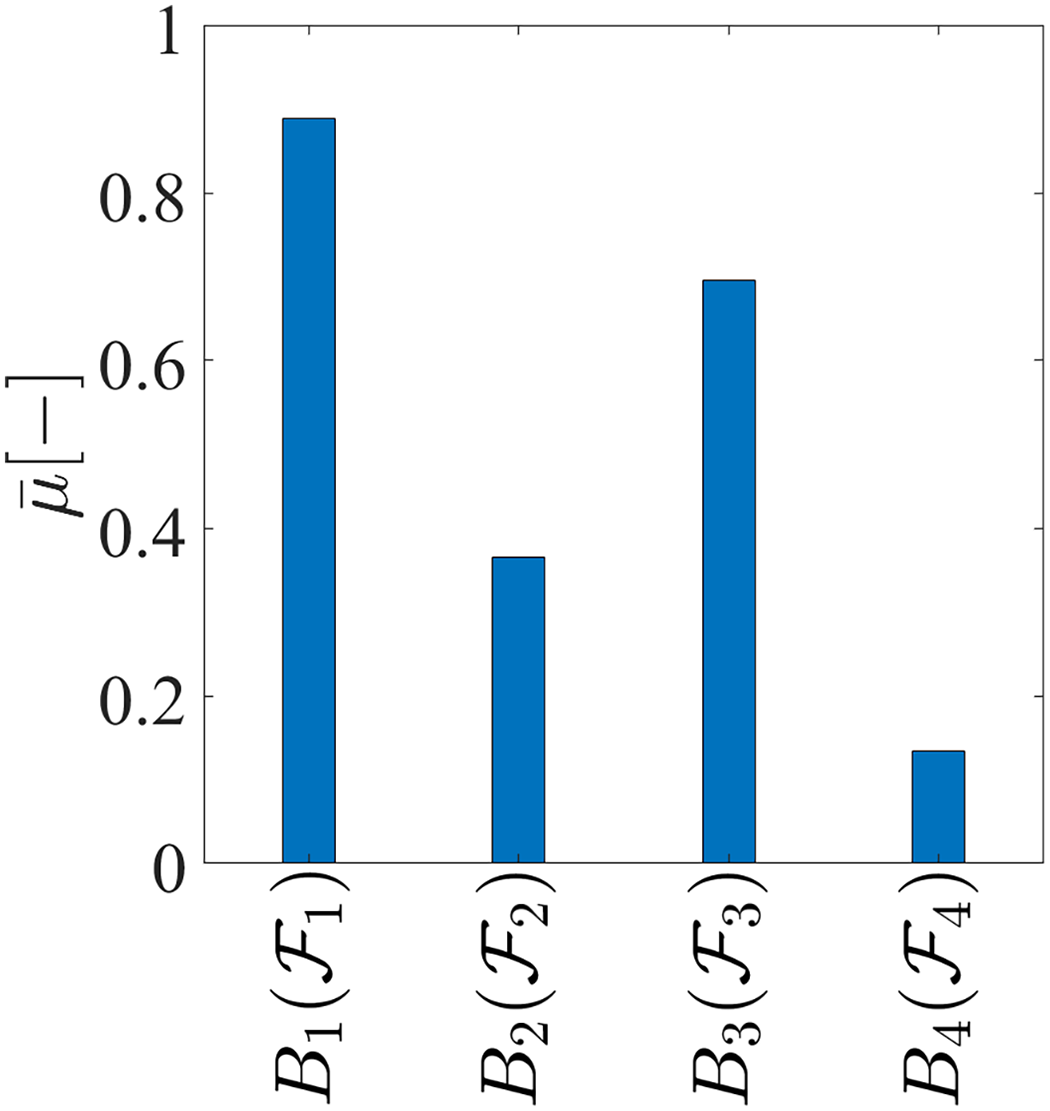
Figures 6 and 7 demonstrated that the variables $\mu$ and $k$ exhibit a strong dependence on the frequency and can qualitatively indicate the concentration of unstable frequencies. To compare the burners quantitatively, a single performance metric or quality factor needs to be calculated. The $\mu$ criterion represents the minimum distance to the unsafe region, where a higher value signifies a greater distance between the unsafe region and the origin, indicating a potentially safer operating condition. In order to obtain a single numerical value for each burner with a flame, the average $\mu$ value was computed over the entire frequency range, as depicted in Figure 17.

Figure 17.

The averaged value of $\mu$ to be used as figure-of-merit to rank different burners. The information on different flame transfer functions (TFs) are given in Table 1.

This averaging process facilitates a straightforward comparison among the burners, with higher average $\mu$ values may indicate a higher likelihood of thermoacoustic stability, and lower average $\mu$ values suggesting an increased risk of instability. Based on the rankings derived from the average $\mu$ values, the burners can be ranked in terms of their stability performance. $B_1({\mathcal{F}}_1)$ , possessing the highest average $\mu$ value, is considered superior to $B_3({\mathcal{F}}_3)$ . Similarly, $B_3({\mathcal{F}}_3)$ surpasses $B_2({\mathcal{F}}_2)$ due to its higher average $\mu$ value, indicating a more favorable stability profile. Finally, $B_2({\mathcal{F}}_2)$ exhibits a higher average $\mu$ value compared to $B_4({\mathcal{F}}_4)$ , thereby suggesting a better likelihood of stability. Upon comparing the results of the $\mu$ criterion with the MC simulation, it is worth noting that the ranking of burners based on the $\mu$ criterion does not align with the ranking based on the MC simulation. Specifically, burner 2, which is identified as the second-best burner according to the MC simulation with slight thermoacoustic difference with burner 1 and burner 3, does not exhibit the second-highest $\mu$ value. This discrepancy can be attributed to the fact that the $\mu$ criterion heavily relies on the concept of unconditional stability of subsystem (e.g. input reflection coefficient).

Upon closer examination of the flame TF of $B_2({\mathcal{F}}_2)$ in Figure 5, it is apparent that its phase gradually decreases over a wide frequency range, remaining around $-\pi$ . Consequently, the $\mu$ value for $B_2({\mathcal{F}}_2)$ in Figure 7 is significantly negative. This behavior can lead to a misleading ranking when using the $\mu$ criterion, particularly for burners whose flame TF saturates around $-\pi$ , almost irrespective of their gain values. A similar conclusion can be drawn for the $k$ criterion as well.

Moreover, when comparing $B_2({\mathcal{F}}_2)$ and $B_3({\mathcal{F}}_3)$ based on the MC simulation, it is observed that they exhibit quite similar probabilities of stability. However, the $\mu$ criterion shows a significant difference between them, potentially leading to a misleading ranking. Additionally, the $\mu$ criterion suggests that $B_4({\mathcal{F}}_4)$ has a high risk of instability, while the MC simulation demonstrates that it may actually operate acoustically stable in $\sim$ 60% of the situations. This discrepancy highlights the limitations of the $\mu$ criterion in accurately predicting the thermoacoustic stability of burners. In summary, the concept of infinite phase margin and unconditional stability of subsystem, which underlie the $\mu$ and $k$ criteria, yield very conservative quality factors that can mislead to evaluate properly thermoacoustic quality of burners with their associated flames, even in the absence of pure unstable ITA mode. Nevertheless, they can still qualitatively identify the frequency range of potential instability correctly.

Conclusion

This study addressed the challenge of evaluating the thermoacoustic performance of burners and their associated flames in the absence of information about specified upstream or downstream acoustics. The concept of a figure-of-merit for burners was explored, with the $\mu$ and $k$ factors from microwave theory proposed as potential candidates. While the $\mu$ and $k$ factors demonstrate the capability to accurately predict the distribution of unstable frequencies, their use as quantitative metrics for burner evaluation was cautioned against. Through comprehensive analysis, it was revealed that these factors suffer from limitations and not always valid assumptions when applied in the context of thermoacoustics, rendering them less suitable as figure-of-merit for burners. Three key limitations of these criteria are as follows:

The $\mu$ and $k$ criteria are formulated under the assumption that the $S$ -parameters do not have any RHP poles. Consequently, these criteria cannot be applied in the presence of an unstable ITA mode.

The $\mu$ criterion measures the minimum distance from the center of the complex unit circle. While this measure is sufficient for checking unconditional stability, achieving unconditional stability across the entire frequency range is often not feasible in thermoacoustic applications.

The requirement for unconditional stability imposes an overly conservative constraint, rendering it an unreliable performance metric in thermoacoustics.

It is also important to note that while the MC simulation based on frequency-independent reflection coefficient has been utilized in this study to demonstrate the inefficiency and limitations of the $\mu$ and $k$ criteria, it should not be concluded that this form of the MC simulation is a universally applicable solution for determining a quality factor to compare different burners. Instead, this research emphasizes the need for alternative methodologies to effectively assess the thermoacoustic quality of burners and their associated flames when upstream or downstream acoustics are unspecified. Future studies should focus on the development of new metrics or approaches that can provide a comprehensive evaluation of thermoacoustic performance and stability, thereby offering valuable insights for the design and optimization of combustion systems.