Iterative solvers for the thermoacoustic nonlinear eigenvalue problem and their convergence properties

Abstract

The spectrum of the thermoacoustic operator is governed by a nonlinear eigenvalue problem. A few different strategies have been proposed by the thermoacoustic community to tackle it and identify the frequencies and growth rates of thermoacoustic eigenmodes. These strategies typically require the use of iterative algorithms, which need an initial guess and are not necessarily guaranteed to converge to an eigenvalue. A quantitative comparison between the convergence properties of these methods has however never been addressed. By using adjoint-based sensitivity, in this study we derive an explicit formula that can be used to quantify the behaviour of an iterative method in the vicinity of an eigenvalue. In particular, we employ Banach’s fixed-point theorem to demonstrate that there exist thermoacoustic eigenvalues that cannot be identified by some of the iterative methods proposed in the literature, in particular fixed-point iterations, regardless of the accuracy of the initial guess provided. We then introduce a family of iterative methods known as Householder’s methods, of which Newton’s method is a special case. The coefficients needed to use these methods are explicitly derived by means of high-order adjoint-based perturbation theory. We demonstrate how these methods are always guaranteed to converge to the closest eigenvalue, provided that the initial guess is accurate enough. We also show numerically how the basin of attraction of the eigenvalues varies with the order of the employed Householder’s method.

Introduction

Thermoacoustic instabilities can be assessed by solving the inhomogeneous Helmholtz equation

$$\mathrm{\nabla }\cdot \left(c^2\mathrm{\nabla }\hat{p}\right)+{\omega }^2\hat{p}=(c_2^2-c_1^2)n(\mathit{x})e^{-\mathrm{i}\omega \tau }{\mathrm{\nabla }\hat{p}|}_{{\mathit{x}}_{\mathbf{r}\mathbf{e}\mathbf{f}}}$$

(1)

on a prescribed geometry with appropriate boundary conditions. ¹ In Eq. (1) $\hat{p}$ indicates the complex-valued amplitude of the Fourier transform of the pressure fluctuations (the eigenfunction) and $c$ the speed of sound, with the subscripts ${}_1$ and ${}_2$ indicating the regions upstream and downstream the flame, respectively. The interaction index $n$ , which is non-zero only over an acoustically compact volume, and the time delay $\tau$ model the flame response.^2,3 Equation (1) defines a nonlinear eigenvalue problem (NLEVP) in the complex frequency $\omega$ . Once discretized, e.g. by means of finite elements, the NLEVP can be expressed in compact form as

$$\mathsf{L}(\omega )\mathit{p}=\mathbf{0}\mathbf{,}$$

(2)

where $\mathbf{L}$ is an $N\times N$ large, sparse matrix depending nonlinearly on $\omega$ . Although there exist efficient algorithms to solve generalized linear eigenvalue problems, for which $\mathbf{L}(\omega )=(\mathbf{X}-\omega \mathbf{Y})$ , solving an eigenvalue problem that is nonlinear in the eigenvalue $\omega$ is intrinsically harder.^4–6 A typical approach is to transform the NLEVP into a (series of) associated eigenvalue problems linear in the eigenvalue. For example:

• NLEVPs that are polynomial in $\omega$ with order $K$ can be recast into linear eigenvalue problems of dimension $KN$ ³ ;

• Solutions of NLEVPs can be found by iteratively solving linear eigenvalue problems resulting from the expansion of $\mathbf{L}(\omega )$ (to any desired order) in the eigenvalue ⁶ ;

• Contour integration methods reduce the NLEVP to a linear eigenvalue problem possessing only the eigenvalues of $\mathbf{L}$ inside a given contour in the complex plane.^7,8

These approaches exploit the fact that efficient and robust methods (e.g. Arnoldi) exist for large scale linear eigenvalue problems.^9,10A common feature of iterative methods is that they all require an initial guess ${\omega }_1$ for the eigenvalue ^a , which is updated at every iteration. Eigenvalues of the thermoacoustic operator are fixed points of the mapping defined by the chosen iterative algorithm.

According to Banach’s fixed-point theorem ¹¹ p. 152, for an iterative algorithm to be able to identify an eigenvalue, the mapping defined by the algorithm needs to be contracting in the vicinity of the eigenvalue. This means that, provided that the initial guess is sufficiently close to an eigenvalue, at each iteration the algorithm will move the guess closer to the eigenvalue, until a prescribed tolerance is reached. On the other hand, if the mapping is repelling in the vicinity of an eigenvalue, it will not be possible to identify this eigenvalue with the chosen algorithm, since a sufficiently close guess will be pushed further away from the solution. An overlooked eigenvalue can have serious consequences in thermoacoustics, as the reliable and accurate determination of all relevant ^b eigenvalues is of paramount importance to ensure the safe operability of an engine.

The fixed-point iteration method described in ³ is a commonly used algorithm for identifying eigenvalues of the thermoacoustic Helmholtz operator – it is used in^12–17 to name a few. However, with the exception of a short discussion in, ¹² there is no reference in the literature investigating the convergence properties of this method in relation to the spectrum of the thermoacoustic operator. The aim of this work is to quantify the convergence properties of fixed-point iteration methods that are commonly used in thermoacoustics. It will be shown that some thermoacoustic eigenvalues cannot be found using a fixed-point algorithm, regardless of the chosen initial guess. We will then introduce an alternative adjoint-based iterative method that has more robust convergence properties and is thus better suited to tackle the thermoacoustic problem.

This study is organized as follows. First the thermoacoustic problem and the fixed-point iteration presented in ³ are introduced. An explicit formula that quantifies the convergence properties of the fixed-point mapping is derived. The same procedure is conducted for a so-called Picard iteration, which is another form of fixed-point iteration. Both methods are applied to a generic thermoacoustic test case to demonstrate that some eigenvalues are repellors with respect to these mappings. We will then introduce a class of adjoint-based solution methods known as Householder, of which Newton’s method is a special case. It will be discussed how all eigenvalues of the thermoacoustic operator are attractors with respect to these solution methods, and how the basins of attraction of each eigenvalue vary depending on the order of the Householder’s method used.

The thermoacoustic nonlinear eigenvalue problem

The weak formulation and discretization of the thermoacoustic Helmholtz equation (1) results in an $N$ -dimensional NLEVP that reads

$$\mathbf{L}(\omega )\mathit{p}=(\mathbf{K}+\omega \mathbf{C}+{\omega }^2\mathbf{M}+\mathbf{Q}(\omega ))\mathit{p}=\mathbf{0}.$$

(3)

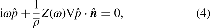
The matrices in (3) arise from discretizing the operators in equation (1), viz. the stiffness operator $\mathrm{\nabla }\cdot (c^2\mathrm{\nabla }(\cdot ))\mapsto \mathbf{K}$ , the mass operator ${\omega }^2(\cdot )\mapsto {\omega }^2\mathbf{M}$ , and the flame operator $-(c_2^2-c_1^2)n(\mathit{x})e^{-i\omega \tau }\mathrm{\nabla }{|}_{{\mathit{x}}_{\mathrm{ref}}}(\cdot )\mapsto \mathbf{Q}(\omega )$ . The matrix $\mathbf{C}$ results from the discretization of the boundary conditions needed to close the problem. They can be expressed in terms of the acoustic impedance $Z$ on all boundaries

$$\mathrm{i}\omega \hat{p}+\frac{1}{\overline{\rho }}Z(\omega )\mathrm{\nabla }\hat{p}\cdot \hat{\mathit{n}}=0,$$

(4)

where $\hat{\mathit{n}}$ is a unit vector normal to the boundary.

Equation (3) represents a nonlinear eigenvalue problem. The challenge is to find all its eigenvalues $\omega$ – and their corresponding eigenvectors $\mathit{p}$ – in a prescribed portion of the complex plane.

Rijke tube test-case

Throughout this study we will employ the classic Rijke tube configuration ¹⁸ to demonstrate our results. It consists of a straight duct in which a flame is located. Across the flame the temperature, and hence the speed of sound, rise abruptly. The axial flame location $x_{\mathrm{f}}$ is chosen to be in the middle of the tube. The parameters that determine the acoustic response of the system are chosen to be identical to those used in. ³ By non-dimensionalizing all quantities using the tube length $L$ as a characteristic length and the speed of sound $c_1$ in the cold section of the duct as a characteristic velocity, the chosen Rijke tube’s parameter are $x_{\mathrm{f}}=0.5$ , $c(x)=1$ for $x\le x_{\mathrm{f}}$ and $c(x)=2$ otherwise. The boundary conditions are chosen to be acoustically closed ( $\mathrm{\nabla }\hat{p}=0$ ) and opened ( $\hat{p}=0$ ) at the inlet ( $x=0$ ) and outlet ( $x=1$ ), respectively. The flame model parameters are chosen to be $n=1/3$ and $\tau =2$ .

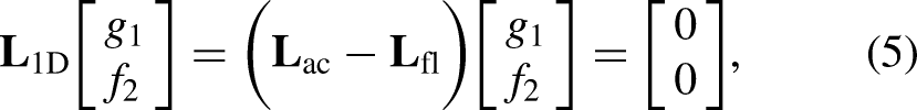
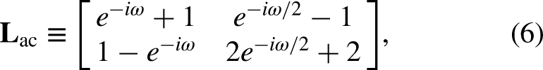
For the range of frequencies that we will consider all transverse modes are cut-off. The problem can therefore be considered as one-dimensional, and the flame to be a point source in the Helmholtz equation (1), $n(x)=n\delta (x-x_{\mathrm{f}})$ . The eigenvalues of this problem can be calculated semi-analytically by using an acoustic network approach. ¹⁸ By assuming one-dimensional acoustics, equation (1) can be expressed in terms of the Riemann invariants $f$ and $g$ . With suitable matching conditions at the flame zone and for the parameters introduced above, the acoustic-network eigenvalue problem reads ¹⁹

$${\mathbf{L}}_{1\mathrm{D}}\left[\begin{array}{c}{g}_1\\ f_2\end{array}\right]=({\mathbf{L}}_{\mathrm{ac}}-{\mathbf{L}}_{\mathrm{fl}})\left[\begin{array}{c}{g}_1\\ f_2\end{array}\right]=\left[\begin{array}{c}0\\ 0\end{array}\right],$$

(5)

where ${\mathbf{L}}_{\mathrm{ac}}$ is the acoustic response in the absence of an active flame

$${\mathbf{L}}_{\mathrm{ac}}\equiv \left[\begin{array}{cc}{e}^{-i\omega }+1& e^{-i\omega /2}-1\\ 1-e^{-i\omega }& 2e^{-i\omega /2}+2\end{array}\right],$$

(6)

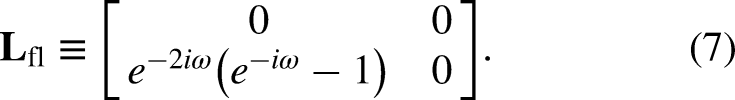
and ${\mathbf{L}}_{\mathrm{fl}}$ provides the feedback between heat release rate fluctuations and the acoustics

$${\mathbf{L}}_{\mathrm{fl}}\equiv \left[\begin{array}{cc}0& 0\\ e^{-2i\omega }(e^{-i\omega }-1)& 0\end{array}\right].$$

(7)

By imposing det $({\mathbf{L}}_{1\mathrm{D}})=0$ the eigenvalues of the Rijke tube can be obtained by using standard root-finder methods. We shall focus our analysis on the properties of the four thermoacoustic eigenvalues found in the region $\mathcal{S}$ of the complex plane delimited by

$$\mathcal{S}=\{\omega \mid \mathrm{\Re }(\omega )\in [0,10]\wedge \mathrm{\Im }(\omega )\in [-1,1]\},$$

(8)

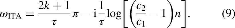
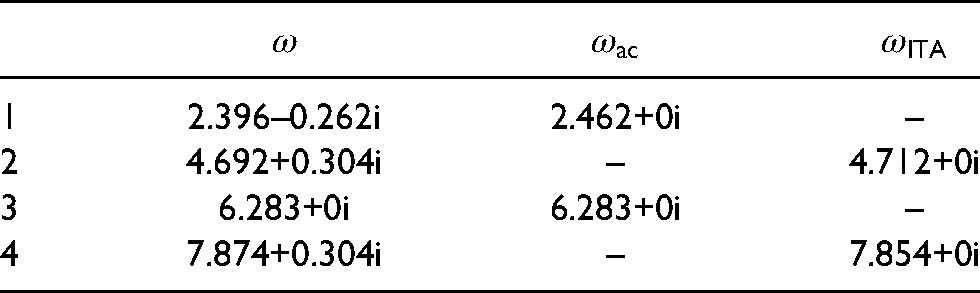
which are reported in Table 1. Two of these eigenvalues can be linked to acoustic modes – whose eigenvalues ${\omega }_{\mathrm{ac}}$ can be calculated by setting $n=0$ , which implies ${\mathbf{L}}_{\mathrm{fl}}\mathbf{=}\mathsf{0}$ – while the other two can be linked to intrinsic thermoacoustic (ITA) modes – whose frequencies are given by^20,21

$${\omega }_{\mathrm{ITA}}=\frac{2k+1}{\tau }\pi -\mathrm{i}\frac{1}{\tau }\log \left[(\frac{c_2}{c_1}-1)n\right].$$

(9)

Table 1.

Eigenvalues of the Rijke tube network model (5) in the considered portion of the complex plane together with the associated acoustic (no flame) and intrinsic (anechoic boundary conditions) eigenvalues from which they stem.

	$\omega$	${\omega }_{\mathrm{ac}}$	${\omega }_{\mathrm{ITA}}$
1	2.396–0.262 $\mathrm{i}$	2.462+0 $\mathrm{i}$	–
2	4.692+0.304 $\mathrm{i}$	–	4.712+0 $\mathrm{i}$
3	6.283+0 $\mathrm{i}$	6.283+0 $\mathrm{i}$	–
4	7.874+0.304 $\mathrm{i}$	–	7.854+0 $\mathrm{i}$

In the following, we will discretize by finite elements the thermoacoustic eigenproblem (3) and use various iterative solution techniques to identify its eigenvalues. The semi-analytical wave-based solutions presented in Table 1 will serve as benchmarks. The dimensions of the resulting matrix operator $\mathbf{L}$ do not allow for the use of determinant-based methods, and alternative iterative strategies are needed.

State-of-the-art iterative solution method

A fixed-point iteration to solve the NLEVP (3) was proposed in. ³ This algorithm exploits the fact that the problem is quadratic in $\omega$ , except for the heat release term. ^c The flame operator can therefore be thought of as a perturbation of the underlying purely acoustic problem, which is obtained with $\mathbf{Q}\mathbf{=}\mathbf{0}$ . This motivates the use of an iterative strategy, starting from the (known) purely acoustic solutions.

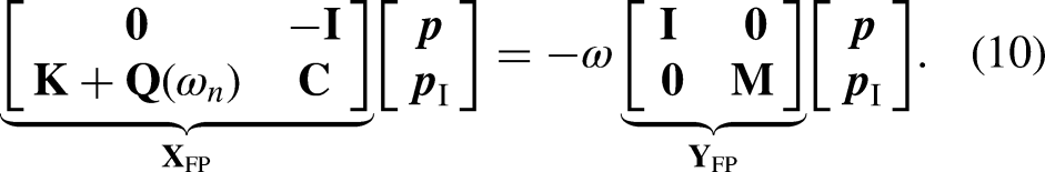
The key idea is to recast the problem into a linear eigenvalue problem of doubled dimension, and then to iteratively identify a thermoacoustic eigenvalue starting from an initial guess. We shall indicate this linear eigenvalue problem as ${\mathbf{L}}_{\mathrm{FP}}({\omega }_n;\omega )\tilde{\mathit{p}}=0$ . It reads

$$\underset{{\mathbf{X}}_{\mathrm{FP}}}{\underbrace{\left[\begin{array}{cc}\mathbf{0}& -\mathbf{I}\\ \mathbf{K}+\mathbf{Q}({\omega }_n)& \mathbf{C}\end{array}\right]}}\left[\begin{array}{c}\mathit{p}\\ {\mathit{p}}_{\mathrm{I}}\end{array}\right]=-\omega \underset{{\mathbf{Y}}_{\mathrm{FP}}}{\underbrace{\left[\begin{array}{cc}\mathbf{I}& \mathsf{0}\\ \mathsf{0}& \mathbf{M}\end{array}\right]}}\left[\begin{array}{c}\mathit{p}\\ {\mathit{p}}_{\mathrm{I}}\end{array}\right].$$

(10)

On the left hand side, the nonlinear dependency of the problem on the eigenvalue has been removed by freezing the evaluation of the flame operator $\mathbf{Q}$ , i.e, by evaluating at ${\omega }_n$ , the eigenvalue guess. This guess is updated by iteratively replacing ${\omega }_n$ with the closest eigenvalue $\omega$ of (10), which can be found by means of, e.g., the Arnoldi iteration method. The eigenvector in (10) has been extended into

$$\tilde{\mathit{p}}=[\mathit{p},\omega \mathit{p}].$$

(11)

This can be seen from the first matrix equation defined by (10), which reads ${\mathit{p}}_{\mathrm{I}}=\omega \mathit{p}$ . By using this relation, the second matrix equation of (10) reduces to (3) when ${\omega }_n=\omega$ . The algorithm terminates successfully if the difference between the results of two successive iterations is less than a prescribed tolerance ${\mathrm{tol}}_{\omega }$ , or is aborted if a predefined maximum number of iterations is reached.

Algorithm 1

Nicoud’s algorithm

1: function ITERATE( ${\omega }_1,{\mathit{p}}_1,{\mathrm{tol}}_{\omega },\mathrm{maxiter},\mathbf{K}\mathbf{,}\mathbf{C}\mathbf{,}\mathbf{M}\mathbf{,}\mathbf{Q}$ )

2:  ${\omega }_0\leftarrow \mathrm{\infty }$

3:  $n\leftarrow 1$

4:  ${\tilde{\mathit{p}}}_1\leftarrow \left[\begin{array}{c}{\mathit{p}}_{\mathrm{I}}\\ {\omega }_1{\mathit{p}}_1\end{array}\right]$

5:  ${\mathbf{Y}}_{\mathrm{FP}}\leftarrow \left[\begin{array}{cc}\mathbf{I}& \mathbf{0}\\ \mathbf{0}& \mathbf{M}\end{array}\right]$

6: while $|{\omega }_n-{\omega }_{n-1}|>{\mathrm{tol}}_{\omega }$ and $n<\mathrm{maxiter}$ do

7:    ${\mathbf{X}}_{\mathrm{FP}}\leftarrow \left[\begin{array}{cc}\mathbf{0}& -\mathbf{I}\\ \mathbf{K}\mathbf{+}\mathbf{Q}\mathbf{(}{\omega }_{\mathbf{n}}\mathbf{)}& \mathbf{C}\end{array}\right]$

8:    ${\mathit{\omega }}_{n+1},{\tilde{\mathit{p}}}_{n+1}\leftarrow \mathrm{EIGS}(-{\mathbf{X}}_{\mathrm{FP}},{\mathbf{Y}}_{\mathrm{FP}},{\omega }_n,{\tilde{\mathit{p}}}_n)$

9:    $n\leftarrow n+1$

10: end while

11:  ${\mathit{p}}_n\leftarrow {\tilde{\mathit{p}}}_n[1:N]$

12: return ${\omega }_n,{\mathit{p}}_n,n$

13: end function

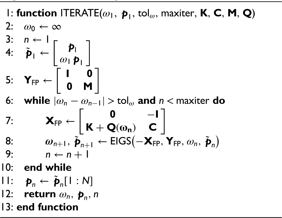
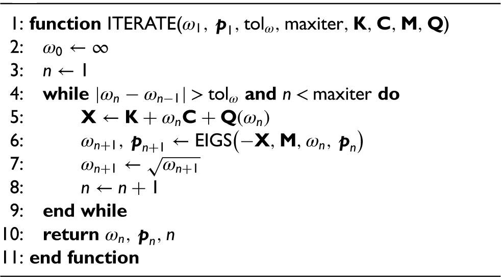
The pseudocode for the fixed-point iterative scheme is outlined in Alg. 1. We have denoted with $\mathrm{EIGS}(\mathbf{X},\mathbf{Y},{\omega }_1,{\mathit{p}}_1)$ the Arnoldi method that identifies the eigenpair $\omega ,\mathit{p}$ of the linear eigenvalue problem $\mathbf{X}p=\omega \mathbf{Y}p$ closest to ${\omega }_1$ . An initial guess for the eigenvector ${\mathit{p}}_1$ , if known, may also be provided to the algorithm, in order to improve the convergence of the Arnoldi method. Also note that the matrix $\mathbf{M}$ is always positive-definite – as it defines a mass matrix – and hence is ${\mathbf{Y}}_{\mathrm{FP}}$ . Thus, the eigenvalue problem $({\mathbf{X}}_{\mathrm{FP}}({\omega }_n)-\omega {\mathbf{Y}}_{\mathrm{FP}})\tilde{\mathit{p}}=\mathbf{0}$ appearing at each iteration, can be solved efficiently.

Fixed-point iteration schemes in thermoacoustics

A single iteration of the procedure described in Alg. 1 defines a mapping ${\omega }_{n+1}=f({\omega }_n)$ for which fixed-points $\omega$ are sought. This fixed-point map $f$ can be explicitly expressed by rewriting the eigenvalue problem (10) as

$${\mathbf{L}}_{\mathrm{FP}}(f;{\omega }_n)\tilde{\mathit{p}}=({\mathbf{X}}_{\mathrm{FP}}({\omega }_n)+f{\mathbf{Y}}_{\mathrm{FP}})\tilde{\mathit{p}}=\mathbf{0}\mathbf{.}$$

(12)

A condition for the convergence of the mapping to an eigenvalue of the thermoacoustic operator is provided by Banach’s fixed-point theorem, which we briefly recall. Consider a bounded domain $\mathrm{\Gamma }\subset \mathbb{C}$ that contains the fixed-point $\omega$ . Banach’s fixed-point theorem guarantees that $f$ has one (unique) fixed-point in $\mathrm{\Gamma }$ as long as $f$ is a contraction everywhere in $\mathrm{\Gamma }$ .

For our purposes, we are only interested at the behaviour of the iterative map at the fixed-point. In particular, to know if an eigenvalue $\omega$ is an attractor of a given iterative method $f$ it is sufficient to verify that

$$|f^{\prime }(\omega )|<1.$$

(13)

This in fact implies that the mapping $f$ represents a contraction in the vicinity of $\omega$ . Provided that Eq. (13) is satisfied, the eigenvalue $\omega$ can be found if the initial guess lies sufficiently close to it.

Nicoud ³ recognized the importance of the contraction properties of $f$ , but stated that “[ …] obtaining general results about the contracting properties of the operator $f$ from physical arguments is out of reach of the current understanding of the thermoacoustic instabilities.” Significant progress has been made in this direction by the thermoacoustic community in recent years, and tools are now available to quantify the behaviour of the mapping $f$ from the thermoacoustic equations. In particular, the contraction properties of the mapping $f$ can be quantified by exploiting adjoint-based sensitivity.^22,23 In the following, we use adjoint methods to derive an analytical expression that allows us to compute $|f^{\prime }(\omega )|$ and thus make explicit use of Banach’s theorem.

Contraction properties of the fixed-point iteration

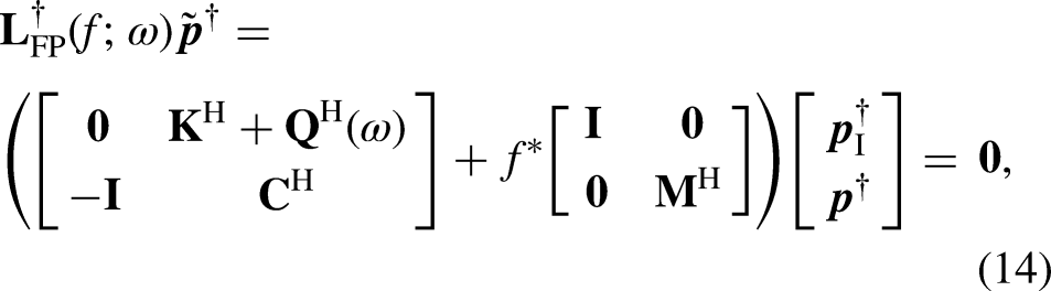
The adjoint equation associated with the mapping (12) reads:

$$\begin{array}{rl}& {\mathbf{L}}_{\mathrm{FP}}^{†}(f;\omega ){\tilde{\mathit{p}}}^{†}=\\ & (\left[\begin{array}{cc}\mathsf{0}& {\mathbf{K}}^{\mathrm{H}}+{\mathbf{Q}}^{\mathrm{H}}(\omega )\\ -\mathbf{I}& {\mathbf{C}}^{\mathrm{H}}\end{array}\right]+f^{*}\left[\begin{array}{cc}\mathbf{I}& \mathsf{0}\\ \mathsf{0}& {\mathbf{M}}^{\mathrm{H}}\end{array}\right])\left[\begin{array}{c}{\mathit{p}}_{\mathrm{I}}^{†}\\ {\mathit{p}}^{†}\end{array}\right]=\mathbf{0}\mathbf{,}\end{array}$$

(14)

where $f^{*}$ denotes the complex conjugate of $f$ . Its fixed-points are found when $f^{*}={\omega }^{*}$ . The second matrix equation defined by (14) shows that ${\mathit{p}}_{\mathrm{I}}^{†}=({\mathbf{C}}^{\mathrm{H}}+{\omega }^{*}{\mathbf{M}}^{\mathrm{H}}){\mathit{p}}^{†}$ , so that the extended adjoint eigenvector ${\tilde{\mathit{p}}}^{†}$ satisfies

$${\tilde{\mathit{p}}}^{†}={[({\mathbf{C}}^{\mathrm{H}}+{\omega }^{*}{\mathbf{M}}^{\mathrm{H}}){\mathit{p}}^{†},{\mathit{p}}^{†}]}^{\mathrm{T}}.$$

(15)

The first matrix equation in (14) defines the adjoint eigenvalue problem ${\mathbf{L}}^{†}(\omega ){\mathit{p}}^{†}=\mathbf{0}$ .

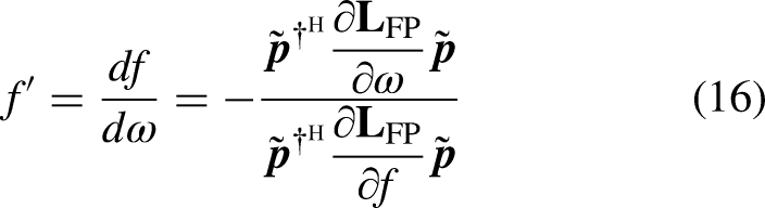
From adjoint-based sensitivity analysis, the following formula is known for evaluating the derivative of $f$ with respect to $\omega$ ^22,23:

$$f^{\prime }=\frac{df}{d\omega }=-\frac{{\tilde{\mathit{p}}}^{{†}^{\mathrm{H}}}\frac{\mathrm{\partial }{\mathbf{L}}_{\mathrm{FP}}}{\mathrm{\partial }\omega }\tilde{\mathit{p}}}{{\tilde{\mathit{p}}}^{{†}^{\mathrm{H}}}\frac{\mathrm{\partial }{\mathbf{L}}_{\mathrm{FP}}}{\mathrm{\partial }f}\tilde{\mathit{p}}}$$

(16)

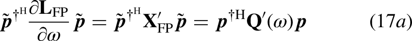
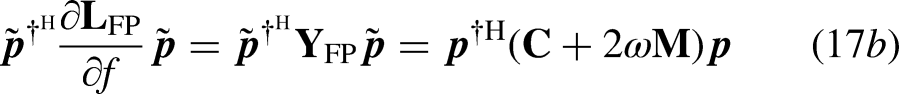
By combining the known information on the direct and adjoint eigenvectors – Eqs. (11) and (15), respectively – as well as on the functional shape of ${\mathbf{L}}_{\mathrm{FP}}$ – Eqs. (12) and (10) – we have

$${\tilde{\mathit{p}}}^{{†}^{\mathrm{H}}}\frac{\mathrm{\partial }{\mathbf{L}}_{\mathrm{FP}}}{\mathrm{\partial }\omega }\tilde{\mathit{p}}={\tilde{\mathit{p}}}^{{†}^{\mathrm{H}}}{\mathbf{X}}_{\mathrm{FP}}^{\mathrm{\prime }}\tilde{\mathit{p}}={\mathit{p}}^{†\mathrm{H}}{\mathbf{Q}}^{\mathrm{\prime }}(\omega )\mathit{p}$$

(17a)

$${\tilde{\mathit{p}}}^{{†}^{\mathrm{H}}}\frac{\mathrm{\partial }{\mathbf{L}}_{\mathrm{FP}}}{\mathrm{\partial }\mathbf{f}}\tilde{\mathit{p}}={\tilde{\mathit{p}}}^{{†}^{\mathrm{H}}}{\mathbf{Y}}_{\mathrm{FP}}\tilde{\mathit{p}}={\mathit{p}}^{†\mathrm{H}}(\mathbf{C}+2\omega \mathbf{M})\mathit{p}$$

(17b)

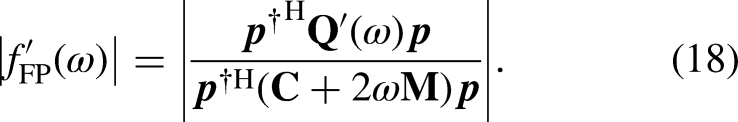
This yields a closed-form expression for the sensitivity of the mapping $f$ as required to apply Banach’s theorem:

$$|f_{\mathrm{FP}}^{\prime }(\omega )|=\left|\frac{{{\mathit{p}}^{†}}^{\mathrm{H}}{\mathbf{Q}}^{\prime }(\omega )\mathit{p}}{{\mathit{p}}^{†\mathrm{H}}(\mathbf{C}+2\omega \mathbf{M})\mathit{p}}\right|.$$

(18)

The mapping sensitivity (18) is generally expected to be non-zero. This implies that, if the fixed-point iteration converges, $|f^{\prime }|<1$ , then it possesses a linear convergence rate – see Eq. (21).

An alternative fixed-point iteration scheme

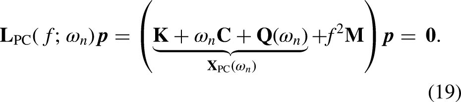
The choice of a fixed-point iteration method is not unique. One of the disadvantages of the solution method proposed in ³ is that it casts the original problem in an eigenvalue problem having doubled dimensions, which is computationally more expensive to solve. Alternatively, one can perform an iteration in the ${\omega }^2$ term of Eq. (3), while the remaining occurrences of the eigenvalues are fixed to ${\omega }_n$ . The square root of the eigenvalues of the resulting (linear) eigenvalue problem are then an approximation of the sought eigenvalues. This choice is convenient since the matrix $\mathsf{M}$ that appears on the r.h.s. of the resulting generalised eigenvalue problem is positive definite, allowing for the use of robust linear eigenvalue solvers. We shall refer to this solution scheme, described in Alg. 2, as Picard iteration. ¹¹ p. 154

Algorithm 2

Picard iteration

1: function ITERATE( ${\omega }_1,{\mathit{p}}_1,{\mathrm{tol}}_{\omega },\mathrm{maxiter},\mathbf{K}\mathbf{,}\mathbf{C}\mathbf{,}\mathbf{M}\mathbf{,}\mathbf{Q}$ )

2:  ${\omega }_0\leftarrow \mathrm{\infty }$

3:  $n\leftarrow 1$

4: while $|{\omega }_n-{\omega }_{n-1}|>{\mathrm{tol}}_{\omega }$ and $n<\mathrm{maxiter}$ do

5:    $\mathbf{X}\leftarrow \mathbf{K}+{\omega }_n\mathbf{C}+\mathbf{Q}({\omega }_n)$

6:    ${\omega }_{n+1},{\mathit{p}}_{n+1}\leftarrow \mathrm{EIGS}\left(-\mathbf{X},\mathbf{M},{\omega }_n,{\mathit{p}}_n\right)$

7:    ${\omega }_{n+1}\leftarrow \sqrt{{\omega }_{n+1}}$

8:    $n\leftarrow n+1$

9: end while

10: return ${\omega }_n,{\mathit{p}}_n,n$

11: end function

The Picard iteration defines the mapping $f$ given by

$${\mathsf{L}}_{\mathrm{PC}}(f;{\omega }_n)\mathit{p}=(\underset{{\mathsf{X}}_{\mathrm{PC}}({\omega }_n)}{\underbrace{\mathbf{K}+{\omega }_n\mathbf{C}+\mathbf{Q}({\omega }_n)}}+f^2\mathbf{M})\mathit{p}=\mathbf{0}.$$

(19)

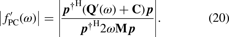
By invoking the associated adjoint eigenvalue problem, and by using the adjoint sensitivity Eq. (16), one can show that the sensitivity of the Picard iteration reads

$$|f_{\mathrm{PC}}^{\prime }(\omega )|=\left|\frac{{{\mathit{p}}^{†}}^{\mathrm{H}}({\mathbf{Q}}^{\prime }(\omega )+\mathbf{C})\mathit{p}}{{{\mathit{p}}^{†}}^{\mathrm{H}}2\omega \mathbf{M}\mathit{p}}\right|.$$

(20)

Notably, the only difference with respect to the sensitivity of the fixed-point iteration proposed by ³ , Eq. (17), is that the matrix $\mathsf{C}$ is moved to the numerator. However, for the simple boundary conditions considered in this study, one finds that the matrix $\mathbf{C}$ has non-zero elements only at the open-end boundary, where both $\mathit{p}$ and ${\mathit{p}}^{†}$ vanish, so that the contribution of the term ${\mathit{p}}^{{†}^{\mathrm{H}}}\mathbf{C}\mathit{p}$ vanishes.

This is a general result. When considering non-trivial boundary conditions, the convergence properties of the two proposed fixed-point solution methods are going to differ, and one cannot draw general conclusions on which method will be able to identify more eigenvalues a priori. On the other hand, for trivial (open and/or closed) boundary conditions one can show that ${\mathit{p}}^{{†}^{\mathrm{H}}}\mathbf{C}\mathit{p}=0$ . Therefore, when considering geometries with simple open or closed boundary conditions, the Picard iteration method should be preferred as a fixed-point iteration scheme since (i) it is computationally cheaper and (ii) has the same contraction properties at the eigenvalues.

Convergence properties of fixed-point iterative methods

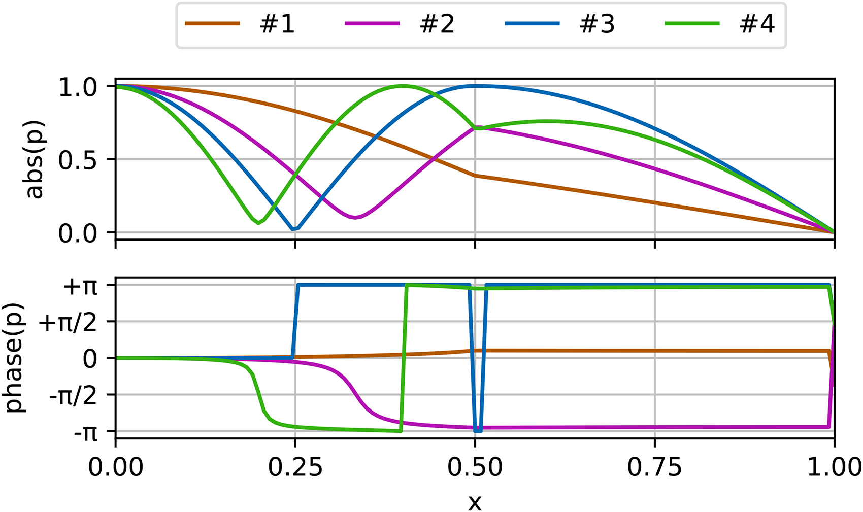
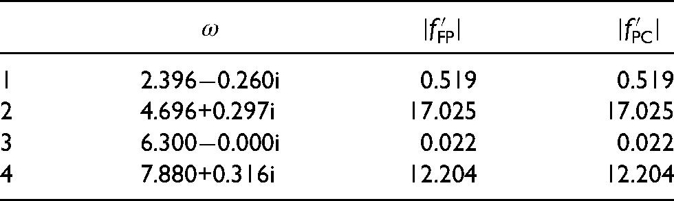
Table 2 highlights the contraction properties of the discussed fixed-point algorithm for the four eigenvalues of interest that the problem has when discretized using an equidistant linear finite elements mesh with 127 degrees of freedom. These eigenvalues have been calculated using a higher-order iterative method, described in the next section. This is because, as we will now show, fixed-point methods fail in identifying some eigenvalues. The modeshapes associated with the four eigenvalues are shown in Figure 1.

Figure 1.

Modeshapes of the four eigenvalues in the considered portion of the complex plane. The colors orange, purple, blue and green indicate, respectively, the thermoacoustic modes number 1, 2, 3 and 4, as listed in Table 2. Modes 1 and 3 are of acoustic origin, 2 and 4 of ITA origin (see Table 1).

Table 2.

Eigenvalues identified by means of finite elements and values of the contracting operator $|f^{\prime }|$ . Only the eigenvalues for which $|f^{\prime }|<1$ can be identified, provided that an accurate initial guess is known.

	$\omega$	$|f_{\mathrm{FP}}^{\prime }|$	$|f_{\mathrm{PC}}^{\prime }|$
1	2.396 $-$ 0.260 $\mathrm{i}$	0.519	0.519
2	4.696+0.297 $\mathrm{i}$	17.025	17.025
3	6.300 $-$ 0.000 $\mathrm{i}$	0.022	0.022
4	7.880+0.316 $\mathrm{i}$	12.204	12.204

The sensitivities that the mapping $f$ takes at these solutions in Table 2 are then evaluated according to Eq. (18). By comparison with Table 1 one finds that $|f^{\prime }|$ is less than one for thermoacoustic modes of acoustic origin, whereas it is greater than one for modes of ITA origin. This implies that modes of ITA origin cannot be identified with this iterative scheme. Indeed, even if a good initial estimate is known for those, since $|f^{\prime }|>1$ the iterative algorithm will repel the initial guess from the actual solution. This fact might be partly responsible for the late discovery of modes of ITA origin in thermoacoustics, in particular for annular combustion chambers,^21,24 for which larger nonlinear eigenvalue problems need to be solved.

Although a formal proof is not available, the difficulties that the fixed-point iterations have in converging towards some ITA modes can be intuitively explained by the following argument. The matrix in the numerator of (18) is proportional to the flame delay, $\exp (-\mathrm{i}\omega \tau )$ . Modes of ITA origin tend to have largely negative growth rates, $\mathrm{\Im }[\omega ]\gg 0$ , implying that $|\exp (-\mathrm{i}\omega \tau )|\gg 1$ . Additionally, the eigenvectors of modes of ITA origin (and their adjoint) have a strong magnitude at the flame – see Figure 1 – exactly the zone in which the flame response $\mathsf{Q}$ is large, due to a strong gradient in the pressure modeshapes at the reference position. In combination, these two effects yield a large value of the term ${{\mathit{p}}^{†}}^{\mathrm{H}}{\mathbf{Q}}^{\prime }(\omega )\mathit{p}$ , appearing in the numerator of (18). Thus, $|f^{\prime }|\gg 1$ can be expected for ITA modes. This statement is not expected to hold generally, but only serves to explain the different convergence behaviours of modes of intrinsic and acoustic origin for this specific case. Indeed, per Eq. (18), a different choice of boundary conditions – via complex-valued impedances in $\mathsf{C}$ or more terms associated with different boundaries – can decrease the value of $|f^{\prime }|$ below unity. When this is the case, then also intrinsic modes could be computed with a fixed-point iteration.

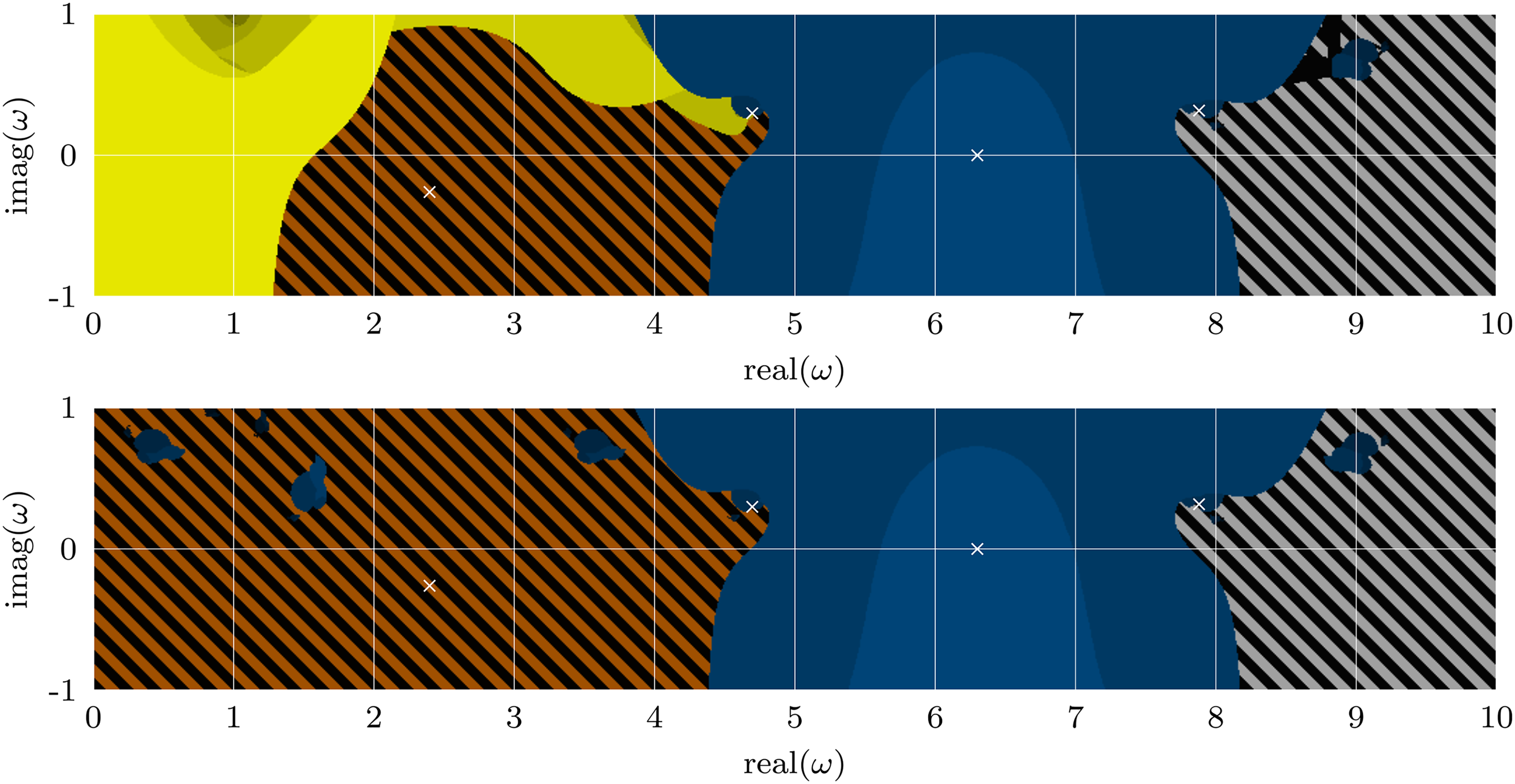
To demonstrate that the fixed-point iterations cannot identify modes for which $|f^{\prime }|>1$ , we perform a large number of brute-force calculations in the complex plane. We initialize the fixed-point algorithm with initial guesses ${\omega }_1$ in the region $\mathcal{S}$ defined in (8) sampled on a uniform $1001\times 201$ grid. The eigenvectors for the Krylov-subspace methods were initialized with the ${\mathit{p}}_1=[1,1,\dots ,1{]}^{\mathrm{T}}$ . We stop the algorithm when a tolerance ${\mathrm{tol}}_{\omega }\equiv |{\omega }_n-{\omega }_{n-1}|<{10}^{-10}$ is reached – an eigenvalue has converged – or when a maximum number of 16 iterations is exceeded – the algorithm does not converge with this initial condition to the desired tolerance. The results are shown in Fig. 2. The axes indicate the value taken by the initial guess, and the color scheme indicates to which eigenvalue the initial guess has converged and how many steps it took. The actual solutions are highlighted with white markers.

Figure 2.

Convergence and basins of attractions for (top) the fixed-point iteration described in ³ , Alg. 1, and (bottom) the Picard iteration described in this study, Alg. 2. The areas in orange and blue indicate, respectively, the basins of attraction of the thermoacoustic modes #1 and #3, as listed in Table 2. The basin of attraction of mode #1 is hatched with black because, although the algorithm is slowly converging, the convergence rate is very low, and it takes more than 16 iterations to identify the eigenvalue to the prescribed accuracy of ${10}^{-10}$ . Both methods are unable to identify modes number 2 and 4, of ITA origin. The lighter the color, the less steps are needed for convergence. Gray-black hatched surfaces indicate (slow) convergence towards an eigenvalue outside of the considered domain. Yellow indicates convergence to a (spurious) eigenvalue with $\omega =0$ .

Brute-force numerical calculations confirm that the modes of ITA origin, #2 and #4 in Table 1, cannot be found by using fixed-point iterative methods, even for guesses that start very close to the actual solutions. The modes of acoustic origin, instead, can be identified. The portions of the complex plane that, when used as an initial guess, converge to modes #1 and #3, are highlighted in orange and blue, respectively. Notably, convergence of mode #1 always requires a number of iterations much larger than those needed for mode #3 to converge. This is in line with the fact that the sensitivity of mode #1, although less than 1, is an order of magnitude larger than that of mode #3. More quantitatively, when $0<|f^{\prime }|<1$ , in the vicinity of a solution the number of steps $N_s$ needed to improve the accuracy by an order of magnitude can be estimated by $N_s=\lceil 1/{\log }_{10}(1/|f^{\prime }|)\rceil$ . From the values reported in Table 2, this yields $N_s=4$ for mode #1 and $N_s=1$ for mode #3, i.e., the former requires approximately 4 times more iterations than the latter to converge to a predefined tolerance. Within the required 16 iterations limit, the eigenvalue #1 can be identified with a tolerance of ${10}^{-6}$ . A larger number of iterations is needed to converge to the prescribed tolerance ${\mathrm{tol}}_{\omega }={10}^{-10}$ , emphasized by the presence of black stripes in Figure 2. Lastly, in yellow we have highlighted the portion of the complex plane that converges to the $\omega =0$ eigenvalue. This is always a solution of the thermoacoustic weak form (3), but it represents a spurious solution that does not satisfy the boundary conditions, except when all boundaries are acoustically closed. This spurious solution arises from manipulation of the impedance boundary condition equations when deriving the weak form (3). The fixed-point algorithm proposed by ³ and summarised in Alg. 1 strongly promotes convergence towards this spurious eigenvalue because it separates the action of the boundary matrix, $\mathbf{C}$ , from that of the stiffness and flame matrices, $\mathsf{K}$ and $\mathsf{Q}$ , as can be seen in Eq. (10).

Together with the higher dimensions of the linearized eigenvalue problem, the promotion of the convergence towards a spurious eigenvalue is another disadvantage of the method of ³ in contrast to the Picard iteration (19). Nonetheless, the slow convergence of some modes and the non-convergence of other modes for both fixed-point iterations are inherently linked to their linear convergence rate. To overcome this limitations, we will now consider methods with a super-linear convergence rate.

Newton-like iteration methods

A sequence generated from an iterative algorithm is said to have a rate of convergence $m$ if there exists a bound $G>0$ such that

$$|{\omega }_{n+1}-\omega |\le G|{\omega }_n-\omega {|}^m.$$

(21)

When the contraction condition (13) is satisfied, the iterative fixed-point algorithms described so far converge towards the closest eigenvalue at a linear rate, $m=1$ . However, when one has $|f^{\prime }(\omega )|=0$ , the rate of convergence becomes super-linear, with $m>1$ . Importantly, $|f^{\prime }(\omega )|=0$ always satisfies Banach’s condition (13), implying that super-linear converging algorithms are guaranteed to converge to all eigenvalues. Super-linear convergence is a feature of Newton’s method, which is therefore more robust than fixed-point methods (0th order), since it uses gradient information (1st order). Gradient information may be included also in a fixed-point iteration by introducing a relaxation parameter ²⁵ Appenidx C.4. This procedure is however based on finite difference approximations and requires solving two eigenvalue problems at each iteration. A direct application of Newton’s method is preferable.

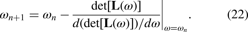
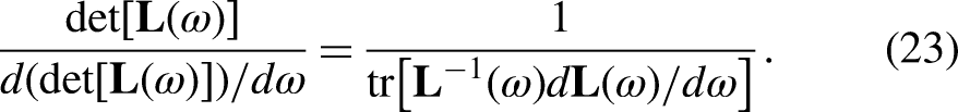
Since the eigenvalues of (3) are found when the determinant of $\mathsf{L}$ vanishes, a direct application of Newton’s method to det $[\mathbf{L}(\omega )]=0$ leads to

$${\omega }_{n+1}={\omega }_n-{\frac{\det [\mathbf{L}(\omega )]}{d(\det [\mathbf{L}(\omega )])/d\omega }|}_{\omega ={\omega }_n}.$$

(22)

Evaluating the determinant is however a demanding and error-prone operation. A determinant-free Newton scheme was suggested in, ²⁶ which exploits Jacobi’s formula

$$\frac{\det [\mathbf{L}(\omega )]}{d(\det [\mathbf{L}(\omega )])/d\omega }=\frac{1}{\mathrm{tr}[{\mathbf{L}}^{-1}(\omega )d\mathbf{L}(\omega )/d\omega ]}.$$

(23)

Although this scheme is more robust than a direct evaluation of the determinant, the evaluation of the inverse of the matrix operator $\mathbf{L}$ becomes prohibitively expensive when $\mathsf{L}$ has hundreds of thousand of degrees of freedom, as is typical in real-world thermoacoustic calculations.

To bypass these issues, in the following section we will discuss how adjoint-based methods allow us to use Newton’s method directly on the NLEVP equations. This will not require the evaluation of determinants nor matrix inverses, and provides more accurate information on the mapping sensitivity than finite difference approximations.

Adjoint-based Newton iteration

By introducing an auxiliary variable $\lambda$ , the NLEVP (2) can be written as

$$\mathbf{L}(\omega )\mathit{p}=\lambda \mathbf{Y}\mathit{p}\mathbf{.}$$

(24)

Equation (24) can be thought of as a generalized eigenvalue problem with eigenvalue $\lambda$ depending on a parameter $\omega$ . From this viewpoint $\lambda$ is an implicitly defined function of $\omega$ , i.e. $\lambda =\lambda (\omega )$ . If the parameter $\omega$ is chosen such that the eigenvalue problem (24) has an eigenvalue $\lambda =0$ , then $\omega$ (and the corresponding eigenvector $\mathit{p}$ ) is a solution of the NLEVP (2). Since the implicitly restarted Arnoldi algorithm is used to solve the sparse eigenvalue problem (24), linear in $\lambda$ , choosing the matrix $\mathbf{Y}$ to be semi-positive definite has significant advantages. Possible choices are $\mathbf{Y}\mathbf{=}\mathbf{I}$ , the identity matrix, or $\mathbf{Y}\mathbf{=}\mathbf{M}$ , the mass matrix. In our analysis the latter will be used, since it naturally arises when discretizing the continuous thermoacoustic operator by means of finite elements. The following discussion on the convergence of the method is however independent from the specific form chosen for $\mathbf{Y}$ .

To find values of $\omega$ for which (24) has a zero eigenvalue in $\lambda$ , we seek the roots of the implicit relation $\lambda =\lambda (\omega )$ . Newton’s iteration on this relation reads

$${\omega }_{n+1}={\omega }_n-\lambda ({\omega }_n)/{\lambda }^{\prime }({\omega }_n)=f({\omega }_n),$$

(25)

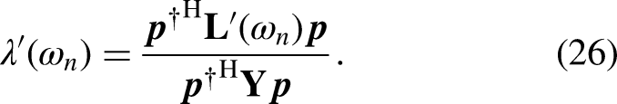
which requires the sensitivity of the eigenvalue with respect to the parameter, ${\lambda }^{\prime }=d\lambda /d\omega$ . This sensitivity can be obtained by means of adjoint methods. Starting from Eq. (24) it can be shown that the sensitivity of a linear eigenvalue problem is^22,23,27

$${\lambda }^{\prime }({\omega }_n)=\frac{{{\mathit{p}}^{†}}^{\mathrm{H}}{\mathbf{L}}^{\prime }({\omega }_n)\mathit{p}}{{{\mathit{p}}^{†}}^{\mathrm{H}}\mathbf{Y}\mathit{p}}.$$

(26)

By using this expression, one can iteratively update the parameter $\omega$ in (25) until an eigenvalue $\lambda =0$ is found.

Algorithm 3

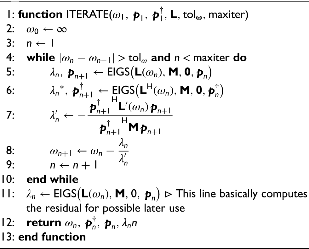
Newton adjoint-based method

1: function ITERATE( ${\omega }_1,{\mathit{p}}_1,{\mathit{p}}_1^{†},\mathbf{L}\mathbf{,}{\mathrm{tol}}_{\omega }\mathbf{,}\mathrm{maxiter}$ )

2:  ${\omega }_0\leftarrow \mathrm{\infty }$

3:  $n\leftarrow 1$

4: while $|{\omega }_n-{\omega }_{n-1}|>{\mathrm{tol}}_{\omega }$ and $n<\mathrm{maxiter}$ do

5:    ${\lambda }_n,{\mathit{p}}_{n+1}\leftarrow \mathrm{EIGS}\left(\mathbf{L}({\omega }_n),\mathbf{M}\mathbf{,}\mathbf{0}\mathbf{,}{\mathit{p}}_n\right)$

6:    ${{\lambda }_n}^{*},{\mathit{p}}_{n+1}^{†}\leftarrow \mathrm{EIGS}\left({\mathbf{L}}^{\mathrm{H}}({\omega }_n),\mathbf{M}\mathbf{,}\mathbf{0}\mathbf{,}{\mathit{p}}_n^{†}\right)$

7:    ${\lambda }_n^{\prime }\leftarrow -\frac{{{\mathit{p}}_{n+1}^{†}}^{\mathrm{H}}{\mathbf{L}}^{\prime }({\omega }_n){\mathit{p}}_{n+1}}{{{\mathit{p}}_{n+1}^{†}}^{\mathrm{H}}\mathbf{M}{\mathit{p}}_{n+1}}$

8:    ${\omega }_{n+1}\leftarrow {\omega }_n-\frac{{\lambda }_n}{{\lambda }_n^{\prime }}$

9:    $n\leftarrow n+1$

10: end while

11:  ${\lambda }_n\leftarrow \mathrm{EIGS}\left(\mathbf{L}({\omega }_n),\mathbf{M},0,{\mathit{p}}_n\right)$ ⊳ This line basically computes the residual for possible later use

12: return ${\omega }_n,{\mathit{p}}_n^{†},{\mathit{p}}_n,{\lambda }_{n}n$

13: end function

The algorithm for the adjoint-based Newton iteration is given in Alg. 3. Note that this method requires solving both the direct and the adjoint problem, which requires a numerical implementation of the adjoint matrix ${\mathbf{L}}^{†}$ . This may cause difficulties in codes which are implemented in a matrix-free fashion, or in which the direct and adjoint discrete equations are derived independently from the continuous equations, and have different discretizations. ³³ In our implementation ^d , the elements of the sparse matrix $\mathbf{L}$ are explicitly stored. Furthermore, since we employ a Bubnov-Galerkin finite elements discretization, the discretization of the continuous adjoint equation is equivalent to the adjoint of the discretized direct equation, and one can show that ${\mathbf{L}}^{†}\mathbf{=}{\mathbf{L}}^{\mathrm{H}}$ . ³⁴ As always for mappings obtained from Newton’s method, the mapping defined by (25) has super-linear convergence, i.e. $f^{\prime }=0$ . This guarantees that all thermoacosutic eigenvalues are attractors for this iteration method, and, provided sufficiently good guesses are provided, they can always be identified. This is formally shown in the Appendix.

Householder’s methods

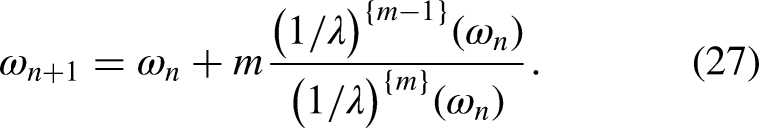
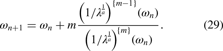
Newton’s method can be generalized by considering higher-order expansions of the relation $\lambda =\lambda (\omega )$ . The resulting class of iterative root-finding methods are known as Householder’s methods. ³⁰ At an arbitrary order $m>0$ the iterative Householder step reads

$${\omega }_{n+1}={\omega }_n+m\frac{{(1/\lambda )}^{\{m-1\}}({\omega }_n)}{{(1/\lambda )}^{\{m\}}({\omega }_n)}.$$

(27)

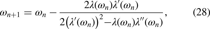
At first order ( $m=1$ ), Eq. (27) corresponds to the Newton iteration (25). At second order ( $m=2$ ) one obtains

$${\omega }_{n+1}={\omega }_n-\frac{2\lambda ({\omega }_n){\lambda }^{\mathrm{\prime }}({\omega }_n)}{2{({\lambda }^{\mathrm{\prime }}({\omega }_n))}^2-\lambda ({\omega }_n){\lambda }^{\mathrm{″}}({\omega }_n)},$$

(28)

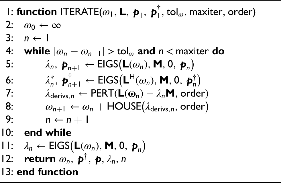
which is also known as Halley’s method. ²⁹ In order to apply higher-order Householder’s methods, the evaluation of high-order eigenvalue sensitivities ${\lambda }^{\{m\}}$ is required. Once again, adjoint-based theory can be exploited in this regard. By using perturbation theory, explicit formulas for the calculation of arbitrarily high-order sensitivity have been derived in, ³⁶ to which we refer the interested reader. For the purpose of this study, we shall assume that a function pert that computes arbitrarily high-order sensitivities is available. With this at hand, the pseudocode for the Householder iterative method is given in Alg. 4, in which the function house computes the Householder update to ${\omega }_n$ at the desired order, according to Eq. (27).

Algorithm 4

Householder’s method

1: function ITERATE( ${\omega }_1,\mathbf{L},{\mathit{p}}_1,{\mathit{p}}_1^{†},{\mathrm{tol}}_{\omega },\mathrm{maxiter},\mathrm{order}$ )

2:  ${\omega }_0\leftarrow \mathrm{\infty }$

3:  $n\leftarrow 1$

4: while $|{\omega }_n-{\omega }_{n-1}|>{\mathrm{tol}}_{\omega }$ and $n<\mathrm{maxiter}$ do

5:    ${\lambda }_n,{\mathit{p}}_{n+1}\leftarrow \mathrm{EIGS}\left(\mathbf{L}({\omega }_n),\mathbf{M},0,{\mathit{p}}_n\right)$

6:    ${\lambda }_n^{*},{\mathit{p}}_{n+1}^{†}\leftarrow \mathrm{EIGS}\left({\mathbf{L}}^{\mathrm{H}}({\omega }_n),\mathbf{M},0,{\mathit{p}}_n^{†}\right)$

7:    ${\lambda }_{\mathrm{derivs},n}\leftarrow \mathrm{PERT}\left(\mathbf{L}({\omega }_n)-{\lambda }_n\mathbf{M}\mathbf{,}\mathrm{order}\right)$

8:    ${\omega }_{n+1}\leftarrow {\omega }_n+\mathrm{HOUSE}({\lambda }_{\mathrm{derivs},n},\mathrm{order})$

9:    $n\leftarrow n+1$

10: end while

11:  ${\lambda }_n\leftarrow \mathrm{EIGS}\left(\mathbf{L}({\omega }_n),\mathbf{M},0,{\mathit{p}}_n\right)$

12: return ${\omega }_n,{\mathit{p}}^{†},\mathit{p},{\lambda }_n,n$

13: end function

Convergence properties of Householder’s methods

By construction, all Houselder’s methods have $f^{\prime }=0$ at the fixed points, implying that all eigenvalues are attractors and have a non-empty basin of attraction. When considering simple roots, the $m$ th order Householder’s method has a convergence rate of $m+1$ , meaning that a lower number of iterations in generally required to identify a solution. Yet, these methods are generally not applied to scalar equations because the increase in function evaluations per iteration outweighs the improved convergence rate when the order is increased. This limitation however does not straightforwardly apply to large eigenvalue problems. This is because one needs to weight the computational effort needed for the solution of a linear eigenvalue problem at each step – ruled by the dimension of the problem only – against the one needed to perform all the matrix-vector products needed – which depends on the problem size, but also significantly increases at each perturbation order. ³⁶ Thus, for adjoint-based perturbation theory applied on large matrices, computational optimality is ruled by a non-trivial trade-off between the number of iterations needed to converge and the cost of the perturbation method at the chosen order. Numerical experiments have shown (details not reported here) that the Householder’s method of order 3 has, on average, optimal performances (minimum time and memory used) for eigenvalue problems that have a few thousands degrees of freedom.

Degenerate eigenvalues

Special care needs to be taken if the eigenvalue searched for is a multiple root of the characteristic function of $\mathbf{L}$ , i.e., if the eigenvalue is degenerate. For degenerate semi-simple eigenvalues perturbation theory can still be used to compute the necessary derivatives.^32,38 To retain the high convergence rate of Householder’s methods, the scheme must be applied to the $a$ th root of $\lambda$ , where that $a$ is the algebraic multiplicity of the eigenvalue. The $m$ th order expansion reads

$${\omega }_{n+1}={\omega }_n+m\frac{{(1/{\lambda }^{\frac{1}{a}})}^{\{m-1\}}({\omega }_n)}{{\left({1/\lambda }^{\frac{1}{a}}\right)}^{\{m\}}({\omega }_n)}.$$

(29)

This however requires a priori knowledge on the multiplicity of an eigenvalue. In thermoacoustic applications, degeneracies with multiplicity 2 are typically induced by symmetries of the system ³⁷ and can be often predicted with intuition and/or the use of symmetry breaking criteria. ³⁵ In most cases, multiplicities can be removed from the problem by a proper symmetry reduction scheme, such as reduction to Bloch-periodic unit cells. ¹⁷ Lastly, in case of defective eigenvalues, the adjoint-based schemes presented here cannot be applied, because defective eigenvalues are not analytic in their parameters. However, defective eigenvalues can only appear as isolated points in the parametrized spectrum of $\mathbf{L}$ ³¹ and are, thus, not considered generic.

Convergence examples

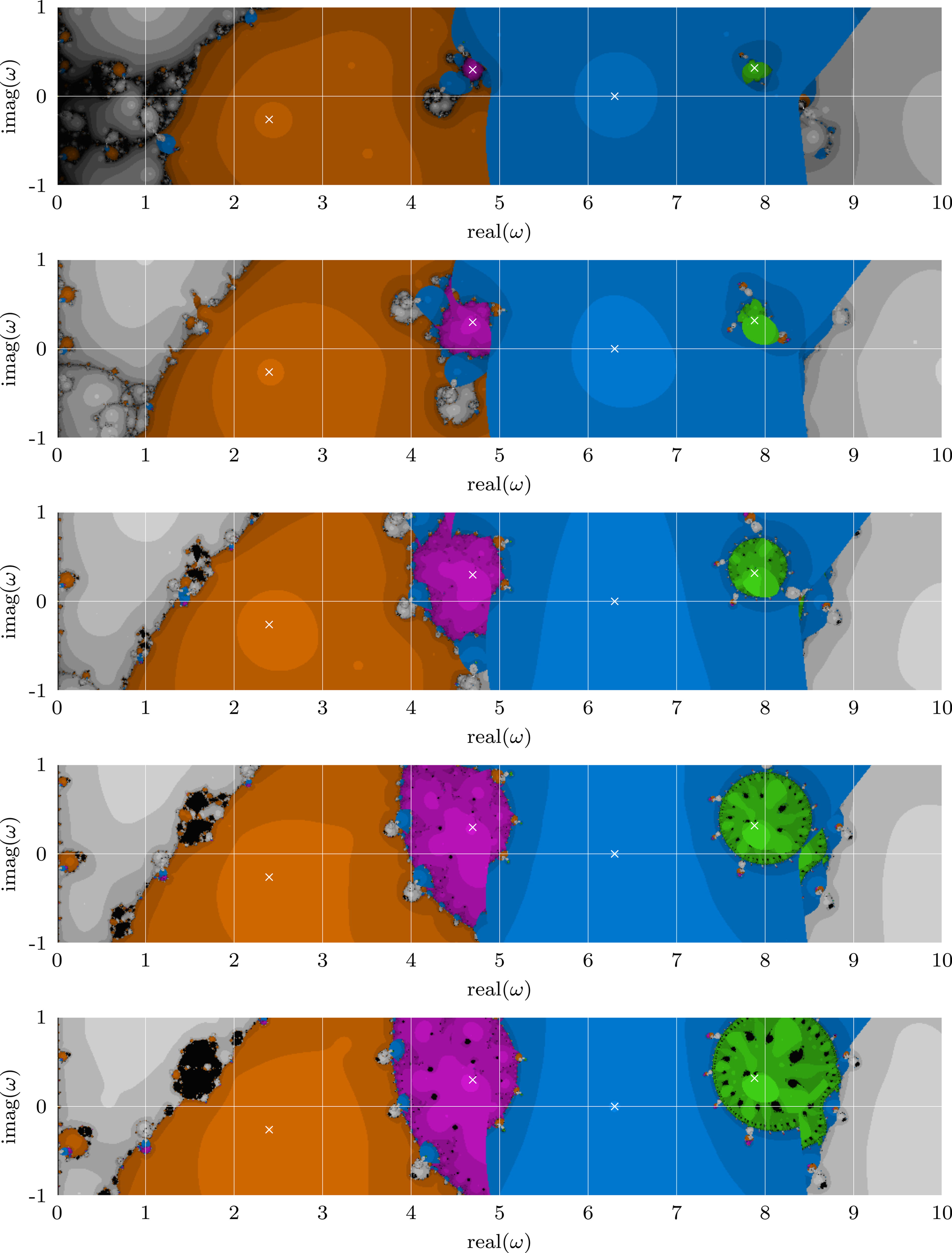
Figure 3 shows the eigenvalue convergence maps when using Householder’s methods from first order (top) to fifth order (bottom). The tolerance for convergence is set to ${\mathrm{tol}}_{\omega }={10}^{-10}$ for all cases. The convergence properties have significantly improved compared to those of the fixed-point methods shown in Figure 2. Indeed, for all considered orders of the Houselder’s method, all the four thermoacoustic eigenvalues in the considered portion of the complex plane can be found. In fact, as predicted by Banach’s theorem for this mapping each mode possesses a non-empty basin of attraction in its vicinity – recall that $f^{\prime }=0$ . Furthermore, the higher the order of the considered Householder iteration, the fewer iteration steps are generally needed to converge to the desired accuracy, as can be seen from the fact that the higher is the perturbation order, the brighter is its figure. This does not necessarily mean a faster convergence time, but it demonstrates the increase in convergence rate, Eq. (21), with an increase in the order of the method $m$ . Another notable feature of the Householder’s methods is that the size of the basins of attraction of the ITA modes (purple and green) grows when the order of the method is increased. This implies that, when using a (say) fourth order Householder scheme (fourth row in Figure 3), a coarse grid of initial guesses is sufficient to identify all the eigenvalues of interest. On the other hand for the Newton method (top row in Figure 3), although the basins of attraction of modes of ITA origin are non-empty, they have a small size. A finer mesh of initial guesses is therefore required if the eigenvalues are randomly searched. Higher-order Householder’s scheme suffer, however, from the existence of larger portions of the complex plane within which the method does not converge to any eigenvalues (in black).

Figure 3.

Convergence and basins of attractions for the Householder’s methods from first order (top, also known as Newton’s method) to fifth order (bottom). The areas in orange, purple, blue and green indicate, respectively, convergence to the thermoacoustic modes number 1, 2, 3 and 4, as listed in Table 2. Modes 1 and 3 are of acoustic origin, 2 and 4 of ITA origin. The lighter the color, the less steps are needed for convergence. Gray indicates convergence to an eigenvalue outside of the considered domain. Black indicates that the algorithm does not converge with these initial conditions.

All these considerations suggest that a third order Householder scheme is on average the optimal choice, as it provides both faster computational times and possess good convergence properties.

To conclude, we remark that the convergence maps show fractal patterns at the boundaries between different basins of attraction. The fractal nature of the boundaries of attraction (sometimes referred to as Julia sets) is a known feature of Newton-like iteration maps already when applied to scalar equations. ²⁸ However, we note how some of the boundaries in Figure 3 are non-fractal. This can be attributed to the fact that we apply Newton/Householder’s methods to eigenvalue problems. Our adjoint-based algorithms require the identification of the smallest eigenvalue of a linear eigenvalues problem to the initial guess (see Alg. 3 and 4). This choice becomes ambiguous when the closest eigenvalue of the linear eigenvalue problem (24) becomes degenerate. This is what happens at non-fractal boundaries, and the clear-cut between convergence to two different eigenvalues when using very close guesses is explained by the fact that our solution method suddenly tracks a different eigenvalue branch of the linear eigenvalue problem.

Conclusions

In this study, we have investigated the convergence properties of the most common methods used to identify eigenvalues in thermoacoustic systems by means of iterative methods. By exploiting adjoint-based sensitivity, we have derived explicit equations that can be used to assess the contraction properties of various algorithms in the vicinity of eigenvalues. Thanks to Banach’s fixed-point theorem, this information is sufficient to know if a given algorithm can or cannot converge to an eigenvalue.

For fixed-point iterations, which are commonly employed in thermoacoustics, we found that not all eigenvalues are attractors. In particular, numerical calculations on a Rijke tube system showed that thermoacoustic modes of ITA origin are repellors. This implies that these eigenvalues can never be identified by fixed-point algorithms, regardless on the accuracy of the initial guess. This may be linked to the late discovery of ITA modes by the thermoacoustic community.

We then discussed how Newton-like iterative methods should always be preferred to fixed-point iterations. This is because they are always guaranteed to converge to all eigenvalues, provided that sufficiently good initial guesses are provided. The most straightforward use of Newton’s method to eigenvalue problems, however, is inefficient, as it requires the evaluation of matrix determinants or inverses, which becomes prohibitively expensive for large matrices. To overcome this issue, we have introduced a set of adjoint-based methods, known as Householder’s methods, which make use of high-order perturbation expansions. We have discussed both the computational efficiency of the algorithms and the dimensions of the basins of attractions of the eigenvalues for these methods up to 5th order. By combining formal results and numerical evidence, we conclude that a third order Householder’s method is, among the methods discussed in this study, the optimal choice for identifying eigenvalues of thermoacoustic systems.

Our results highlight the importance on the choice of the solution methods for thermoacoustic eigenvalue problems. In particular, fixed-point iterations should be always avoided since they do not guarantee the identification of all the eigenvalues, and failure in identifying potentially unstable thermoacoustic modes at the design stage can have very expensive side-effects.