Some new chiral and perturbed chiral solitary waves in quantum Hall effect

Abstract

In this article, we present a new form of solutions to the Chiral/perturbed Chiral nonlinear Schrödinger equation, using the unified solver method. This solver introduces the closed formula in an explicit way. In each problem, different families of elliptic functions solutions are found under suitable conditions. Moreover, some cases of hyperbolic solutions are obtained. The acquired solutions may be applicable for explaining various complex phenomena in the quantum Hall effect. The presented study displays that the proposed solver is simple, powerful and sturdy. For more details about the physical dynamical representation of the presented solutions, we introduce some graphs of some selected solutions using Matlab software. Finally, the presented solver can be used to solve many other models in real life problems.

Introduction

Investigation of optical solutions has distinctly acquired momentum in the field of the solitary waves.^1–5 In dielectric fibers, the dynamic balance between the optical Kerr effect and dispersion generates an optical solution. Indeed, solutions have acquired much attention because of their robust nature and powerful applications in all long-distance and optical communications.^6–12 Due to the nonlinear Schrödinger equation’s (NLSE’s) rich physical features, optical solutions, namely, complex and hyperbolic solitons, are now the most interesting fields of nonlinear wave propagation in plasma of fluids, electromagnetic wave propagation, deep water, quantum mechanics, superconductivity, electromagnetic wave propagation, nuclear physics, and magneto-static spin waves optical fibers communications.^13–21 Various physicists and mathematicians proposed and developed some standing wave stabilities for NLSEs and related equations such as perturbed, Hartree, Choquard, and its fractional form equations.^22–27

The concept of chiral solitons represents a crucial role in the developments of quantum mechanics, specifically, in the field of quantum Hall effect (QHE) and biological sciences in the context of neurosciences, where the appearance of chiral solitons is known to appear. In 1980, Klaus von Klitzing investigated the relation between the QHE and fundamental physical constants for which he received a Nobel Prize in 1985. The chiral NLSE (CNLSE) was investigated earlier where both bright and dark soliton solutions were given. ²⁸ The (1+1)-dimensional CNLSE is ²⁸

$$i{q}_t+q_{xx}-i\delta (q^{*}{q}_x-q{q}_x^{*})q=0,i=\sqrt{-1}$$

(1)

where $\delta$ is a nonlinear coupling constant, $q(x,t)$ is a complex function of $x$ and $t$ , and the $q^{*}$ indicates it’s complex conjugate. The first term on the left-hand side denotes the evolution term and the second term denotes the dispersion. Subsequently, in 2004, Bohm potential was presented and various studies were done with new perturbed NLSE (where Bohm potential was taken as the perturbation term, x),^29,30 given by

$$i{q}_t+a{q}_{xx}-ib(q^{*}{q}_x-q{q}_x^{*})q=i\alpha q\frac{\mid q{\mid }_{xx}}{\mid q\mid }$$

(2)

where $a$ denotes the coefficient of dispersion and $b$ denotes a nonlinear coupling constant. On the right-hand side, which is called the perturbation term, the coefficient $\alpha$ is known as Bohm potential. The perturbed CNLSE (PCNLSE) has remarkable applications in the development of quantum mechanics, which give us the main basics of a hidden variable theory. Thus, it is important to find exact solutions of PCNLSE for the development of quantum mechanics. There are various approaches have been applied to extract solutions of the PCNLSE, such as the extended fan sub-equation method, ³¹ extended modified auxiliary equation mapping method, ³² and many other techniques, for example, see.^33–37

Our work is devoted to extracting new solutions for the CNLSE and PCNLSE, using the unified solver method. ³⁸ The main advantage of utilizing this technique is to get different family solutions via free physical parameters. The unified solver method is well-structured, simple, adequate, and efficient It is avoiding challenging and time-consuming computations and offering accurate solutions. Indeed, physicists, engineers, and mathematicians can employ the suggested solver as a box solver. The suggested fundamental technique has a number of benefits, including avoiding challenging and time-consuming computations and offering accurate solutions. The presented solutions will be extremely beneficial in many fields of applied sciences, such as nuclear physics, quantum mechanics, fluid mechanics, plasma physics, nonlinear optics, and nanotechnology. Indeed, the proposed solutions are used to study the adiabatic parameter dynamics. To our knowledge, the proposed solver for resolving the CNLSE and PCNLSE has not been used in any prior research.

This article is arranged as follows. The “Unified solver method” section discusses the presented solver technique. The “Applications” section presents the solutions for the CNLSE and PCNLSE, using the unified solver method. The “Results and discussion” section gives some physical interpretation for the gained results. Finally, some conclusions are reported in the “Conclusions” section.

Unified solver method

Consider the following nonlinear partial differential equation:

$$\mathcal{H}(F,F_x,F_t,F_{xx},F_{xt},F_{tt},\dots )=0$$

(3)

Utilizing the suitable wave transformation:

$$F(x,t)=F(\eta ),\eta =x-\nu t$$

(4)

where $\eta$ is the traveling wave transformation and $\nu$ is the velocity speed of the traveling wave, equation (3) will be converted to the following ODE:

$$\mathcal{H}(F,F^{\prime },F^{″},F^{‴},\dots )=0$$

(5)

Various models in natural sciences presented in form of equation (3) can be converted to the following ODE:

$$\mathrm{\Lambda }{F}^{\mathrm{″}}+\mathrm{\Sigma }{F}^3+\mathrm{\Gamma }F=0$$

(6)

where $\mathrm{\Lambda },\mathrm{\Sigma }$ , and $\mathrm{\Gamma }$ are certain constants depend on the constants of the main problem and the velocity speed of the wave transformations.

In view of the unified solver technique introduced by Abdelrahman and AlKhidhr, ³⁸ the solution of equation (6) was assumed to be given in the form of:

$$F=A_0+A_{1}sn(\eta ,n)+A_{2}cn(\eta ,n)$$

(7)

Deriving equation (7) twice gives

$${\mathrm{F}}^{″}=\frac{{\mathrm{d}}^2\mathrm{F}}{\mathrm{d}{\xi }^2}.$$

(8)

$$\begin{array}{r}\begin{array}{cc}{F}^{\mathrm{″}}=& -A_1(n^2+1)sn(\eta ,n)+2A_1{n}^{2}sn(\eta ,n{)}^3\\ & +2A_2{n}^{2}sn(\eta ,n{)}^{2}cn(\eta ,n)-A_{2}cn(\eta ,n)\end{array}\end{array}$$

(9)

Substituting equations (7) and (9) into equation (6) and comparing the coefficients of $sn(\eta ,n{)}^3$ , $sn(\eta ,n{)}^2\mathit{c}\mathit{n}\mathit{(}\eta \mathit{,}\mathit{n}\mathit{)}$ , $sn(\eta ,n{)}^2$ , $sn(\eta ,n)\mathit{c}\mathit{n}\mathit{(}\eta \mathit{,}\mathit{n}\mathit{)}$ , $sn(\eta ,n)$ , $cn(\eta ,n)$ , $sn(\eta ,n{)}^0$ in both sides of the new equation, gives some algebraic equations. Solving these equations for $A_0,A_1$ , and $B_1$ , yields two main cases:

For $n=0$ and $\mathrm{\Sigma }\ne 0$ (or $\mathrm{\Lambda }=0$ ), there exist a constant solution takes the form:

$$F_0(\eta )=\pm \sqrt{\frac{-\mathrm{\Gamma }}{\mathrm{\Sigma }}}$$

(10)

For $0<n<1$ and $\mathrm{\Sigma }\ne 0$ , we obtain four families of solutions $F_i(\eta );i=1,2,3,4$ depending on the values of $A_1,A_2$ , and $n$ , where $A_0=0$ :

Family I

$$A_1=\pm \sqrt{\frac{2(\mathrm{\Lambda }-\mathrm{\Gamma })}{\mathrm{\Sigma }}},A_2=0,n=\sqrt{\frac{\mathrm{\Gamma }}{\mathrm{\Lambda }}-1}$$

The family of solutions $F_1(\eta )$ takes the form:

$$F_1(\eta )=\pm \sqrt{\frac{2(\mathrm{\Lambda }-\mathrm{\Gamma })}{\mathrm{\Sigma }}}\text{sn}(\eta ,\sqrt{\frac{\mathrm{\Gamma }}{\mathrm{\Lambda }}-1})$$

(11)

where

$$1<\frac{\mathrm{\Gamma }}{\mathrm{\Lambda }}<2$$

(12)

Family II

$$A_2=\pm \sqrt{\frac{\mathrm{\Lambda }-\mathrm{\Gamma }}{\mathrm{\Sigma }}},n=\sqrt{\frac{1}{2}(1-\frac{\mathrm{\Gamma }}{\mathrm{\Lambda }})}$$

The form of the solutions $F_2(\eta )$ is given by:

$$F_2(\eta )=\pm \sqrt{\frac{\mathrm{\Lambda }-\mathrm{\Gamma }}{\mathrm{\Sigma }}}\text{cn}(\eta ,\sqrt{\frac{1}{2}(1-\frac{\mathrm{\Gamma }}{\mathrm{\Lambda }})})$$

(13)

where

$$0<\frac{\mathrm{\Gamma }}{\mathrm{\Lambda }}<2$$

(14)

Family III

$$A_1=\pm \sqrt{\frac{\mathrm{\Gamma }-\mathrm{\Lambda }}{\mathrm{\Sigma }}},A_2=-\sqrt{\frac{\mathrm{\Lambda }-\mathrm{\Gamma }}{\mathrm{\Sigma }}},n=\sqrt{2(1-\frac{\mathrm{\Gamma }}{\mathrm{\Lambda }})}$$

The family of solutions $F_3(\eta )$ takes the form:

$$F_3(\eta )=\pm \sqrt{\frac{\mathrm{\Gamma }-\mathrm{\Lambda }}{\mathrm{\Sigma }}}\text{sn}(\eta ,\sqrt{2(1-\frac{\mathrm{\Gamma }}{\mathrm{\Lambda }})}-\sqrt{\frac{\mathrm{\Lambda }-\mathrm{\Gamma }}{\mathrm{\Sigma }}}\text{cn}(\eta ,\sqrt{2(1-\frac{\mathrm{\Gamma }}{\mathrm{\Lambda }})}$$

(15)

where

$$\frac{1}{2}<\frac{\mathrm{\Gamma }}{\mathrm{\Lambda }}<1$$

(16)

Family IV

$$A_1=\pm \sqrt{\frac{\mathrm{\Gamma }-\mathrm{\Lambda }}{\mathrm{\Sigma }}},A_2=\sqrt{\frac{\mathrm{\Lambda }-\mathrm{\Gamma }}{\mathrm{\Sigma }}},n=\sqrt{2(1-\frac{\mathrm{\Gamma }}{\mathrm{\Lambda }}}$$

The fourth family of solutions $F_4(\eta )$ is

$$F_4(\eta )=\pm \sqrt{\frac{\mathrm{\Gamma }-\mathrm{\Lambda }}{\mathrm{\Sigma }}}\text{sn}(\eta ,\sqrt{2(1-\frac{\mathrm{\Gamma }}{\mathrm{\Lambda }})})+\sqrt{\frac{\mathrm{\Lambda }-\mathrm{\Gamma }}{\mathrm{\Sigma }}}\text{cn}(\eta ,\sqrt{2(1-\frac{\mathrm{\Gamma }}{\mathrm{\Lambda }})})$$

(17)

where

$$\frac{1}{2}<\frac{\mathrm{\Gamma }}{\mathrm{\Lambda }}<1.$$

(18)

From the above conditions, we find that there exist:

only one family of solutions $F_2(\eta )$ under the condition $0<\frac{\mathrm{\Gamma }}{\mathrm{\Lambda }}<\frac{1}{2}$ ,

two families of solutions $F_1(\eta )$ and $F_2(\eta )$ under the condition $1<\frac{\mathrm{\Gamma }}{\mathrm{\Lambda }}<2$ ,

three families of solutions $F_j(\eta ),j=2,3,4$ under the condition $\frac{1}{2}<\frac{\mathrm{\Gamma }}{\mathrm{\Lambda }}<1$ .

Hyperbolic functions solutions

From the previous families of elliptic functions solutions, we get the hyperbolic functions solutions, which can appear for certain values of $\frac{\mathrm{\Gamma }}{\mathrm{\Lambda }}$ corresponding to $n=1$ in the following sense:

For $\mathrm{\Gamma }=2\mathrm{\Lambda }$ , equation (11) transforms to

$$F_1(\eta )=\pm \sqrt{\frac{-2\mathrm{\Lambda }}{\mathrm{\Sigma }}}\tanh (\eta )$$

(19)

For $\mathrm{\Gamma }=-\mathrm{\Lambda }$ , equation (13) turns into

$$F_2(\eta )=\pm \sqrt{\frac{2\mathrm{\Lambda }}{\mathrm{\Sigma }}}\text{sech}(\eta )$$

(20)

For $\mathrm{\Gamma }=\mathrm{\Lambda }/2$ , equations (15) and (17) become

$$F_3(\eta )=\pm \sqrt{\frac{-\mathrm{\Lambda }}{2\mathrm{\Sigma }}}\tanh (\eta )-\sqrt{\frac{\mathrm{\Lambda }}{2\mathrm{\Sigma }}}\text{sech}(\eta )$$

(21)

$$F_4(\eta )=\pm \sqrt{\frac{-\mathrm{\Lambda }}{2\mathrm{\Sigma }}}\tanh (\eta )+\sqrt{\frac{\mathrm{\Lambda }}{2\mathrm{\Sigma }}}\text{sech}(\eta )$$

(22)

respectively.

Applications

We implement the presented solver method, to provide new solutions for CNLSE and PCNLSE.

Solutions of CNLSE

CNLSE was given by the form in equation (1). We first use the following complex wave transformation ²⁸ :

$$q(x,t)=e^{i(kx+wt+h)}Q(\eta ),\eta =c(x+\nu t)$$

(23)

where $k$ , $w$ , $h$ , $c$ , and $\nu$ are real constants. Substituting equation (23) into equation (1) and by taking the real and imaginary parts of the reduced equation we get:

$$c^2{Q}^{″}+2k\delta Q^3-(w+k^2)Q=0$$

(24)

and

$$\nu =-2k$$

(25)

respectively. Thus from equations (23) and (25), we get:

$$\eta =c(x-2kt)$$

(26)

The second-order differential equation (24) has the form of equation (6), where

$$\mathrm{\Lambda }=c^2,\mathrm{\Sigma }=2k\delta ,\mathrm{\Gamma }=-(w+k^2)$$

(27)

Thus the solutions of equation (24) take a similar forms of solutions (10), (11), (13), (15), and (17). The solution of equation (1) corresponding to the constant solution of equation (24) takes the form:

$$q_0(x,t)=\pm \sqrt{\frac{(w+k^2)}{2k\delta }}{e}^{i(kx+wt+h)}$$

(28)

For $0<n<1$ , the four families of solutions of equation (1) can be written in the form:

Family I

The first family of solutions takes the form:

$$q_1(x,t)=\pm n_1\sqrt{\frac{-c^2}{k\delta }}{e}^{i(kx+wt+h)}\text{sn}(c(x-2kt),n_1),n_1=\sqrt{-\frac{(w+k^2+c^2)}{c^2}}$$

(29)

where

$$-(k^2+c^2)>w>-(k^2+2c^2)$$

(30)

Family II

The second family of solutions is given in the form:

$$q_2(x,t)=\pm n_2\sqrt{\frac{c^2}{k\delta }}{e}^{i(kx+wt+h)}\text{cn}(c(x-2kt),n_2),n_2=\sqrt{\frac{1}{2c^2}(w+c^2+k^2)}$$

(31)

where

$$-k^2+c^2>w>-(k^2+c^2)$$

(32)

Family III

The third family of solutions can be given as:

$$q_3(x,t)=n_3\sqrt{\frac{c^2}{4k\delta }}[\text{cn}(c(x-2kt),n_3)\pm i\text{sn}(c(x-2kt),n_3)]e^{i(kx+wt+h)},n_3=\sqrt{\frac{2(w+c^2+k^2)}{c^2}}$$

(33)

where

$$-(k^2+\frac{c^2}{2})>w>-(k^2+c^2)$$

(34)

Family IV

For the same value of $n_3$ given in equation (33) and under the same condition (34), we get the fourth family of solutions written as follows:

$$q_4(x,t)=n_3\sqrt{\frac{c^2}{4k\delta }}[\pm i\text{sn}(c(x-2kt),n_3)-\text{cn}(c(x-2kt),n_3)]e^{i(kx+wt+h)}$$

(35)

From the conditions (30), (32), and (34), we find that:

For $-(k^2+c^2)>w>-(k^2+2c^2)$ , there exist only one family of solutions $q_1(x,t)$ .

For $-k^2+c^2>w>-(k^2+\frac{c^2}{2})$ , there exist two families of solutions $q_1(x,t)$ and $q_2(x,t)$ .

For $-(k^2+\frac{c^2}{2})>w>-(k^2+c^2)$ , there exist three families of solutions $q_i(x,t);i=2,3,4$ .

Hyperbolic functions solutions

The hyperbolic functions solutions can appear for specific values of $w$ as follows:

For $w=-(k^2+2c^2)$ equation (29) is transformed to

$$q_1(x,t)=\pm \sqrt{\frac{-c^2}{k\delta }}{e}^{i(kx-(k^2+2c^2)t+h)}\text{tanh}(c(x-2kt))$$

(36)

For $w=-(k^2-c^2)$ , equation (31) turns into

$$q_2(x,t)=\pm \sqrt{\frac{c^2}{k\delta }}{e}^{i(kx-(k^2-c^2)t+h)}\text{sech}(c(x-2kt))$$

(37)

For $w=-(k^2+\frac{c^2}{2})$ , equations (33) and (35) become

$$q_3(x,t)=\sqrt{\frac{-c^2}{4k\delta }}[\pm \tanh (c(x-2kt))-i\text{sech}(c(x-2kt))]e^{i(kx-(k^2+\frac{c^2}{2})t+h)}$$

(38)

and

$$q_4(x,t)=\sqrt{\frac{-c^2}{4k\delta }}[\pm \tanh (c(x-2kt))+i\text{sech}(c(x-2kt))]e^{i(kx-(k^2+\frac{c^2}{2})t+h)}$$

(39)

respectively.

Solutions of the new PCNLSE

The equation of the new PCNLSE is given in equation (2). For this equation the complex wave transformation takes the form:

$$q(x,t)=e^{i(-kx+wt+\theta )}Q(\zeta ),\zeta =x+vt$$

(40)

where $k$ is the soliton wavenumber, $w$ is the frequency of the solitons, $\theta$ is the phase constant, and $v$ is the wave speed.

Substituting from equation (40) into equation (2) and considering the real and imaginary parts separately, gives

$$(v-2ka)Q^{\mathrm{\prime }}(\zeta )-\alpha Q^{\mathrm{″}}(\zeta )=0$$

(41)

$$\mathrm{\Lambda }{Q}^{\mathrm{″}}(\zeta )+\mathrm{\Sigma }{Q}^3(\zeta )+\mathrm{\Gamma }Q(\zeta )=0$$

(42)

where $\mathrm{\Lambda }=a,\mathrm{\Sigma }=-2kb,\mathrm{\Gamma }=-(w+k^{2}a)$ .

The solutions of equation (42) can be obtained by applying the solver demonstrated in the “Unified solver method” section. The form of the solutions is similar to those given above.

For the solutions of equation (2), there are two main cases to discuss:

For $m=0$ & $bk\ne 0$ (or $a=0$ ), there exist a solution given in the form:

$$q_0(x,t)=\pm \sqrt{\frac{-w}{2kb}}{e}^{i(-kx+wt+\theta )}$$

(43)

For $0<m<1$ & $bk\ne 0$ , and by applying the solver demonstrated in the “Unified solver method” section to equation (42), there are four families of solutions presented as follows:

Family I

The formula of the first family of solutions is given by:

$$q_1(x,t)=\pm m_1^{*}\sqrt{\frac{a}{kb}}\text{sn}(x+vt,m_1^{*})e^{i(-kx+wt+\theta )},m_1^{*}=\sqrt{\frac{-(w+k^{2}a)}{a}-1}$$

(44)

where

$$-(k^2+2)<\frac{w}{a}<-(k^2+1)$$

(45)

Family II

The second family of solutions takes the form:

$$q_2(x,t)=\pm m_2^{*}\sqrt{\frac{-a}{kb}}\text{cn}(x+vt,m_2^{*})e^{i(-kx+wt+\theta )},m_2^{*}=\sqrt{\frac{1}{2}(1+\frac{(w+k^{2}a)}{a})}$$

(46)

under the condition

$$-(k^2+2)<\frac{w}{a}<-k^2$$

(47)

Family III

The third family of solutions is given by

$$q_3(x,t)=m_3^{*}\sqrt{\frac{a}{4kb}}[\pm \text{sn}(x+vt,m_3^{*})-i\text{cn}(x+vt,m_3^{*})]e^{i(-kx+wt+\theta )}$$

(48)

$$m_3^{*}=\sqrt{2(1+\frac{(w+k^{2}a)}{a})}$$

(49)

under the condition

$$-(k^2+1)<\frac{w}{a}<-(k^2+\frac{1}{2})$$

(50)

Family IV

Under the same previous condition given by (50) and for the same value of $m_3^{*}$ given by (49) the fourth family of solutions takes the form:

$$q_4(x,t)=m_3^{*}\sqrt{\frac{a}{4kb}}[\pm \text{sn}(x+vt,m_3^{*})+i\text{cn}(x+vt,m_3^{*})]e^{i(-kx+wt+\theta )}$$

(51)

Hyperbolic functions solutions

Hyperbolic functions solutions of equation (42) can be found under certain values for the amount $\frac{w}{a}+k^2$ and are given as follows:

For $\frac{w}{a}=-(k^2+2)$ equation (44) will be transformed to

$$q_1(x,t)=\pm \sqrt{\frac{a}{kb}}\tanh (x+vt)e^{i(-kx+wt+\theta )}$$

(52)

For $\frac{w}{a}=1-k^2$ , equation (46) will take the form

$$q_2(x,t)=\pm \sqrt{\frac{-a}{kb}}\text{sech}(x+vt)e^{i(-kx+wt+\theta )}$$

(53)

For $\frac{w}{a}=-(k^2+\frac{1}{2})$ , equations (48) and (51) become

$$\begin{array}{r}{q}_3(x,t)=\sqrt{\frac{a}{4kb}}(\pm \tanh (x+vt)-i\text{sech}(x+vt))e^{i(-kx+wt+\theta )}\end{array}$$

(54)

$$\begin{array}{r}{q}_4(x,t)\\ & =\sqrt{\frac{a}{4kb}}(\pm \tanh (x+vt)+i\text{sech}(x+vt))e^{i(-kx+wt+\theta )}\end{array}$$

(55)

respectively.

From the conditions (30), (32), and (34) we find that:

For $-k^2>\frac{w}{a}>-(k^2+\frac{1}{2})$ , there exist only one family of solutions $q_2(x,t)$ .

For $-(k^2+1)>\frac{w}{a}>-(k^2+2)$ , there exist two families of solutions $q_1(x,t)$ and $q_2(x,t)$ .

For $-(k^2+\frac{1}{2})>\frac{w}{a}>-(k^2+1)$ , there exist three families of solutions $q_i(x,t);i=2,3,4$ .

Results and discussion

Here, we discuss the presented results to the CNLSE and PCNLSE. It has been reported that some new solutions to these two equations were achieved in the explicit way with free physical parameters via certain constraints. The behavior of the given solutions being solitons, blow up, rough, periodic, explosive, dissipative, etc., depends on the values of the physical parameters in the coefficients of the CNLSE and PCNLSE. For example, the attitude of profile picture of the wave varies from compressive to rarefactive at critical points and stability regions varies in unstable regions at certain critical values (wavenumber).^39,22

The topic of chiral solitons solutions is so important in the developments of QHE, where chiral excitations are known to appear.^40,41 The entire computer industry is built on quantum mechanics. The laser operation is largely based on the quantum mechanics. Moreover, the presented solutions will be quite beneficial in the areas of biological molecules, superfluid, fiber communications, and nuclear physics. For example, the hyperbolic tangent emerges in the calculation of magnetic moment and rapidity of special relativity, and the hyperbolic secant emerges in the profile of a laminar jet. ⁴²

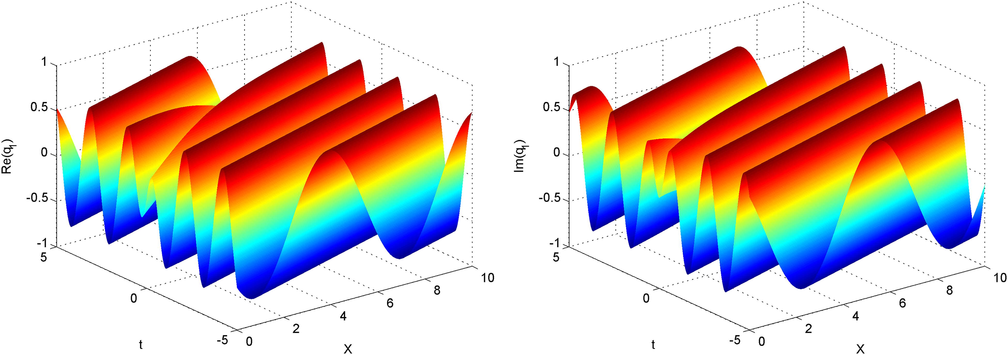
We present some graphs for some selected solutions in order to show the dynamical behavior of these solutions. Figures 1 to 8 depicted these behaviors for certain values of physical parameters. Namely, Figures 1 and 2 depicted the periodic wave of solutions (28) and (36). Figure 3 depicts the envelopes waves for solution (37). Figures 4 to 6 depicted the periodic wave of solutions (38), (43), and (52). Figure 7 depicts the envelopes waves for solution (53). Figure 8 depicts the periodic wave of solution (54). Figures 9 and 10 demonstrate the influence of the parameters on structure, amplitude, phase shift, and bandwidth.

Figure 1.

The surface plot for real and imaginary parts of $q_0(x,t)$ in (28) with the variables $x,t$ , and $k=2$ , $\delta =2$ , $w=1$ , $h=0$ .

Figure 2.

The surface plot for real and imaginary parts of $q_1$ in (36) with $x,t$ , and $c=1$ , $k=2$ , $\delta =2$ , $h=0$ .

Figure 3.

The solution $q_2(x,t)$ in (37) at $h=0$ , $c=1$ when $k\delta >0$ with $c=1$ , $k=1$ , $\delta =2$ , $h=0$ , and $k\delta <0$ with $c=1$ , $k=2$ , $\delta =3$ , $h=0$ .

Figure 4.

The solution $q_3(x,t)$ in (38) when $k\delta >0$ with $x,t$ , and $c=1$ , $k=1$ , $\delta =2$ , $h=0$ .

Figure 5.

The solution $q_o(x,t)$ in (43) at $\theta =0$ when $kb>0$ with $k=1$ , $b=2$ $w=1$ , and $kb<0$ with $k=1$ , $b=2$ $w=1$ .

Figure 6.

The solution $q_1(x,t)$ in (52) when $kb>0$ with $k=1$ , $a=1$ , $b=2$ , $\theta =0$ , $\alpha =1$ and when $kb<0$ with $k=-1$ , $b=2$ $w=1$ , $\theta =0$ , $v=3$ .

Figure 7.

The solution $q_2(x,t)$ in (53) when $kb>0$ with $a=1$ , $k=1$ , $b=2$ , $\theta =0$ , $\alpha =1$ , and when $kb<0$ with $a=-1$ , $k=-1$ , $b=2$ $w=1$ , $\theta =0$ , $v=3$ .

Figure 8.

The solution $q_3(x,t)$ in (54) when $kb>0$ with $a=1$ , $k=1$ , $b=2$ , $\theta =0$ , $v=3$ .

Figure 9.

Trajectory of solutions $q_o(x,t)$ , $q_1(x,t)$ , $q_2(x,t)$ , and $q_3(x,t)$ with $k=2$ , $\delta =2$ , $c=1$ , $h=0$ .

Figure 10.

Trajectory of solutions $q_o(x,t)$ , $q_1(x,t)$ , $q_2(x,t)$ , and $q_3(x,t)$ with $a=1$ , $b=2$ , $w=1$ , $c=1$ , $\theta =0$ , $k=1$ , $v=3$ .

Conclusions

In this study, a unified solver method is used in solving the CNLSEs/PCNLSEs. In both equations, four families of traveling wave solutions are found via free physical parameters under certain constraints. These solutions may be applicable in many interesting applications such as fiber communications, biological molecules, computer industry, magnetic materials, and laser operation. Some 2D and 3D graphs were plotted for different values of parameters to illustrate the behavior of some selected solutions. We observed that the used solver technique is a straightforward and robust tool, which gives vital results when applied to other composite nonlinear models. In future work, we will use other analytical methods to get other forms of solutions. Also, we can analyze the bifurcation and chaotic patterns for of perturbed model with full nonlinearity.