Sage Journals: Discover world-class research

Abstract

In this work, we introduce a new regularized logistic model for the supervised classification problem. Current logistic models have become the preferred tools for supervised classification in many situations. They mostly use either L₁ or L₂ regularization of the weight vector of parameters. Here we take a different approach by applying regularization not to the weight vector but to the gradient vector of the function representing the separating hyper-surface. We present the mathematical analysis of the model in its continuous setting and provide experimental evidence to show that the new model is competitive with state of the art models.

Keywords

Supervised learning variational methods regularization

Introduction

In the last decades, many supervised learning methods have been developed and the ideas behind those models, reviewed consistently in literature.^1–5 Among one of the most complete reviews is the one from Singh et al.,¹ which tests many different methods on a single dataset and presents the results as a list of advantages and disadvantages of every tested method establishing their application areas. A different study, but also very complete, is the one from Fernández-Delgado et al. where 179 classifiers were evaluated on 121 datasets.²

It is difficult to take one side and name the best performing supervised learning algorithm since usually this depends on many factors. The work of Kotsiantis et al.³ brings some light in this direction. In this work the authors conducted a comprehensive review of different classification methods. The results showed that Support Vector Machines (SVM) and Neural Networks (NN) performed the best in terms of accuracy, classification speed and tolerance to parity problems. On the other hand, the very same algorithms presented lack of speed of learning, may have overfitting problems and there is the issue of selecting the best model parameters.

In this work we propose a new supervised binary classification method based in techniques from calculus of variations and functional analysis. By doing so, we are able to exploit the underlying mathematical theory and properties from each of these fields. Further, this allows us to obtain meaningful conditions in the continuous sense rather than just performing optimization discretely. By comparing the performance of our model against classical logistic regression models, SVM, and NN, we will show that the new method is competitive.

This work is organized as follows: first, we introduce the supervised learning problem and the new variational model. Then, we present the mathematical analysis of the model proving existence and uniqueness of the minimizer. Later, we present the numerical solution of the model by its first order optimality condition and the Levenberg-Marquardt method. Further, we present some results and discuss them before stating our conclusions. Finally, in Appendix 1 we present the proof of the Euler Lagrange partial differential equation.

A variational model for supervised learning

The problem

Given a training dataset of observations

T = {(x_{1}, y_{1}), \dots, (x_{N}, y_{N}) | x_{i} \in Ω \subset ℝ^{d}, y_{i} \in Y}

(1)

the supervised learning problem is to find a function

u = u (x)

defined by

u : Ω \subset ℝ^{d} \to Y

which is a good estimator of the value of y for a new x not in the training set.

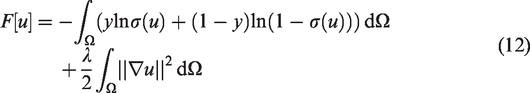
The most popular framework is the minimization of an energy functional like

\min_{u} \sum_{i = 1}^{N} L (u (x_{i}), y_{i}) + λ S (u)

(2)

where L(u, y) is the loss function and S(u) is a regularizer. For the continuous case, however, we have:

\min_{u} \int_{Ω} L (u, y) d Ω + λ S (u)

(3)

The basic idea behind this variational model is to penalize wrong predictions through the loss function while allowing some relaxation through the regularizer. This is, the regularizer allows to control the smoothness of u representing the separating hypersurface. The regularizer also helps by making the problem well-posed and preventing overfitting. We will use a Lebesgue integrable function R(u) > 0 to somehow measure the complexity of u. The variational model (3) is then transformed into

\min_{u} F [u] \equiv \int_{Ω} L (u, y) d Ω + λ \int_{Ω} R (u) d Ω

(4)

A probabilistic interpretation of (4) is to notice that the empirical risk of choosing u among a space of hypothesis functions $H$ is defined as the expectation of the loss function $E [L (u, y)] = \int_{Ω} L (u, y) d Ω$ . Therefore, minimizing the regularized empirical risk, amounts to solving the following minimization problem:

u^{*} = \arg \min_{u \in H} F [u]

(5)

Radial basis function approximation

Finding $u^{*}$ in (5) involves solving numerically a partial differential equation (PDE). Due to the nature of the problem, it is be not possible to use traditional methods such as the finite difference method. Therefore, we turn to using a collocation method to reduce the problem to a set of algebraic equations. To this end, we choose a set of radial basis functions (RBF) to approximate u(x) as a weighted sum of functions $ϕ_{i} (x)$ and weights w_i for $i = 1, \dots, N$ . There are many possible choices for $ϕ_{i} (x)$ . However, the Gaussian RBF kernel is probably the most known and widely used and therefore the one we chose to use all along this work. Thus, we write

u (x) = \sum_{i = 1}^{N} w_{i} ϕ_{i} (x_{i})

(6)

and

ϕ_{i} (x) = e^{- c | | x - x_{i} | |^{2}}

(7)

where c > 0 is a constant that we are free to choose and

| | \cdot | |

the Euclidean norm. We will call c the fitting degree of our model.

Notice that in (7), the centers of the RBFs are the data observations x_i. Due to this, the model will make predictions based on the Euclidean distance between points which class is known, and the new input for which its class is unknown while assigning a weight to each point. Therefore, some points will be more important than others when making the predictions. A similar idea to the one used in SVM.

Cross entropy as fitting term

A correct selection of the loss function in (4) is vital for the performance of the model. Here, since the model will be used for binary classification, we take a Bernoulli variable $Y \in {0, 1}$ . Generalization to multiclass is straightforward.

The criteria to select an appropriate loss function is that it must maximize the likelihood that, given parameters w_i, the model results in a prediction of the correct class for each input sample and this likelihood should be a function of these parameters. This can be achieved by the minimization of the cross-entropy⁶ (also called negative log-likelihood) that effectively maximizes the likelihood. This function is given by:

L (u, y) = - y \ln σ (u) - (1 - y) \ln (1 - σ (u))

(8)

where

σ (u) = e^{u} / (1 + e^{u})

is the sigmoid function.

L₂ function regularization

With the loss function for binary classification already chosen, we now proceed to select a regularizer. Most machine learning models mainly use parameter regularization by regularizing the weight vector $w = (w_{1}, \dots, w_{N})$ instead of u. This is the case of the regularizer

S (w) = \int_{Ω} | | w | |^{2} d Ω

(9)

also known as ridge regression⁷ or Tikhonov regularization. This type of regularization helps the algorithm to distinguish between those inputs with high variance from the ones with small variance.

There is also the case of

S (w) = \int_{Ω} | | w | | d Ω

(10)

known as LASSO (Least Absolute Shrinkage and Selection Operator) regression.^8,9 The key difference here is that LASSO shrinks the less important feature’s coefficient to zero thus, removing some features altogether.

More recently, Belkin et al.¹⁰ proposed that under the assumption that the support of the marginal distribution of the dataset is a compact manifold embedded in $ℝ^{N}$ then a suitable regularizer is given by

S (u) = \frac{1}{2} \int_{Ω} | | \nabla u | |^{2} d Ω

(11)

Lin et al.¹¹ took this idea further and explored with success the use of the Total Variation and Euler elastica as regularizers.

We argue that this way of directly regularizing the separating hypersurface u is better than regularizing the vector of parameters w. Our argument is that while penalizing w has the objective of controlling the values w_i individually which in some cases may growth indiscriminately, penalizing u or its gradient as in (11) has the intention of controlling the smoothness of the separating hypersurface. The second, has the immediate impact of reducing overfitting.

The model

Let $u : Ω \subset ℝ^{d} \to ℝ$ be the classification function and let $y \in {0, 1}$ be the target values. Let $σ (u)$ to represent the probability that an input u(x) is classified as true or positive i.e. y = 1. Let

\begin{array}{l} F [u] = - \int_{Ω} (y \ln σ (u) + (1 - y) \ln (1 - σ (u))) d Ω \\ + \frac{λ}{2} \int_{Ω} | | \nabla u | |^{2} d Ω \end{array}

(12)

Then our supervised learning models amounts to solving (5) with $F [u]$ defined above.

Analysis of the model

Existence and uniqueness of a minimizer

In this section, we shall determine existence of a minimizer of our model. Our proof of existence consists in showing that some minimizing sequence ${u_{k}}_{k \geq 0}$ actually does converge to a minimizer. We will show that the minimizing sequence is bounded and therefore there exists a subsequence which is convergent, given the right hypothesis. Theorem 3.1

(Existence of a Minimizer). Let $Ω \subset ℝ^{N}$ be a bounded open set with a C¹ boundary and $λ > 0$ constant. Furthermore, assume that $L : Ω \times ℝ \times ℝ$ is a non-negative convex function that is Lipschitz continuous. Then the functional

F [u] = \int_{Ω} (L (u, y) + \frac{λ}{2} | | \nabla u | |^{2}) d Ω

has at least one minimizer $u \in X$ , where

X = {u \in W^{1, 2} (Ω) | u = v on \partial Ω in the sense of a trace}

for

v \in W^{1, 2}

. Proof.

Assume $m = \inf_{u} F [u]$ is finite. If it were not, we could just pick any u and we would be done. Let ${u_{k}}_{k \geq 0}$ be a minimizing sequence such that $u_{k} \in X$ . By the definition of X, we know that for any fixed $\hat{u} \in X$ then $u_{k} - \hat{u} \in W_{0}^{1, 2}$ . Applying the Poincaré inequality yields

\begin{array}{l} | | u_{k} | |_{W^{1, 2} (Ω)} - | | \hat{u} | |_{W^{1, 2} (Ω)} \leq | | u_{k} - \hat{u} | |_{W^{1, 2} (Ω)} \\ \leq c | | \nabla u_{k} - \nabla \hat{u} | |_{L^{2} (Ω)} \\ \leq c | | \nabla u_{k} | |_{L^{2} (Ω)} + c | | \nabla \hat{u} | |_{L^{2} (Ω)} \end{array}

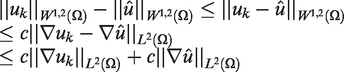
where c is some positive constant. We know that

F [u] = \int L (u, y) d Ω + c | | \nabla u | |_{L^{2} (Ω)}^{2} \geq c | | \nabla u | |_{L^{2} (Ω)}

and so, we can derive

| | u_{k} | |_{W^{1, 2} (Ω)} \leq c | | \nabla u_{k} | |_{L^{2} (Ω)} + β \leq F [u_{k}]

for constant

β = | | \hat{u} | |_{W^{1, 2} (Ω)} + c | | \nabla \hat{u} | |_{L^{2} (Ω)}

Since u_k is a minimizing sequence for m finite, we have that $| | u_{k} | |_{W^{1, 2} (Ω)}$ is bounded. Consequently there must exist a subsequence ${u_{k_{i}}}_{k_{i} \geq 0}$ such that $u_{k_{i}} ⇀ \bar{u} in W^{1, 2} (Ω)$ , for some $\bar{u}$ , in the sense that $u_{k_{i}} ⇀ \bar{u}$ and $\nabla u_{k_{i}} ⇀ \nabla \bar{u}$ in $L^{2} (Ω)$ .

To show that $F [u_{k_{i}}] \to F [\bar{u}]$ , it is enough to show that $F [u]$ is lower semicontinuous to deduce $F [\bar{u}] \leq m$ . To this end, we must prove two things individually:

\underset{k \to \infty}{\lim \inf} \int_{Ω} | \nabla u_{k_{i}} | d Ω \geq \int_{Ω} | \nabla \bar{u} | d Ω

(13)

and

\lim_{k \to \infty} \int_{Ω} L (u_{k}, y) d Ω \geq \int_{Ω} L (\bar{u}, y) d Ω

(14)

This is straightforward using the convexity of the functionals. In other words, we know that for some $φ \in W^{1, 2}$ and $ν \in L^{2}$ , the following is true:

| \nabla u_{k_{i}} | \geq | \nabla \bar{u} | + 2 {〈 ν, \nabla u_{k_{i}} - \nabla \bar{u} 〉}_{L^{2}}

(15)

and

L (u_{k}) \geq L (\bar{u}) + {〈 φ, u_{k} - \bar{u} 〉}_{W^{1, 2}}

(16)

By taking the limit $k \to \infty$ on both sides of (15) and (16) and since $u_{k} ⇀ \bar{u}$ in $W^{1, 2}$ and $\nabla u_{k_{i}} ⇀ \nabla \bar{u}$ in $L^{2} (Ω)$ , it follows immediately that

\lim_{k \to \infty} \int_{Ω} {〈 ν, \nabla u_{k_{i}} - \nabla u 〉}_{L^{2}} d Ω = 0

(17)

\lim_{k \to \infty} \int_{Ω} {〈 φ, u_{k} - \bar{u} 〉}_{W^{1, 2}} d Ω = 0

(18)

and therefore (13) and (14) are satisfied. To end the proof, note that since

{u_{k_{i}}}_{k_{i} \geq 0}

was a minimizing sequence,

F [u_{k_{i}}] \to m

and

F [u]

is lower semicontinuous, then we must have

F [\bar{u}] = m

. □

This completes our proof for the existence of a minimizer. We will end this section by stating a theorem about the uniqueness of the minimizer which follows by the convexity of the functional. The proof is elementary and therefore will not be presented. Theorem 3.2

(Uniqueness of Minimizer). If L is strictly convex, then the functional $F [u]$ in Theorem 3.1 has a unique solution.

The solution

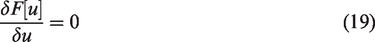
In order to solve the expression in (4), we proceed to compute the functional derivative and equate to zero i.e. the first order optimality condition

\frac{δ F [u]}{δ u} = 0

(19)

To this end, let $R = R (u, \nabla u)$ and $L (u) = L (u, y)$ with y fixed. Then, the functional derivative in (19) yields the Euler Lagrange equation:

\frac{δ F}{δ u} = \frac{\partial f}{\partial u} - \nabla \cdot \frac{\partial f}{\partial \nabla u} = [\frac{\partial L}{\partial u} + λ \frac{\partial R}{\partial u}] - \nabla \cdot [\frac{\partial L}{\partial \nabla u} + λ \frac{\partial R}{\partial \nabla u}]

(20)

= \frac{d L}{d u} + λ \frac{d R}{d u} - λ \nabla \cdot \frac{\partial R}{\partial \nabla u} \frac{d L}{d u} + λ (\frac{d R}{d u} - \nabla \cdot \frac{\partial R}{\partial \nabla u})

where

f = f (x, u (x), \nabla u (x))

. After equating to zero the last equation, our original problem is then reduced to solving the following PDE for particular choices of L and R:

\frac{d L}{d u} + λ (\frac{d R}{d u} - \nabla \cdot \frac{\partial R}{\partial \nabla u}) = 0

(21)

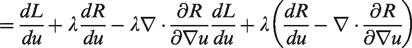
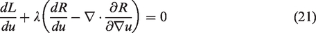
From the definition of L in (8) we get

\frac{d L}{d u} = σ (u) - y

(22)

and for

R (u, \nabla u) = | | \nabla u | |^{2}

as defined in (11) we get

\frac{d R}{d u} - \nabla \cdot \frac{\partial R}{\partial \nabla u} = \frac{d}{d u} \frac{| | \nabla u | |^{2}}{2} - \nabla \cdot \frac{\partial}{\partial \nabla u} \frac{| | \nabla u | |^{2}}{2} = - Δ u

(23)

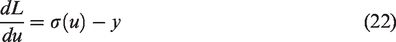
Then the condition of optimality is the elliptic PDE

σ (u) - y - Δ u = 0

(24)

To solve the problem numerically, we recall that u depends on w. Then the problem is reduced to finding the weight vector $w^{*}$ which appropriately satisfies (25).

\underset{Function to fit}{\underset{︸}{σ (u) - Δ u}} = \underset{Targets}{\underset{︸}{y}}

(25)

Having N datum pairs (x_i, y_i) it is possible to write the problem of finding $w^{*}$ as a least squares problem (LSQP). Let $g (x_{i}, w) = σ (u (x_{i}, w)) - Δ u (x_{i}, w)$ , then the LSQP is:

w^{*} = \arg \min_{w} \sum_{i = 1}^{N} [y_{i} + Δ u (x_{i}, w) - σ (u (x_{i}, w))]^{2}

(26)

= \arg \min_{w} \sum_{i = 1}^{N} [y_{i} - g (x_{i}, w)]^{2}

(27)

= \arg \min_{w} \sum_{i = 1}^{N} [y_{i} - g_{i} (w)]^{2}

(28)

= \arg \min_{w} S (w),

(29)

Note we have defined $g_{i} (w) = g (x_{i}, w)$ to obtain the third step. In our particular case, we solve this problem via the Levenberg-Marquardt (LM) method.¹² Notice that a damping parameter η that have to be selected is introduced by the LM method.

Training with LM

The LM algorithm consists in estimating $w^{*}$ by following a sequence of estimations, each better than the previous one, so that $w^{(j + 1)} = w^{(j)} + δ$ and therefore $w^{(n)} \to w^{*}$ as $n \to \infty$ . We can determine $δ$ by looking at the linearisation of $g_{i} (w + δ) = g (x_{i}, w + δ)$ which is given by

g_{i} (w + δ) \approx g_{i} (w) + \nabla g_{i} (w) δ

(30)

\nabla g_{i} (w) = \nabla_{w} g (x_{i}, w)

(31)

Equation (31) is the gradient of g with respect to w. By looking at the expression of the linearisation of the function, we can expand it to get

S (w + δ) \approx \sum_{i = 1}^{N} (y_{i} - g_{i} (w) - \nabla g_{i} (w) δ) = | y - g (w) - J δ |^{2} = \dots = {[y - g (w)]}^{T} [y - g (w)] - 2 {[y - g (w)]}^{T} J δ + δ^{T} J^{T} J δ .

(32)

Taking the derivative of (32) with respect to δ, we see that

(J^{T} J) δ = J^{T} [y - g (w)]

(33)

must be satisfied. This last line can also be interpreted as “solve for

δ

”. It is desirable, however, this method to converge smoothly to a solution and so LM added a damping factor to the equation above. Therefore the LM algorithm at each step will solve a damped version of the previous equation:

[J^{T} J + η diag (J^{T} J)] δ = J^{T} [y - g (w)]

(34)

where η is a damping parameter which may be fixed or calculated at each iteration. Finally, we can give the algorithm to train our model along with the mathematical expressions used.

Algorithm 1: Training the model (Levenberg-Marquardt)

Data:

x such that $x = {(x_{1}, \dots, x_{N})}^{T}$ is the matrix of observations

λ is a regularization parameter

c is the fitting degree

η is a dampening parameter

M is the number of iterations

Result: The weight vector $w^{*}$

begin

$j \leftarrow 0$ ;

$w^{(0)} \leftarrow {(0, \dots, 0)}^{T}$ ;

while j < M do

Solve $[J^{T} J + η diag (J^{T} J)] δ = J^{T} [y - g (w)]$ for $δ$ $w^{(j + 1)} \leftarrow w^{(j)} + δ$

We now proceed to give the expressions used in the algorithm.

\begin{array}{l} y = [y_{1}, \dots, y_{N}] \\ g (w) = {[g_{1} (w), \dots, g_{N} (w)]}^{T} \\ J = {[\nabla g_{1} (w), \dots, \nabla g_{N} (w)]}^{T} \\ \nabla g (w) = \nabla_{w} σ (u) - λ \nabla_{w} Δ u \\ \nabla_{w} σ (u) = σ (u) (1 - σ (u)) {[ϕ_{1}, \dots, ϕ_{N}]}^{T} \\ \nabla_{w} Δ_{u} = [Δ ϕ_{1}, \dots, Δ ϕ_{N}] \\ Δ ϕ_{i} = c (c | x - x_{i} |^{2} - d) ϕ_{i} \end{array}

Results

In this section we present some results to illustrate the performance of our Regularized Logistic Regression (RLR) model. We tested RLR against the nine binary datasets shown in Table 1. For comparison purposes we decided to compare the results against those obtained from L₁ and L₂ regularized logistic regression (classical regularization over the weights), SVM and NN.

Table 1.

In this Table, we present the datasets we used for testing.

Data	Dimension	Number of samples
Australian	14	690
BT	4	748
BC	30	569
Bupa	6	345
German	24	1000
Haberman	3	306
Heart	13	270
Sonar	60	208
VC	6	310

BT: blood transfusion; BC: breast cancer; VC: vertebral column.

The datasets were standardized, i.e. all features in each dataset were centered to zero mean and unit variance. No dimensionality reduction was used in the experiments.

For each dataset we calculated two metrics: Accuracy and Area under the ROC curve (AUC).¹³ The 5-fold cross validation scheme was also used in both metrics. In the experiments, we took care of selecting the different parameters of each method fairly. For our RLR model we have to choose the triplet $(c, λ, η)$ ; where c is the fitting degree, λ is the regularization parameter and η is the LM dampening parameter. For classical L₁ and L₂ regularized logistic regression, we have to select the regularization parameter C. For a RBF-kernel SVM, we have to select the pair $(C, γ)$ ; where C is the penalty parameter while γ is the kernel coefficient. The architecture of the NN is a multi-layer perceptron with one hidden layer of 100 nodes which depends on a regularization term α. Both regularized logistic models, as well as SVM and NN are implementations of the Python library sklearn.¹⁴ The parameters for each model were chosen by the following methodology:

RLR

The triplet $(c, λ, η)$ is searched as follows:

c is searched on (0, 5) with step $= \ln 2$ .

λ is searched on $[0, 10]$ with step $= 1$ .

η = 1 was used for each dataset. This value was empirically found to be the best.

L₁ and L₂ regularized logistic regression

C is searched on (0, 5) with step $= \ln 2$ .

SVM

The pair $(C, γ)$ is searched as follows:

C is searched on (0, 5) with step $= \ln 2$ .

$γ = 1 / m$ was used for all datasets, where m is the number of features of the dataset. This value was empirically found to be the best.

NN

The parameter $α = 0.001$ was used for all datasets.

Accuracy

In Table 2 we present the classification results in terms of accuracy. The first thing to notice is that both classical L₁ and L₂ regularized logistic regression models performed poorly. Other than the Heart dataset, where the accuracy was similar to that one obtained from the other models (meaning that the Heart dataset is linearly separable), they consistently delivered low accuracy values. Due to this, we will not discuss more about these two models in the rest of the paper.

Table 2.

The accuracy (%) of each method is outlined in this table.

Dataset	L ₂	L ₁	RLR	SVM	NN
Australian	81.19	85.49	86.66	86.81	87.82
BT	77.55	77.92	78.22	78.22	77.28
BC	94.19	95.77	97.71	98.74	98.26
Bupa	61.13	64.43	72.46	72.46	71.01
German	75.12	75.28	76.00	76.60	78.30
Haberman	71.80	71.62	73.54	73.87	74.52
Heart	84.00	84.06	84.22	84.87	84.01
Sonar	43.36	44.45	88.43	88.92	87.46
VC	78.55	78.94	86.77	85.48	83.87

On the other hand, although RLR just outperformed SVM and NN on three datasets out of nine, in general we see that RLR is quite competitive when compared against these two fully stablished methods.

We also calculated the accuracy distances for a better insight. This is, the absolute value of the residual between each method’s accuracy and the one of the top performer. The results are shown in Table 3. On average RLR was down by 0.73%, SVM by 0.51% and NN by 0.89%. With this in mind, we can say that in terms of accuracy, SVM is the best method, while RR is second and NN comes a close third.

Table 3.

The absolute value of the residual between the method’s accuracy and the method with the highest accuracy.

Dataset	RLR	SVM	NN
Australian	1.16	1.01	0.0
BT	0.0	0.0	0.94
BC	1.03	0	0.48
Bupa	0.0	0.0	1.45
German	2.3	1.7	0.0
Haberman	0.98	0.65	0.0
Heart	0.65	0.0	0.86
Sonar	0.49	0.0	1.46
VC	0.0	1.29	2.90
Average distance	0.73	0.51	0.89

AUC score

The AUC score is another way to evaluate the performance of a classifier.¹⁵ In Table 4, we present the AUC values obtained for the different models and datasets. We also applied a similar analysis to the one presented above for the accuracy values. This is, we calculated the AUC distances (the differences between AUC values) for each dataset. In order to compare the models, we computed the sum of the distances (instead of the averages) obtaining the values that can be seen at the bottom of Table 5: RLR = 0.12, SVM = 0.02 and NN = 0.17. The result suggest that SVM is the best performer, RLR the second and NN is third. This is consistent with what was obtained when analyzing the accuracy values.

Table 4.

In this Table, we show the values for the area under the ROC curve (AUC) for each method over each dataset. Between brackets is the assigned grade; A being excellent performance, while F is catalogued as a fail. Bold numerals are the highest values.

Dataset	RLR	SVM	NN
Australian	0.86 (B)	0.87(B)	0.87 (B)
BT	0.58 (F)	0.61 (D)	0.55 (F)
BC	0.97 (A)	0.98 (A)	0.98 (A)
Bupa	0.70 (C)	0.70 (C)	0.68 (D)
German	0.68 (D)	0.69 (D)	0.70 (C)
Haberman	0.56 (F)	0.55 (F)	0.54 (F)
Heart	0.82 (B)	0.84 (B)	0.83 (B)
Sonar	0.88 (B)	0.89 (B)	0.88 (B)
VC	0.82 (B)	0.84 (B)	0.79 (C)

Table 5.

This Table shows the AUC distances. This is, the absolute value of the residual between each method’s AUC and the method with the highest AUC for each dataset.

Dataset	RLR	SVM	NN
Australian	0.01	0.0	0.0
BT	0.03	0.0	0.06
BC	0.01	0.0	0.0
Bupa	0.0	0.0	0.02
German	0.02	0.01	0.0
Haberman	0.0	0.01	0.02
Heart	0.02	0.0	0.01
Sonar	0.01	0.0	0.01
VC	0.02	0.0	0.05
Sum of distances	0.12	0.02	0.17

Grading

Here we introduce a more intuitive analysis based on the AUC. We consider this analysis more robust than the previous. The analysis consists in assigning a “grade” to the results of a classifier by specifying the following grading scheme:

Grade = {\begin{array}{l} Excellent (A) 0.9 \leq AUC \leq 1 \\ Good (B) 0.8 \leq AUC < 0.9 \\ Fair (C) 0.7 \leq AUC < 0.8 \\ Poor (D) 0.6 \leq AUC < 0.7 \\ Fail (F) 0.5 \leq AUC < 0.6 \end{array}

By following the above grading scheme, we are partitioning discretely the interval $[0, 1]$ and assigning each sub-interval a grade. Therefore, small variations within the sub-intervals will be neglected making the evaluation more robust. In Table 4 we see that each of the AUC scores has a letter assigned to it which represents the grade the method received on that particular dataset. To summarize, we arranged the number of times a method received a particular grade in Table 6 and to obtain a quantitative measure, we assigned each grade a value: A = 1, B = 2, $\dots$ , F = 5.

Table 6.

The number in each column indicates the number of times each method got the grade on the leftmost column. By assigning the values A = 1, B = 2, C = 3, D = 4, F = 5, we can calculate a weighted final grade.

Grade	RLR	SVM	NN
A	1	1	1
B	4	4	3
C	1	1	2
D	1	2	1
F	2	1	2
Weighted grade (lower is better):	26	25	29

In the bottom row in Table 6 it is the weighted total of the grades. The lowest the total value, the better the method. Again SVM obtained the best score. This time, RLR came a close second with only a 1 point difference and NN was very far by 4 points.

Conclusion

In this work, we have shown the way a new method for the supervised learning problem can be developed from a variational point of view. We have seen that it is very possible to formally formulate the problem as the minimization of a functional which has an associated PDE that describes the necessary conditions that a minimizer must meet. This equation proved to be easy to solve numerically with the least-squares algorithm Levenberg Marquardt. Tests were conducted and we compared the performance of our own model with the classical L₁ and L₂ regularized logistic regression models, NN and an RBF SVM. Both classical regularized models performed poorly as expected in every non linearly separable dataset. By regularizing u instead of w we were able to improve results substantially. From this analysis, it was clear that while SVM beat both our model and NN, our model outperformed NN while staying relatively close to the performance of SVM.

Finally, like all formal analyses, it was necessary to prove the existence and uniqueness of a solution for our functional. The validity of this claim turned out to be true by Theorem 3.1. Even more, we were able to prove that, indeed, a solution of the PDE is a minimizer of a functional, thereby, formally justifying our argument that we could minimize our functional by solving the condition of optimality. By and large, our true intention was to showcase that a variational approach can be used and should be used for tackling the supervised learning problem. A variational approach encompasses the areas of functional analysis and the calculus of variations, both of which permitted us to make this work possible. Using the methods of the calculus of variations we were able to guarantee a solution which was facilitated by the theory of functional analysis. Therefore, we can only conclude that the choice of a variational approach in solving the supervised learning problem was satisfactory.

The implementations for the RLR model, benchmarking scripts and datasets may all be found at https://github.com/carlosb/thesis.

Footnotes

Declaration of Conflicting Interests

The author(s) declared no potential conflicts of interest with respect to the research, authorship, and/or publication of this article.

Funding

The author(s) received no financial support for the research, authorship, and/or publication of this article.

ORCID iDs

Carlos Brito-Pacheco

Carlos Brito-Loeza

Appendix 1.

In this section, we aim to derive the weak Euler-Lagrange equation and see that solutions of it are in fact minimizers of $F [u]$ . We shall require that the supervised learning Lagrangian be in in the class of functions C¹ and its derivatives satisfy growth conditions.

References

Singh

Thakur

Sharma

A review of supervised machine learning algorithms. In: 3rd International conference on computing for sustainable global development (INDIACom), New Delhi, 16–18 March 2016, pp.1310–1315. IEEE.

Fernández-Delgado

, et al. Do we need hundreds of classifiers to solve real world classification problems. J Mach Learn Res 2014; 15: 3133–3181.

Kotsiantis SB. Supervised machine learning: a review of classification techniques, Informatica, 2007; 31: 249–268.

Caruana

, and Niculescu-Mizil A. An empirical comparison of supervised learning algorithms. In: Proceedings of the 23rd international conference on machine learning, 2006. New York: ACM.

Schwenker

Trentin

Pattern classification and clustering: a review of partially supervised learning approaches. Pattern Recogn Letters 2014; 37: 4–14.

Shore

Johnson

Axiomatic derivation of the principle of maximum entropy and the principle of minimum cross-entropy. IEEE Trans Inform Theory 1980; 26: 26–37.

Ehsanes AK, Saleh Md, Arashi Mohammad, Kibria BM. Golam. Theory of Ridge Regression Estimation with Applications. John Wiley and Sons, 2019.

Santosa

Symes

WW.

Linear inversion of band-limited reflection seismograms. SIAM J Sci Stat Comput 1986; 7: 1307–1330.

Tibshirani

Regression shrinkage and selection via the lasso. J R Stat Soc, Series B 1996; 58: 267–288.

10.

Belkin

Niyogi

Sindhwani

Manifold regularization: a geometric framework for learning from labeled and unlabeled examples. J Mach Learn Res 2006; 7: 2399–2434.

11.

Lin

Xue

Wang

, et al. Supervised learning via Euler’s elastica models. J Mach Learn Res 2015; 16: 3637–3686.

12.

Moré JJ (1978) The Levenberg-Marquardt algorithm: Implementation and theory. In: Watson GA (eds) Numerical Analysis. Lecture Notes in Mathematics, vol. 630. Berlin, Heidelberg: Springer.

13.

Hanley

McNeil

BJ.

The meaning and use of the area under a receiver operating characteristic (ROC) curve. Radiology 1982; 143: 29–36.

14.

Pedregosa

, et al. Scikit-learn: machine learning in python. J Mach Learn Res 2011; 12: 2825–2830.

15.

Fawcett

An introduction to ROC analysis. Pattern Recogn Lett 2006; 27: 861–874.