Sage Journals: Discover world-class research

Abstract

In the k-coverage process of target nodes, substantial data redundancy occurs, which leads to the phenomenon of congestion, reducing the network communication capability and coverage as well as accelerating network energy consumption. Therefore, this article proposes an Optimization Coverage Conserving Protocol with Authentication. This protocol provides a solution to obtain the largest coverage probability for multi-nodes. In the optimization and authenticated calculation, the protocol provides the calculation method and verification process of the expected value of multi-node coverage; when the moving target nodes are continuously covered, this protocol provides a process to solve for the focused target nodes; when there is redundancy coverage, this article provides a process to calculate the coverage probability when any sensor node is covered by a redundant node. Furthermore, through comparisons of the coverage quality and network lifetime with other algorithms, the performance indexes of this protocol have been substantially increased by the simulation experiment, which verified the effectiveness and viability of the protocol in this article.

Keywords

Wireless sensor networks conserving protocol optimization coverage coverage quality network lifetime

Introduction

A wireless sensor network is a new type of network architecture that is connected by a self-organizing multi-hop, which is formed by thousands of sensor nodes. The physical world and information world are organically integrated and involve data acquisition, data calculation, data communication, and data storage.^1,2 As a result of the rapid development of information technology, a wireless sensor network can be applied in all types of engineering fields, such as military affairs, environmental monitoring, disaster relief, smart homes, health care, agricultural production, and transportation.^3,4

Energy consumption and coverage quality are the two key issues in wireless sensor network research,^5,6 the behavioral characteristic of which is the deployment of sensor nodes. The problem of energy consumption includes how to effectively suppress rapid energy consumption of sensor nodes to extend the network lifetime and improve Internet service. The coverage quality and network energy consumption are dependent on the deployment probability of sensor nodes.^4,7 In general, as a result of the limitations of the topographic and geomorphic conditions and environmental factors, we typically use the methods of stochastic deployment to handle the deployment of sensor nodes. Moreover, because of randomness, it is not possible to predict the specific location of sensor nodes during deployment, which indicates that there are several or enough sensor nodes in a specific monitoring area or at a monitoring point. It may ultimately form k-degree coverage.^8–10 Another case is that during random deployment, it is possible that some of the monitoring areas and monitoring points may not be covered by the sensor nodes, which may form a coverage hole and can only be covered by adding sensor nodes to produce effective coverage. Both of these cases may complete coverage; however, several shortages remain. First, many sensor nodes cluster at a very high density; thus, there will be substantial redundant information, which will cause congestion in the communication linkage, suppress the expandability of the network, lower the service quality of the network, and shorten the lifetime of the network. Second, when the focus target nodes are in the coverage hole, real-time monitoring and coverage cannot be completed. Moreover, with respect to the sensor nodes, they cannot provide correct data to the sink nodes, and there will be deviations and uncertainties in the data that the sink nodes have collected. Third, after several rounds, the sensor nodes will exhibit heterogeneity. Because of this heterogeneity, the coverage ranges of the nodes will be changed. As long as the state of the target nodes changes from the coverage state to the noncoverage state, the data that the target nodes collected will lose their meaning. Fourth, the intrinsic of the coverage is not to produce complete coverage of all target nodes; rather, it aims to produce effective coverage of the focus target nodes. Moreover, the intrinsic of the effective coverage is that when the focus target nodes pass through the monitoring area, the sensor nodes will first complete coverage and simultaneously wake up their joint nodes to complete linkage coverage. The data collected from the moving goal nodes will subsequently be uploaded to the sink nodes.

Regarding the deficiencies and shortcomings of the previously described research, the main contributions of this article will be presented as follows:

Following an assessment and analysis of the relevant domestic and international literature, we propose the Optimization Coverage Conserving Protocol with Authenticated (OCPA) algorithm in this article, which was facilitated by theoretical ideas from the literature.

In the monitoring area, this article selects k nodes at random as the object of research. Based on the probability theory and according to the perceived radius of the sensor nodes, this article provides a solving method and process of the expected value when there are k nodes covered jointly.

When the target nodes are covered by joint nodes or single nodes, this article provides comparative methods of the awareness intensity. Moreover, by limiting the value range of the adjustable parameter λ, this article provides a judgment method of the redundancy coverage of any sensor node covered by redundant nodes.

Through a simulation experiment and by comparison to other algorithms, we verify the effectiveness and feasibility of the OCPA algorithm.

Relative literature

The technique of coverage control represents essential research regarding the wireless sensor network and is also currently one of the hotspot problems in the wireless sensor network. The coverage quality will affect the lifetime of the network. In recent years, many experts and scholars at home and abroad have thoroughly and carefully conducted many studies. Zhao et al.¹¹ propose an optimization strategy for the coverage algorithm based on Voronoi. Satisfying the condition of a specific coverage quality, the algorithm may add work nodes to the coverage hole to improve the current coverage probability; furthermore, it will search for reasonable information regarding the repairing site to guarantee the connection of the whole network. Meng et al.¹² provide a constructive method of the connected coverage protocol. The protocol provides the proportional relation between the network coverage quality as well as the network and performance indexes of all of the parameters of the network system; moreover, it creates the scheduling control algorithm (SCA), which uses the fewest nodes needed to guarantee the connection of the whole network system. Mini et al.¹³ introduces artificial intelligence algorithms, that is, the swarm intelligence algorithm and granule algorithm, to complete node deployment of the whole network monitoring area; in the stage of coverage optimization, the whole coverage is optimized by the two artificial intelligence algorithms and ultimately attains complete coverage of the monitoring area; with respect to energy consumption, it completes scheduling conversion of the node energy via heuristic node scheduling, which extends the lifetime of the network. Hanid et al.¹⁴ also include the Voronoi as the research objective; it solves the information of the wire rod site formed by the geometric variation in the Voronoi and sensor nodes and ultimately completes coverage of the monitoring area. Tseng et al.² include a partial coverage optimization and constitute the partial α coverage; after a series of calculations and optimizations of the α, complete coverage optimization is ultimately achieved. These algorithms all achieved effective coverage of the monitoring area to some extent; however, they have mutual problems in that all of the algorithms require a large number of calculations and are more complex, as well as the scalability of the wireless sensor network is worse. Li et al.¹⁵ and Zhibo et al.¹⁶ effectively compute the goal nodes by utilizing the different angles of the sector determined by the sensor nodes and goal nodes and provide a method for computing the coverage probability of different monitoring areas. These algorithms have better feasibility and higher reliability; however, the network models and algorithms are too complex when they are implemented in research. Tseng et al.,² Hanid et al.,¹⁴ and Li et al.¹⁵ include static goal nodes as the research objective, and Zhibo et al.¹⁶ do not consider what the k-barrier coverage will be when the moving target nodes are the concerned goal nodes. Li et al.¹⁷ propose a polytypic target coverage algorithm based on linear programming. The algorithm utilizes the clustering structure to solve the polytypic target coverage problem. By computing the coverage ability and residual energy of the sensor, it completes polytypic target optimization coverage via linear programming. Otero et al.¹⁸ propose the event probability-driven mechanism (EPDM) algorithm, and this algorithm calculates the coverage probability and expected value of the sensor nodes with the probability model; it subsequently optimizes the result and achieves optimal coverage. These two algorithms achieve optimal coverage and extension of the network lifetime; however, the coverage condition is relatively hasher, and the calculations of the algorithms are substantially more complex.

To improve the effective coverage of the monitoring area, and on the basis of Li et al.¹⁵ and Zhibo et al.,¹⁶ this article proposes an OCPA. The protocol described in this article calculates the coverage expected value of the moving target nodes to the sensor nodes with the relative knowledge of the probability. Moreover, it provides a solving process of the coverage expected value of the target nodes to the sensor nodes for the first time. In terms of energy, on the basis of the analysis of all sensor node energies in the whole network, the algorithm performs an energy comparison under the multilateral and unilateral connections, that is, the energy consumption of the data in the multicast nodes is less than that in the unilateral nodes. In terms of energy conversion, the algorithm completes energy conversion among nodes using the self-scheduling mechanism, which extends the lifetime of the network. Finally, through simulation experiments and comparison with other algorithms, the effectiveness and stability of the OCPA algorithm are verified.

Prerequisite knowledge

To simplify the description, the following symbol will be used ||M|| to represent the area of ||M||. E[X] represents the expected value of the random variable, X. P{A} is the probability that the event A may occur. Z is the conjugate complex number of Z. $fourier (f (x)) = \int_{- \infty}^{+ \infty} f (x) \exp (- iwx) d x = F (w)$ ; this function is the continuous Fourier transform of the function f(x). $ifourier (F (w)) = (1 / 2 π) \int_{- \infty}^{+ \infty} F (w) \exp (ixw) d w = f (x)$ is the continuous inverse discrete Fourier transform.

Definition 1

As for any one point q in the area M, if the joint sensing intensity of q meets I(q) ≥ I_th, then point q may be covered (i.e. the event that occurs at point q may be monitored); otherwise, point q is not covered. I_th is the threshold of the sensing intensity (which is settled according to the character and application demands of the users). Thus, the coverage situation of q may be represented as

Cov (q) = {\begin{matrix} 1 I (q) \geq I_{th} \\ 0 I (q) \leq I_{th} \end{matrix}

(1)

In the binary sensing model, the sensing area of node s is a circle, of which point s is the center of the circle and r_s is the radius of the circle (the circle is defined as C(s, r_s) and r_s ≤ R_s). The points in the area of C(s, r_s) may all be covered by node s; however, any point beyond C(s, r_s) cannot be covered by node s. Thus, r_s in the binary sensing model meets the relation e^−αrs = I_th, that is, r_s = −ln(I_th)/α.

Definition 2

The proportion of the monitoring area M that is covered by the network occupies all of the monitoring area M is referred to as the coverage quality. That is

η = \int \int_{M} \frac{Cov (q)}{‖ M ‖} d M

(2)

A sensor network may be abstracted as an undirected graph G = (V, E), in which V is the set of nodes and E is the set of the undirected edge.

Definition 3

The specific value of the effective coverage of the sensor nodes with the coverage area of the sensor nodes

P_{e} = \frac{area ((⋃_{i = 1, 2, \dots, N} s_{i}) ⋂ area (S))}{area (⋃_{i = 1, 2, \dots, N} s_{i})}

(3)

Definition 4

In the target set, any one of the target nodes is covered by at least one sensor node p; when the target node is covered by several joint sensor nodes, the coverage probability will be

p_{n} = 1 - {(1 - p)}^{N}

(4)

p_n is the joint coverage proportion, p is the coverage rate of any one of the sensor nodes, and N is the number of sensor nodes.

Theorem 1

The sensor nodes randomly deployed in the monitoring area comply with the probability density, λ. Moreover, N(s) is the Poisson distribution of the random variables.

Proof

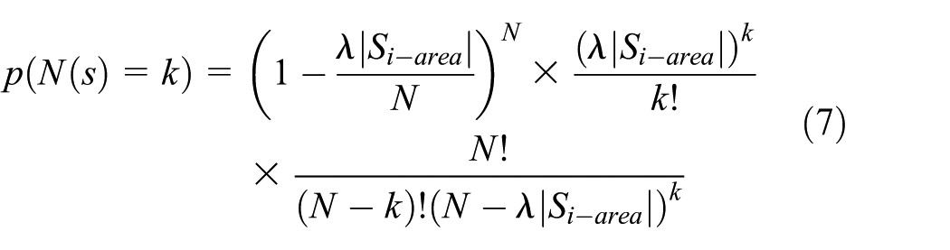
Suppose that S_i-area is the coverage area of any sensor node in the monitoring area and that S is the area of a square monitoring area whose length is l. p is the coverage probability of any sensor node in the monitoring area, that is, p = |S_i-area|/S. According to the binomial theorem and in the monitoring area, the joint probability of k sensor nodes will be

p (N (s) = k) = C_{N}^{k} p^{k} {(1 - p)}^{N - k}

(5)

Regarding the whole monitoring area, the density of the sensor nodes is λ = N/S. Thus, substitute λ and p into formula (5) to obtain

p (N (s) = k) = C_{N}^{k} {(\frac{λ | S_{i - area} |}{N})}^{k} {(1 - \frac{λ | S_{i - area} |}{N})}^{N - k}

(6)

Solve it, thus

\begin{array}{l} p (N (s) = k) = {(1 - \frac{λ | S_{i - a r e a} |}{N})}^{N} \times \frac{{(λ | S_{i - a r e a} |)}^{k}}{k!} \\ \times \frac{N!}{(N - k)! {(N - λ | S_{i - a r e a} |)}^{k}} \end{array}

(7)

When the number of sensor nodes in the monitoring area approaches infinity, that is, when N → ∞

p (N (s) = k) = \frac{e^{- λ | S_{i - area} |} {(λ | S_{i - area} |)}^{k}}{k!}

(8)

According to theorem 1, the sensor nodes randomly deployed in the monitoring area exhibit mutual independence and a uniform distribution relationship. The deployment of the number of sensor nodes obeys the probability density λ, and N(s) is the Poisson distribution of the random variable.

The random deployment model of the sensor nodes mainly addresses the problem of the distribution density of the sensor nodes.^19–21 How to use the fewest sensor nodes to complete effective coverage of the monitoring area depends on the number of sensor nodes deployed in the monitoring area at random. When there are sufficient sensor nodes deployed in a specific monitoring area, complete coverage cannot be reached; however, it is impractical from the point of node energy consumption and node redundancy. When there are many sensor nodes in the monitoring area, one node will consume substantial sensor node energy, which has no benefit for extending network life; even when the energy of a specific sink node is consumed, the whole network system will rapidly collapse. Moreover, because of the existence of many sensor nodes, a substantial number of redundant nodes will be produced during connection of the sensor nodes, and the existence of these redundant nodes will cause interference to the wireless channel, as well as consume the energy of the redundant nodes and reduce the lifetime of the network.

To overcome these two shortages, network service should be improved to a better level, and the lifetime of the network should be extended as long as possible to complete effective coverage of the monitoring area, which will improve the coverage rate of the whole monitoring area. Thus, this article introduces corollary 1.

Corollary 1

In the monitoring area, the coverage rate of the joint coverage of the sensor nodes is $p = 1 - e^{- λ {π R}_{s}^{2}}$ .

Proof

The coverage rate of any target node that is not covered by the sensor nodes is

p_{u} = \frac{e^{- λ | S_{i - area} |} {(λ | S_{i - area} |)}^{k}}{k!} \times 1 - {(\frac{| S_{i - area} |}{S})}^{k}

(9)

After the calculation

p_{u} = e^{- λ π R_{s}^{2}}

(10)

Thus, in the monitoring area, the coverage rate of joint coverage is $p = 1 - e^{- λ {π R}_{s}^{2}}$ .

The coverage quality and protocol

Redundancy coverage

In the process of covering the monitoring area and meeting a specific coverage rate, to improve the coverage quality to a better level, reduce network energy consumption, and extend the life of the network to the maximum limit, as well as to effectively schedule the work of the sensor nodes in the monitoring area, as long as the focused nodes enter the coverage hole, coverage will be degraded. To avoid hole production and complete the maximum coverage area with the fewest sensor nodes, that is, in the monitoring area, real-time monitoring of the whole monitoring area is not required; rather, coverage of the focused target nodes is required. When there are several nodes that work together and all of the Euler distances between any two nodes are smaller than or equal to the perceived radius, there will be many redundant nodes; thus, only through the dispatching schema of a node are some redundant nodes closed; when they are awoken again, the coverage rate of the redundant nodes complete coverage of the target nodes only after specific conditions are met.^6,22,23 Thus, when redundant nodes are transformed to working nodes, if the coverage rate of the redundant node did not reach the minimal value, the redundant node will go to sleep. As for the target nodes in the monitoring area, the random movements of the target nodes will make a specific sensor node cover a specific target node several times, and the value of the expected coverage value of the target node depends on the proportional relationship of the coverage rate with the movement of the target.

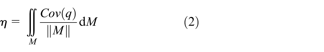
According to definition 1, the proportion that point q in monitoring area M is covered is P{1 ≥ I(q) ≥ I_th}. According to definition 2, the expected value of the coverage quality η is

E [η] = E [\int \int_{M} Cov (q) dM] . | | M | |^{- 1} = P {1 \geq I (q) \geq I_{th}}

(11)

To make the coverage qualities of the monitoring area M meet the requirement of the specified coverage quality, the only requirement is that E[η] ≥ η₀, that is

P {1 \geq I (q) \geq I_{th}} \geq η_{0}

(12)

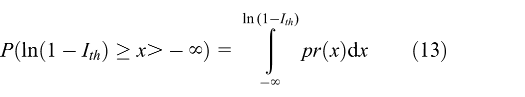
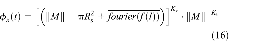
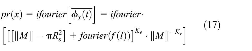
If ln(1 − I(q)) = x, then P{1 ≥ I(q) ≥ I_th} =P{ln(1 − I_th) ≥ x > −∞}, and pr(x) is used to represent the probability density function of the random variable, x, thus

P (\ln (1 - I_{th}) \geq x > - \infty) = \int_{- \infty}^{\ln (1 - I_{th})} pr (x) d x

(13)

K_v nodes in the monitoring area will be selected at random, and according to formula $x \sum_{j = 1}^{K_{v}} \ln (1 - I (s_{j}, q))$ , the characteristic function of the random variable x is

ϕ_{x} (t) = E [\exp (itx)] = E [Π_{j = 1}^{K_{v}} \exp (it \cdot \ln (1 - I (s_{j}, q)))]

(14)

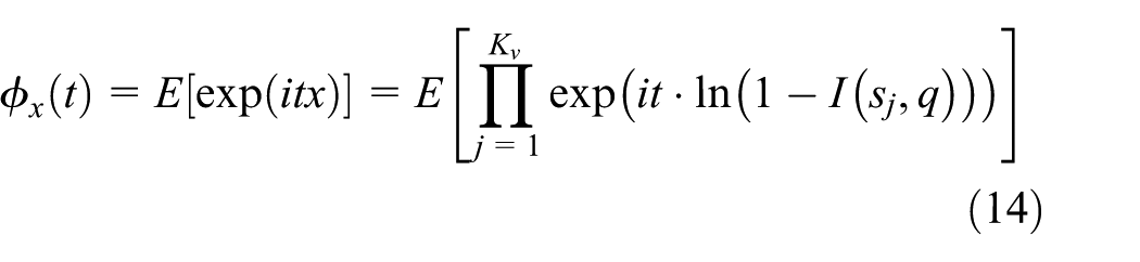
i is the imaginary unit. All of the nodes in monitoring area M comply with uniform distribution at random; thus, the proportion of a node being located at any position in the monitoring area is 1/||M||, and the positional relationships of all of the nodes in the monitoring area M are mutually independent; thus

\begin{array}{l} ϕ_{x} (t) = \\ {[‖ M ‖ - π R_{s}^{2}] + \int_{0}^{R_{s}} \exp (i t \cdot \ln (1 - \exp (- α r) \cdot 2 π r d r))}^{K_{v}} \cdot {‖ M ‖}^{- K_{v}} \end{array}

(15)

When ln(1 − exp(−αr)) = l, then

ϕ_{x} (t) = {[(‖ M ‖ - π R_{s}^{2} + \bar{fourier (f (l))})]}^{K_{v}} \cdot ‖ M ‖^{- K_{v}}

(16)

and $f (l) = (2 π \ln (1 - \exp (l) \exp (l))) / (- α^{2} (1 - \exp (l))) (1 - u (l - \ln (1 - \exp (- α R_{s}))))$ , $u (l) = {\begin{matrix} 0 l < 0 \\ 1 l > 0 \end{matrix}$ . Thus, pr(x), the probability density function of the random variable x, may be represented as

\begin{array}{l} p r (x) = i f o u r i e r [\bar{ϕ_{x} (t)}] = i f o u r i e r \cdot \\ [{[[‖ M ‖ - π R_{s}^{2}] + f o u r i e r (f (l))]}^{K_{v}} \cdot {‖ M ‖}^{- K_{v}}] \end{array}

(17)

According to formulas (13), (14), and (17)

\int_{- \infty}^{\ln (1 - I_{th})} ifourier [{[[‖ M ‖ - π R_{s}^{2}] + fourier (f (l))]}^{K_{v}} \cdot {‖ M ‖}^{- K_{v}}] d x \geq η_{0}

(18)

To ensure the establishment of formula (18), K_v working nodes are selected at random to ensure that the coverage quality of monitoring area M meets the requirement of the specific coverage quality. Moreover, the minimal value of K_v is used to establish formula (18). When the binary perception model is adopted and the boundary effect is not taken into consideration, the relationship of the expected value of the coverage quality with the number of the working nodes, K_v is $E [η] = 1 - [1 - π r_{s}^{2} / ‖ M ‖]^{K_{vb}}$ . r_s is calculated according to formula $E [η] = 1 - [1 - π r_{s}^{2} / ‖ M ‖]^{K_{vb}}$ . According to formula $1 - [1 - π r_{s}^{2} / ‖ M ‖]^{K_{vb}} \geq η_{0}$ and the least number of working nodes, K_v can be calculated, which is required to guarantee the coverage quality. Table 1 indicates that when the length of monitoring area M is 100 m long, the number of working nodes is determined by adopting the joint perception model (R_s = 10 m) as well as the binary perception model. Thus, the coverage quality can be guaranteed.

Table 1.

Parameters of the simulation table.

Parameter	Value	Parameter	Value	Parameter	Value
Monitoring area I	100 × 100	R	10 m	ε_amp	100 (J/b)/m²
Monitoring area II	200 × 200	E_R-elec	50 J/b	e_min	0.005 J
Monitoring area III	300 × 300	E_T-elec	50 J/b	Initial energy	2 J
R	5 m	ε_fs	10 (J/b)/m²	Time	100 ms

Definition 5

For a specified sensor node s_i, the specific value of the area of the perceived range that occupies the whole monitoring area is referred to as the redundant coverage rate of node s_i.

Theorem 2

Considering the triple square monitoring area as the research object, the mathematical expectation of the area that must be focused on is E(X) = np₁, and the variance is D(X) = np₁(1 − p₁). The mathematical expectation of the target area is E(Y) = np₂, and the variance is D(Y) = np₂(1 − p₂). p₁ is the coverage rate of monitoring area I, and the p₂ is that of the monitoring area II.

Proof

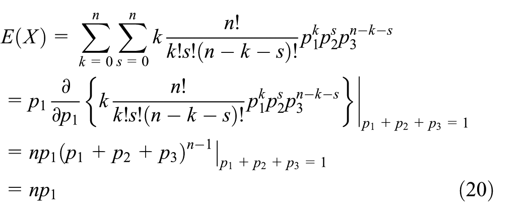
As indicated in Figure 1, for the whole target coverage area, suppose that there are n sensor nodes that complete effective coverage of the area, and monitoring area I is covered by k sensor nodes. Moreover, monitoring area II is covered by s sensor nodes, and the number of sensor nodes in monitoring area III is n − k − s. According to the subject meaning, the three monitoring areas are mutually independent, that is, the coverage rate of monitoring area III is p₃ = 1 − p₁ − p₂. The number of nodes that p₁ and p₂ cover in the monitoring area composes the discrete type random variable, which is (X, Y), and the coverage probability is

P {X = k, Y = s} = \frac{n!}{k! s! (n - k - s)!} p_{1}^{k} p_{2}^{s} p_{3}^{n - k - s}

(19)

Figure 1.

Multiple coverage.

For p₁, the expected value of the coverage probability is

\begin{matrix} E (X) = \sum_{k = 0}^{n} \sum_{s = 0}^{n} k \frac{n!}{k! s! (n - k - s)!} p_{1}^{k} p_{2}^{s} p_{3}^{n - k - s} \\ = p_{1} \frac{\partial}{\partial p_{1}} {{k \frac{n!}{k! s! (n - k - s)!} p_{1}^{k} p_{2}^{s} p_{3}^{n - k - s}} |}_{p_{1} + p_{2} + p_{3} = 1} \\ = n p_{1} {{(p_{1} + p_{2} + p_{3})}^{n - 1} |}_{p_{1} + p_{2} + p_{3} = 1} \\ = n p_{1} \end{matrix}

(20)

Moreover, the tolerance of p₁, D(X), is

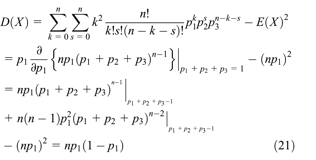
\begin{matrix} D (X) = \sum_{k = 0}^{n} \sum_{s = 0}^{n} k^{2} \frac{n!}{k! s! (n - k - s)!} p_{1}^{k} p_{2}^{s} p_{3}^{n - k - s} - E {(X)}^{2} \\ = p_{1} \frac{\partial}{\partial p_{1}} {{n p_{1} {(p_{1} + p_{2} + p_{3})}^{n - 1}} |}_{p_{1} + p_{2} + p_{3} = 1} - {(n p_{1})}^{2} \\ = {n p_{1} (p_{1} + p_{2} + p_{3})^{n - 1}}_{|_{p_{1} + p_{2} + p_{3} - 1}} \\ + {n (n - 1) p_{1}^{2} {(p_{1} + p_{2} + p_{3})}^{n - 2}}_{|_{p_{1} + p_{2} + p_{3} - 1}} \\ - {(n p_{1})}^{2} = n p_{1} (1 - p_{1}) \end{matrix}

(21)

In the same way, formula E(Y) = np₂ can be acquired, and the variance is D(Y) = np₂(1 − p₂).

Theorem 3

k working nodes are selected at random in monitoring area M; thus, the expected value of the coverage probability of M is

E (η_{k}) = 1 - {1 - \frac{π (R_{0}^{2} + σ^{2})}{area ‖ M ‖}}^{k}

(22)

Proof

The nodes in area M comply with random uniform distribution; thus, the proportion of a node in any part of area M is 1/area||M||. Any one point q in area M is covered by a sensor node a (the perceived radius of point a is R_a). Moreover, it must be located in the circle ε(q, R_a), the center of which is o and the radius of which is R_a; thus, the probability of point a being covered by q is

P_{a} = \frac{area (ε (q, R_{a}))}{area ‖ M ‖}

(23)

Because the perceived radius of point a, R_a, complies with the normal distribution N (R₀, σ²) and R₀ ≥ 3.3σ, the probability of any point of area M covered by a working node is

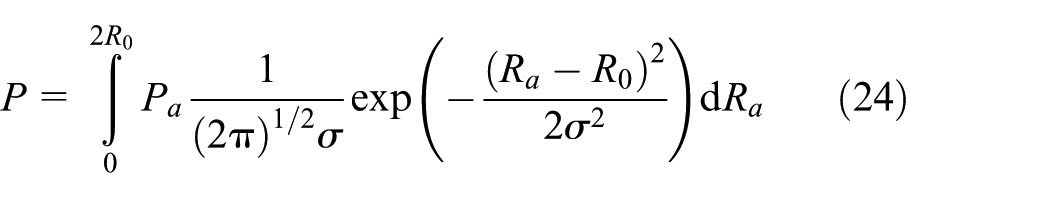
P = \int_{0}^{2 R_{0}} P_{a} \frac{1}{{(2 π)}^{1 / 2} σ} \exp (- \frac{{(R_{a} - R_{0})}^{2}}{2 σ^{2}}) d R_{a}

(24)

and $x = R_{a} - R_{0} / σ$ ; thus

\begin{matrix} P & = \frac{1}{area ‖ M ‖} {(\frac{π}{2})}^{1 / 2} (\int_{- \frac{R_{0}}{σ}}^{\frac{R_{0}}{σ}} σ^{2} x^{2} \exp (- \frac{x^{2}}{2}) d x + \int_{- \frac{R_{0}}{σ}}^{\frac{R_{0}}{σ}} 2 σ x R_{0} \exp (- \frac{x^{2}}{2}) d x + \int_{- \frac{R_{0}}{σ}}^{\frac{R_{0}}{σ}} R_{0}^{2} \exp (- \frac{x^{2}}{2}) d x) \\ \approx \frac{π (R_{0}^{2} + σ^{2})}{area ‖ M ‖} \end{matrix}

(25)

Because the positions of all of the nodes in area M are mutually independent, the probability of any node in area M being covered by at least k working nodes is

P_{k} = \sum_{i = 1}^{k} (\begin{matrix} k \\ j \end{matrix}) P^{i} {(1 - P)}^{k - i} = 1 - {(1 - \frac{π (R_{0}^{2} + σ^{2})}{area ‖ M ‖})}^{k}

(26)

Suppose that the area covered by one of the k working nodes is M_k, and the expected area of M_k is

E (area (M_{k})) = P_{k} area (M)

(27)

Thus

E (η_{k}) = \frac{E (area (M_{k}))}{area (M_{k})} = 1 - {(1 - \frac{π (R_{0}^{2} + σ^{2})}{area ‖ M ‖})}^{k}

(28)

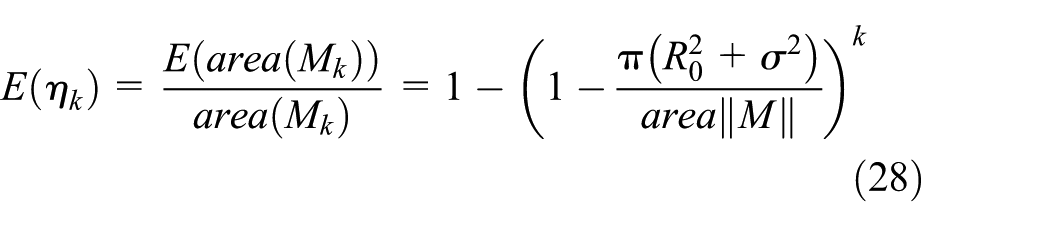
According to theorem 1, the expected minimal number of sensor nodes that meet the coverage quality, η_d, is

E (k) = \frac{\ln (1 - η_{d})}{\ln (1 - \frac{π (R_{0}^{2} + σ^{2})}{area ‖ M ‖})}

(29)

Theorem 4

After closing the redundant nodes, if the remaining working nodes accurately meet the coverage quality, then the expected number of redundant nodes, n, is

E (n) > \frac{(\ln (1 - η_{d}))}{\ln (1 - \frac{π (R_{0}^{2} + σ^{2})}{area ‖ M ‖} - 1) \cdot \frac{4 π R_{0}^{2} + 2 π σ^{2}}{area ‖ M ‖}}

(30)

Proof

Supposing that the left number of working nodes is N after closing the redundant nodes; then, these N working nodes continue to meet the random uniform distribution. Because the left working nodes meet the coverage quality, according to formula (29)

E (N) = \frac{\ln (1 - η_{d})}{\ln (1 - \frac{π (R_{0}^{2} + σ^{2})}{area ‖ M ‖})}

(31)

R_a expresses the perceived radius of node a, and R_b is the perceived radius of node b. If b is the neighboring coverage of a, then point b is locating in circle ε(a, R_a+R_b), the center of which is point a and the radius of which is R_a + R_b; thus, the probability of point b being the neighboring coverage node of point a is

P_{b - a} = \frac{area (ε (a, R_{a} + R_{b}))}{area ‖ M ‖}

(32)

Because the perceived radius of all of the nodes comply with the normal distribution, N (R₀, σ²), and R₀ ≥ 3.3σ, the probability of a node being the neighboring coverage node of another node is

P = \int_{0}^{2 R_{0}} \int_{0}^{2 R_{0}} P_{b - a} \frac{1}{2 π σ^{2}} \exp [- \frac{{(R_{a} - R_{b})}^{2} + {(R_{b} - R_{0})}^{2}}{2 σ^{2}}] \cdot d R_{a} d R_{b}

(33)

According to the calculation of formula (33)

\int_{0}^{2 R_{0}} \int_{0}^{2 R_{0}} 2 π R_{a}^{2} \frac{1}{2 π σ^{2}} \cdot \exp [- \frac{{(R_{a} - R_{b})}^{2} + {(R_{b} - R_{0})}^{2}}{2 σ^{2}}] \cdot d R_{a} d R_{b} \approx π (R_{0}^{2} + σ^{2})

(34)

and because

\begin{array}{l} \int_{0}^{2 R_{0}} R \frac{1}{{(2 π)}^{1 / 2} σ} \exp [- \frac{{(R - R_{0})}^{2}}{2 σ^{2}}] d R \\ = \int_{- \frac{R_{0}}{σ}}^{\frac{R_{0}}{σ}} (R_{0} + σ x) \frac{1}{{(2 π)}^{1 / 2}} \exp [- \frac{x^{2}}{2}] d x = R_{0} \end{array}

(35)

Thus

\int_{0}^{2 R_{0}} \int_{0}^{2 R_{0}} 2 π R_{a} R_{b} \frac{1}{2 π σ^{2}} \cdot \exp [- \frac{{(R_{a} - R_{b})}^{2} + {(R_{b} - R_{0})}^{2}}{2 σ^{2}}] \cdot d R_{a} d R_{b} = 2 π R_{0}^{2}

(36)

Hence

P = \frac{4 π R_{0}^{2} + 2 π σ^{2}}{area ‖ M ‖}

(37)

E (n) = (E (N) - 1) P = \frac{\ln (1 - η_{d})}{\ln (1 - \frac{π (R_{0}^{2} + σ^{2})}{area ‖ M ‖} - 1) \cdot \frac{4 π R_{0}^{2} + 2 π σ^{2}}{area ‖ M ‖}}

(38)

Thus, the number of working neighboring coverages of redundant nodes meets

E (n) > \frac{\ln (1 - η_{d})}{\ln (1 - \frac{π (R_{0}^{2} + σ^{2})}{area ‖ M ‖} - 1) - 1 \cdot \frac{4 π R_{0}^{2} + 2 π σ^{2}}{area ‖ M ‖}}

(39)

Definition 6

The sending intensity of any sensor node s in point a is

I = {\begin{matrix} e^{- α d_{(s, a)}} & 0 < d_{(s, a)} \leq r \\ 0 & r < d_{(s, a)} \end{matrix}

(40)

d _(s,a) is the Euclidean distance of sensor node s to any point a, α is the physical parameter of sensory mapping, and r is the perceived radius of sensor nodes. Supposing that the set of the federated nodes is T, the sensing intensity in any point a is

I (T, a) = 1 - \underset{s_{i} \in T}{Π} (1 - I (s_{i}, a))

(41)

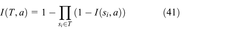
The expression of formula (41) is similar to that of any target node covered by at least one of n perceived neighboring nodes, and Sun et al.¹ and Meng et al.¹² provide the relevant proofs. Thus, in the monitoring area, the sensing intensity of a point may be described by the expression of the coverage probability of any point. This occurs because the equation of sensor nodes deployed in the monitoring area expresses randomness. When the focused moving target nodes are covered by federated nodes or single nodes, identification of the sizes of their sensing identity to improve the effectiveness of the coverage area has been suggested. Thus, this article introduces theorem 5.

Theorem 5

In the sensing range, the sensing intensity of the federated nodes is higher than that of the neighboring nodes.

Proof

Suppose that when the federated nodes cover moving target nodes, the sensing intensity is c; moreover, when the moving target nodes are covered by single nodes, the sensing intensity is w. In the sensing range, when the moving target nodes are covered by the federated nodes for the first time, the sensing intensity is c₁, and the sensing intensity of the moving target nodes that are not covered by the federated nodes, but are covered by single nodes, is w₁(1 − c₁). The second time, the probabilities of the moving target nodes being covered by the federated nodes and single nodes are C_i and W_i

C_{2} = c_{2} (1 - c_{1}) (1 - w_{1})

(42)

W_{2} = w_{2} (1 - c_{1}) (1 - w_{1}) (1 - c_{2})

(43)

When mth coverage is completed, the sensing intensities of the federated nodes and single nodes are

C_{m} = \sum_{i = 1}^{m} c_{m} Π_{i = 1}^{m - 1} (1 - c_{i}) (1 - w_{i})

(44)

W_{m} = \sum_{i = 1}^{m} w_{m} (1 - w_{m}) Π_{i = 1}^{m - 1} (1 - c_{i}) (1 - w_{i})

(45)

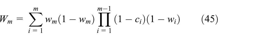
Because the positions of any sensor nodes are the same and their probabilities are events of equal probability, the sensing intensities are the same, that is, c₁ = c₂ = … = c_m; w₁ = w₂ = … = w_m, according to the geometric series theorem

C_{m} = c \frac{1 - {[(1 - c) (1 - w)]}^{m}}{1 - (1 - c) (1 - w)}

(46)

W_{m} = w (1 - c) \frac{1 - {[(1 - c) (1 - w)]}^{m}}{1 - (1 - c) (1 - w)}

(47)

When m → ∞, simplify formulas (46) and (47)

C = \frac{c}{1 - (1 - c) (1 - w)}

(48)

W = \frac{w (1 - c)}{1 - (1 - c) (1 - w)}

(49)

Because the coverage area of the federated nodes is larger than that of the single nodes, C > W, that is

c > 1 - \frac{1}{1 + w}

(50)

According to the probability theory, q∈[0, 1] when the target nodes are covered by the single nodes, that is, when w = 1, c > 1/2. Moreover, the physical meaning is that regardless of whether the target nodes are covered by the single nodes, the sensing intensity of the federated nodes occupies 50% of the total sensing intensity; thus, the sensing intensity of the federated nodes is higher than that of the single nodes.

The OCPA protocol and description

In terms of the redundancy of the sensor nodes, the redundant connected graph of the sensor nodes is established, that is, all of the nodes in the set are used to calculate the redundant information of the nodes themselves as well as their neighboring nodes according to localization, such as the received signal strength indicator (RSSI), and subsequently fuse them; the information is then sent to the sink nodes through the communication link. When the sink nodes receive redundant information, and after calculation and analysis, the redundant connected graph, G, is established according to the results of the calculation. The degree of the connected graph, G, is the number of finite sides of the relevant vertex that corresponds to the redundancy of the sensor nodes. As the number of sensor nodes increases, the redundancy will increase. In the connected graph, G, when the redundancy of the sensor nodes surpasses the threshold value that is set in advance, the sensor nodes will enter the sleeping state.²⁴ At the same time, when there are n (n > 2) high-redundant nodes in the connected graph, the high-energy nodes are chosen to be the sleeping nodes by the ranging algorithm and condition of the energy. Furthermore, the nodes and their neighboring nodes are deleted in connected graph G. The next high-energy node is subsequently found through the iterative algorithm until the redundancies of all of the sensor nodes in the connected graph are smaller than the threshold value. In terms of the energy consumption of the sensor nodes, this article manages the administrator nodes and member nodes with the help of the principle of clustering. At the initial time of the network, the member nodes send the information “inf_coverag” to the sink nodes. The information “inf_coverag” includes the location information, ID information, and energy information. After one or several rounds, when the sink nodes have received the information sent from all of the other sensor nodes, they calculate the information and subsequently store the energy of the nodes from highest to lowest in the CL; the nodes at the top of the list have higher coverage. The administrator nodes sink the sensor nodes that meet the coverage requirements in the CL according to the location information of the target nodes and send the information “inf_notice” to start effective coverage of the sensor nodes to the target nodes. Moreover, the other nodes are in a sleeping state; thus, the goal of reducing energy consumption can be attained.

1 Procedure

2 Begin

3 n ← Null //initialize the parameters

4 CL ← Null

5 While (i < n)

6 {

7 {

8 s[i].information → s[i].bata //calculate and store the information of the nodes

9 s[i].neighbor.information → s[i].neighbor.bata

10 s[i].broadcast → Gn //send the nodes to the sink nodes

11 }

12 ConstuctGraph()//set up the connected graph

13 while(s[i].energy > = minenergy)

14 if(redundancy.nodes < = I_th)//the nodes energy bigger or equal to the threshold

15 Network_working

16 else

17 {

18 sorting(s[i].energy) //ranging according to the energy

19 s[i].maxenergy → dormancy //sleeping the high-energy nodes

20 }

22 if(Gn ← s[i].inf_covergae) //the sink nodes successfully receive the node information

23 {

24 CL[i] ← s[i].inf_coverage //storing the information in the CL

25 i++//pointing to the next sensor node

26 }

27 if(s[i].energy > = s[i + 1].energy)

28 {

29 Gn.inf_notice → s[i].data //the sink nodes send the information to the nodes

30 s[i].coverage → target.nodes //the nodes covering the target nodes

31 }

32 }

Energy conversion

The OCPA algorithm uses one round of the runtime of the network as the fundamental unit, and each round includes information regarding the coverage control and information of the steady state. During the working stage, the working nodes constantly work, and all of the redundant nodes are closed to save network energy. At the steady-state stage, every node has five running states, which include the judgment, competition, standby, start-up, and sleeping states. The judgment state: at the beginning of each round, the nodes are in the judgment state.^25,26 When the nodes meet the redundant judgment requirement, they enter the sleeping state, and when the requirement is not met, the nodes will enter the competition state. The competition state: when the nodes are in the competition state, they can enter the state of the working state; otherwise, they will enter the standby state. The standby state: the nodes that fail the competition will enter the standby state; when they receive the information “on-duty” that the neighboring nodes send at the initial time and subsequently update the local information of the nodes, they will then be transferred to the judgment state. The start-up state: after the nodes successfully enter the competition state, they will enter the start-up state. When calculating the coverage probability of the nodes, it is necessary to determine whether the start-up nodes in the sensing area meet the coverage requirement; if not, the information “on-duty” will be sent and the nodes will enter the judgment state. The sleeping state: after meeting the redundant judgment, the nodes will enter the sleeping state to save energy. For each round of unit time, the nodes will be in the judgment state. The transformational relations of these five states are presented in Figure 3. When the density of the nodes in the monitoring area is too high, most of the nodes in the area will meet the judgment conditions of the redundant nodes. At this time, these nodes will enter the sleeping state, which will restrain energy consumption; however, there will be some shortage because as long as the neighboring nodes enter the sleeping state, there will be many coverage holes, which will reduce the coverage quality. To avoid this situation, the OCPA algorithm will wake up the neighboring nodes and let them enter the standby state as long as the nodes started in the sleeping state. The purpose of waking these nodes is that the density of the might-be working nodes will be reduced, and the remaining nodes will directly enter the sleeping state; any nodes awaiting working will be chosen to complete the redundant nodes schedule. Each candidate should vote itself to enter the pre-working state. Supposing that the probability is P, however, the nodes that are not successfully voted to enter the pre-working state will enter the pre-sleeping state.

1 Input N, R, r, ε

2 Initialize the number of nodes, communication radius and perception radius, threshold value

3 for i = 1 to N do

4 if coverage possibility exists then

5 determine coverage and computer coverage rate//determine the coverage area

6 state_transition (nodes)//nodes state transition function

7 else

8 break

9 end if

10 end for

11 state_transition (nodes)

12 while (node energy > ε)

13 state = wait

14 If random (0, 1) > = p then

15 compete = state

16 work = compete//meet the conditions of coverage, activate the working nodes

17 else

18 wait = compete

19 end if

20 start timer T_n//T_n is next time

21 if (d < r₁&&d < r₂) then

22 state = sleep//target nods is the neighbor nodes within the overlapping range

23 else if (random (0, 1) > = p)

24 compete = state

25 work = compete//meet the conditions of coverage, activate the working nodes

26 else

27 wait = state

28 end if

29 end if

30 end while

Complexity analysis of the algorithm

When the protocol in this article sends or receives information, it utilizes single-looping measurements to complete receipt and delivery. Thus, the complexity of the algorithm in this article is O(n); however, in the process of ranging the energy of nodes, the algorithm will take the measure of nested nodes to complete the ranging of the nodes, that is, the complexity of the algorithm is O(n²). Thus, according to the previously described analysis, the complexity of the algorithm of this article is O(n²).

System evaluation

To verify the effectiveness and stability of the algorithm in this article, the MATLAB7.0 platform is selected as the simulation platform to analyze and perform experiments on the algorithm. The computer configuration adopted in this article includes the operating system WINXP and a dual-core 1.7-GHz CPU, and the memory is 2 GB. The simulation experiment deploys all of the sensor nodes at random in the monitoring area, which has radius r, and the initial energy of all of the sensor nodes is the same, that is, 2 J. d is the distance between the communication model and communication neighboring node. Moreover, the communication of the delivery and receipt of the data is

\begin{array}{l} E_{T r} (k, d) = E_{T - e l e c} k + E_{a m p} (k, d) \\ = {\begin{matrix} E_{T - e l e c} k + ε_{f s} d^{2} k, d < d_{0} \\ E_{T - e l e c} k + ε_{a m p} d^{4} k, d \geq d_{0} \end{matrix} \end{array}

(51)

The model of the energy consumption of the receiver is

E_{Rx} (l) = E_{R - elec} (l) = l E_{elec}

(52)

E_T-elec is the energy consumption of the transmitter; E_R-elec is the energy consumption of the receiver; ε_fs is the parameter of the energy consumption of the free zone model; ε_amp is the parameter of the energy consumption of the multiple attenuation; d₀ is the distance of the communication nodes, which is referred to as the proportional amount of steel; and k is the number of nodes in the communication nodes, and the values of energy consumption are 2 and 4 when the nodes are sending or receiving data, respectively. The simulation parameters are shown in Table 1.

Figures 2 –7 indicate the changing curves of four working nodes that occupy the total number of sensor nodes under different coverage probabilities when the values of k are the same. In Figures 2 and 3, at the initial time, when the total number of sensor nodes is between 200 and 300, the speeds of the four curves rapidly increase because the value of k is smaller; thus, the number of required sensor nodes is relatively larger, but the coverage probability has not reached 99.99%; when the number is >350, the four curves tend to be steady; when the values of k are the same, for the curves with a high coverage probability, the number of working nodes is more than required; thus, the curves that have higher coverage probabilities lie at the top, whereas the lower ones lie at the bottom. In Figures 4 and 5, the four curves tend to be steady because the value of k is higher than that of the two previously described situations; for the curves that have lower coverage probabilities, the number of working nodes is 180–240. For the curves with higher coverage probabilities, the number of working nodes is 220–240, which indicates that the OCPA protocol in this article has scalability. In general, the coverage speeds of Figures 4 and 5 are higher than those of Figures 2 and 3; for the same coverage probability, the number of working nodes that Figures 4 and 5 require is smaller than that of Figures 2 and 3. Thus, the effectiveness of the algorithm in this article has been verified. Figures 6 and 7 reflect the contracting curves of the coverage probability of the OCPA protocol with the sparse conditional constant propagation (SCCP)²⁷ algorithm and compression control protocol (CCP)²⁸ algorithm in different monitoring areas of 200 × 200 m² and 300 × 300 m², respectively, when the values of k are not the same. In Figure 6, the changing curves of the coverage probability of the SCCP algorithm and CCP algorithm are between k = 1.4 and k = 1.6, which indicates that when k ≤ 1.4, the number of required sensor nodes is higher than that of the SCCP algorithm and CCP algorithm, and when k ≥ 1.6, the number of required sensor nodes is smaller than that of the SCCP algorithm and CCP algorithm because the number of redundant nodes is decreasing, which causes the number of required working nodes to decrease in the monitoring area. However, changes of parameter k do not substantially influence the number of sensor working nodes. For larger values of k, fewer required sensor nodes than needed for the SCCP algorithm and CCP algorithm may complete effective coverage. With the increase in the monitoring area, parameter k has a greater influence on the number of sensor working nodes, as shown in Figure 7; with the increase in the monitoring area, the number of sensor working nodes also increases. However, the number of working sensor nodes that the SCCP algorithm requires exceeds that of the sensor working nodes when k = 1.6, which indicates that in a larger monitoring area, the value of parameter k has a more substantial influence on the number of working sensor nodes. Thus, the coverage performance of the OCPA algorithm in this article may be strengthened under the function of the different values of parameter k.

Figure 2.

k = 1.4, the number of nodes and working nodes.

Figure 3.

k = 1.6, the number of nodes and working nodes changes graph.

Figure 4.

k = 1.8, the number of nodes and working nodes changes graph.

Figure 5.

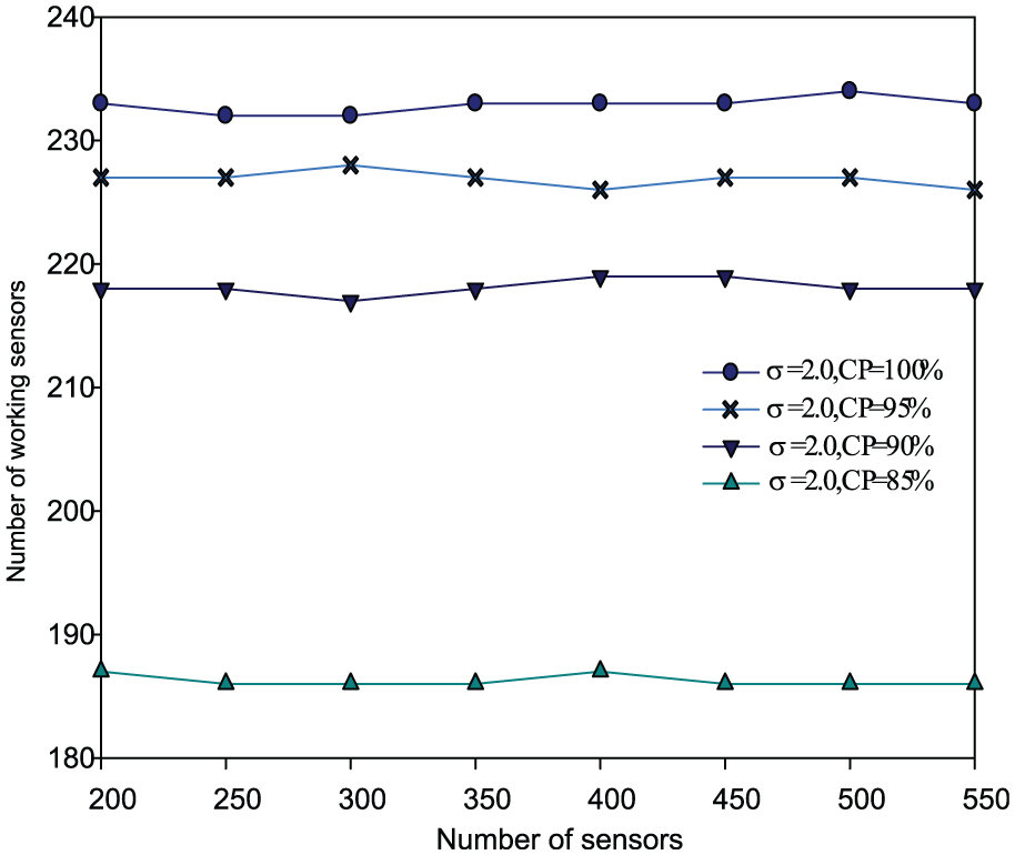
k = 2.0, the number of nodes and working nodes changes graph.

Figure 6.

200 × 200 m², comparison of the coverage probabilities of different algorithms.

Figure 7.

300 × 300 m², comparison of the coverage probabilities of different algorithms.

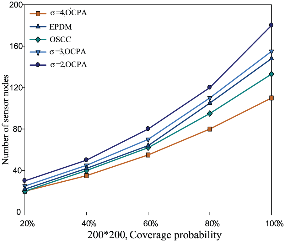
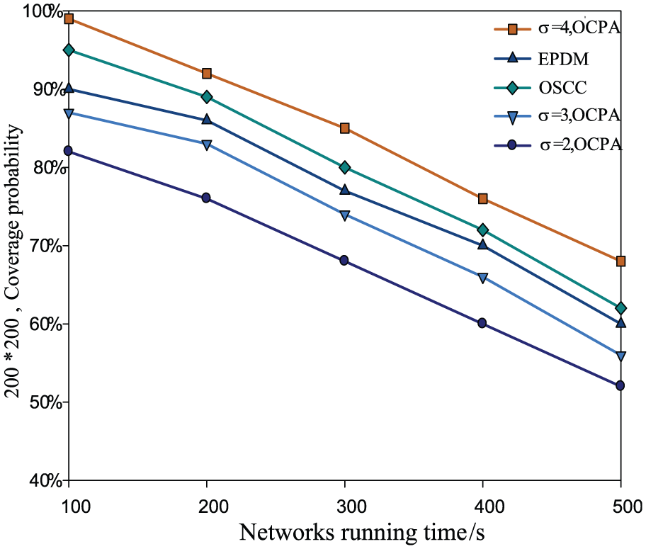
Figures 8 –11 show the contract experiments of the OCPA protocol with the energy-efficient target coverage algorithm (ETCA)²⁹ and LP_MLCEH protocol³⁰ in terms of the network lifetime in different monitoring areas. In the experiments, the values of k are different. The changes of the number of nodes deployed at random in the monitoring area change the network scale. For a smaller monitoring area, the initial number of nodes randomly deployed is 20 and increases 20 × 20. From the simulation graph, the lifetime of the wireless sensor network shows that the trance rises linearly with the increase in the number of sensor nodes because the member nodes in the node set cover the target nodes by repeatedly using the scheduling mechanism. Thus, the lifetime of the network is extended. In the same network environment, the lifetime of the OCPA protocol is prolonged 13.71% and 16.52% compared with the ETCA and LP_MLCEH protocol, respectively. For a larger monitoring area, the initial number of nodes that are randomly deployed is 50 and increases 50 × 50. The changing curves of the network lifetime tend to increase with the increase in the number of sensor nodes; however, the magnitude is smaller than that of the small monitoring area. Moreover, compared with the ETCA and LP_MLCEH protocol, the network lifetimes are prolonged by 15.13% and 17.27%, respectively. With the increase in the number of sensor nodes, the coverage probabilities of the three algorithms also tend to increase. When the coverage probability is 99.99%, k = 2, and the number of sensor nodes is 185; when k = 3, the number of sensor nodes is 152; when k = 4, the number of sensor nodes is 107, and the coverage probability of the protocol in this article reaches 99.99%, that is, complete coverage has been achieved. However, the coverage probabilities of the EPDM algorithm¹⁰ and OCPA protocol have not reached 100%. Thus, the coverage probability of the OCPA protocol in this article is higher than that of the EPDM algorithm and OCPA protocol, which verifies the effectiveness of the protocol in this article. In Figure 12, at the initial time, the coverage probabilities of the two algorithms are approximately at the same level. However, over time, the coverage probabilities of the two algorithms exhibit a decreasing trend because the EPDM algorithm and OCPA protocol adopt uninterrupted coverage of the sensor nodes during the running time. Thus, the target nodes are constantly covered until the energy of the nodes is consumed. When k = 2, 3, and 4, the coverage probabilities of the algorithms are as follows: CP_OCPA2 = 75.11%, CP_OCPA3 = 82.90%, CP_EPDM = 87.28%, CP_OSCC = 95.24%, and CP_OCPA4= 96.65%. When k = 4, the coverage probability of the OCPA protocol is higher than that of the EPDM algorithm and OCPA protocol. Thus, the coverage probability of the OCPA protocol in this article is higher than that of the other two algorithms under the function of the same node, which verifies the effectiveness of the OCPA protocol in this article. Figure 13 provides contract changing curves of the number of working nodes of the OCPA protocol compared with that of the other two algorithms when the coverage probabilities are the same. When the number of sensor nodes is maintained between 140 and 180, the numbers of working sensor nodes of the three algorithms tend to be steady. When k = 2, 3, and 4, the number of working nodes that this article requires is maintained between 146, 142, and 121; however, the numbers required by the EPDM algorithm and OCPA protocol are maintained between 134 and 152 because the protocol in this article completes coverage of the monitoring area by calculating the expected coverage value of the nodes; thus, the purpose to set the form of the local nodes within the perceived range has been reached. However, the other two algorithms complete coverage of the monitoring area using constant coverage. Thus, the average number of sensor nodes that the protocol in this article requires is smaller than that of the other two algorithms, that is, it decreases by 3.49%.

Figure 8.

100 × 100 m², curves of network life.

Figure 9.

200 × 200 m², curves of network life.

Figure 10.

300 × 300, curves of network life.

Figure 11.

200 × 200, curves of network coverage.

Figure 12.

200 × 200, curves of network runtime.

Figure 13.

Curves of the sensor working nodes and sensor nodes.

Conclusion

To determine the coverage of a wireless sensor network, this article proposes an OCPA. The protocol in this article seamlessly provides a method to solve the largest coverage area of the three-circle first; moreover, taking advantage of the probability theory, this article provides the expected value of the coverage quality of the monitoring area. On this basis, this article also provides a solving method for the smallest number of sensor nodes. On the basis of analyzing the coverage probability of the nodes, this article provides the contract relationship of the sensing intensity of federated nodes and single nodes. In terms of the coverage of redundant nodes, this article proves the conditions of the redundant coverage of sensor nodes. Finally, the protocol in this article simulates the optimized deployment, coverage probability, redundancy, network lifetime, and running time, as well as analyzes the simulation results, which verified the effectiveness and feasibility of the OCPA protocol.

Footnotes

Academic Editor: Fei Yu

Declaration of conflicting interests

The author(s) declared no potential conflicts of interest with respect to the research, authorship, and/or publication of this article.

Funding

The author(s) disclosed receipt of the following financial support for the research, authorship, and/or publication of this article: This study was supported by projects 61628210 and 61503174 supported by the National Natural Science Foundation of China; projects (no. 2016GGJS-158) supported by Cultivation Young Key Teachers in Colleges and Universities of Henan; projects 17A520044 and 15A413016 supported by the Henan Province Education Department Natural Science Foundation; projects 162102210113 and 162102410051 supported by the Henan Province Department Science Natural Science and Technology Research; projects 1201430560 supported by the Guangzhou Education Bureau Science Foundation; projects 2016A030313540 supported by the Guangdong Natural Science Foundation of China; and projects 2016SF-428 supported by the Shanxi Education Bureau Science Foundation.

References

Sun

Xing

. A novel nonlinear multitarget k-degree coverage preservation protocol in wireless sensor networks. J Sens 2016; 2016(1): 3434961-1–3434961-13.

Tseng

Chen

WT.

k-Angle object coverage problem in a wireless sensor network. IEEE Sens J 2012; 12(12): 3408–3416.

Xiao

Chen

. Coverage and detection of a randomized scheduling algorithm in wireless sensor networks. IEEE T Comput 2010; 59(4): 507–521.

Ammari

Das

SK.

Centralized and clustered k-coverage protocols for wireless sensor networks. IEEE T Comput 2012; 61(1): 118–132.

Sun

Wang

. An optimized strategy coverage control algorithm for WSN. Int J Distrib Sens N 2014; 2014(3): 1–12.

Tahiry

David

SR.

Connectivity preservation and coverage schemes for wireless sensor networks. IEEE T Automat Contr 2011; 56(10): 2418–2428.

Wang

Guo

Maximizing the lifetime of k-discrete barrier coverage using mobile sensors. IEEE Sens J 2013; 13(12): 4690–4701.

Cardei

DZ.

Improving wireless sensor network lifetime through power aware organization. Wirel Netw 2005; 11(3): 333–340.

Seok

Lee

JJ.

A bipopulation-based evolutionary algorithm for solving full area coverage problems. IEEE Sens J 2013; 13(12): 4796–4807.

10.

Sun

Wang

. A novel coverage algorithm based on event-probability-driven mechanism in wireless sensor network. EURASIP J Wirel Comm 2014; 2014(1): 58.

11.

Zhao

Liu Qiang

ZL.

Optimization strategy on coverage control in wireless sensor network based on Voronoi. J Comm 2013; 34(9): 115–122.

12.

Meng

Wang

Connected coverage protocol using cooperative sensing model for wireless sensor networks. Acta Electron Sin 2011; 39(4): 772–779.

13.

Mini

Siba

Samrat

LS.

Sensor deployment and scheduling for target coverage problem in wireless sensor networks. IEEE Sens J 2014; 14(3): 636–644.

14.

Hanid

Kaveh

Amir

. Distributed deployment algorithms for improved coverage in a network of wireless mobile sensors. IEEE T Ind Inform 2014; 10(1): 163–174.

15.

. Transforming complete coverage algorithms to partial coverage algorithms for wireless sensor networks. IEEE T Parall Distr 2011; 22(4): 695–703.

16.

Zhibo

Jilong

Qing

. Achieving k-barrier coverage in hybrid directional sensor networks. IEEE T Mobile Comput 2014; 13(7): 1443–1455.

17.

Sun

Wang

. A novel energy-efficient k-coverage algorithm based on probability driven mechanism of wireless sensor networks. Int J Distrib Sens N 2016; 2016(1): 7474926-1–7474926-9.

18.

Otero

Haber

Peter

. A wireless sensor networks’ analytics system for predicting performance in On-demand deployments. IEEE Syst J 2015; 9(4): 1344–1353.

19.

Yoon

Kim

YH.

An efficient genetic algorithm for maximum coverage deployment in wireless sensor networks. IEEE T Cybern 2013; 43(5): 1473–1483.

20.

Zheng

Xiao

Wang

. Capacity and delay analysis for data gathering with compressive sensing in wireless sensor networks. IEEE T Wirel Commun 2013; 12(2): 917–927.

21.

Sun

Zhang

Xing

. EBKCCA: a novel energy balanced k-coverage control algorithm based on probability model in wireless sensor networks. KSII T Internet Inf 2016; 10(8): 3621–3640.

22.

Jin

Wang

. ECCRA: an energy-efficient coverage and connectivity preserving routing algorithm under border effects in wireless sensor networks. Comput Commun 2008; 31(10): 2398–2407.

23.

Gong

Zhang

JS.

Curve-based deployment for barrier coverage in wireless sensor networks. IEEE T Commun 2014; 13(2): 724–735.

24.

Tao

Krunz

Coverage-time optimization for clustered wireless sensor networks: a power-balancing approach. IEEE/ACM T Network 2010; 18(1): 202–215.

25.

Imran

Haider

Alnuem

. Efficient movement control actor relocation for honing connected coverage in wireless sensor and actor networks. In: Proceedings of the 2012 IEEE 37th conference on local computer networks workshops (LCN Workshops), Clearwater, FL, 22–25 October 2012, pp.710–717. New York: IEEE.

26.

Chiwewe

Hancke

GP.

A distributed topology control technique for low interference and energy efficiency in wireless sensor networks. IEEE T Ind Inform 2015; 8(1): 11–19.

27.

Xing

Wang

. Square region-based coverage and connectivity probability model in wireless sensor networks. In: Proceedings of the IEEE 5th international conference on collaborative computing networking, applications and worksharing (CollaborateCom 2009), Washington, DC, 11–14 November 2009, pp.1–8. New York: IEEE.

28.

Xing

Wang

Zhang

. Integrated coverage and connectivity configuration for energy conservation in sensor networks. ACM T Sensor Network 2005; 1(1): 36–72.

29.

Xing

Wang

Polytype target coverage scheme for heterogeneous wireless sensor networks using linear programming. Wirel Commun Mob Com 2014; 14(14): 1397–1408.

30.

Yang

Chin

KW.

Novel algorithms for complete targets coverage in energy harvesting wireless sensor networks. IEEE Commun Lett 2014; 18(1): 118–121.

Optimization coverage conserving protocol with authentication in wireless sensor networks

Abstract

Keywords

Introduction

Relative literature

Prerequisite knowledge

Definition 1

Definition 2

Definition 3

Definition 4

Theorem 1

Proof

Corollary 1

Proof

The coverage quality and protocol

Redundancy coverage

Definition 5

Theorem 2

Proof

Theorem 3

Proof

Theorem 4

Proof

Definition 6

Theorem 5

Proof

The OCPA protocol and description

Energy conversion

Complexity analysis of the algorithm

System evaluation

Conclusion

Footnotes

Declaration of conflicting interests

Funding

References