A modified truncation singular value decomposition method for solving ill-posed problems

Abstract

A modified truncated singular value decomposition method for solving ill-posed problems is presented in this paper, in which the solution has a slightly different form. Both theoretical and numerical results show that the limitations of the classical TSVD method have been overcome by the new method and very few additive computations are needed.

Introduction

The research of theories and algorithm for inverse problems is a hot topic in computational and applied mathematics. The main difficult of inverse problems is that they are usually ill-posed problems, i.e. arbitrarily small error in the input data may cause huge errors in their approximate solutions. ¹ In the past years, many methods have been reported to treat the ill-posedness of inverse problems. These works mainly fall into four categories: Tikhonov regularization methods, iteration regularization methods, mollification methods, and spectral regularization methods.^1,2 Because the spectrum of infinite dimensional compact operators is hard to calculate, spectral regularization method does not attract much attention in practical computation. However, in the process of computation, we have to discretize the problems into finite dimensions. And there are already quite mature algorithms for calculating the singular systems of finite dimensional operators.^3,4 So the spectral regularization methods deserve further attention. In this paper, we present a modified truncated singular value decomposition (mTSVD) method, which is a kind of spectral regularization method.

We consider linear operator equations of the form

$$Tx=y$$

(1)

where T is a bounded compact operator between Hilbert spaces X and Y. Instead of y, in practice, we usually only have perturbed data $y^{\delta }$ . And the condition

$$\left|\right|y^{\delta }-y\left|\right|\le \delta ,\hspace{1em}\left|\right|y^{\delta }\left|\right|>\tau \delta$$

(2)

are assumed with δ being a known error level and $\tau >1$ is a constant. The perturbed form of equation (1) is

$$Tx=y^{\delta }$$

(3)

Let ${\{{\sigma }_i,v_i,u_i\}}_{i\in N}$ is a singular system of T, where

$${\sigma }_1\ge {\sigma }_2\ge \cdots \ge {\sigma }_n\ge \cdots$$

(4)

then classical TSVD solution of equation (1) is defined as

$${\widehat{x}}^{\delta }=:{\displaystyle \sum _{i=1}^n\frac{1}{{\sigma }_i}}〈f,u_i〉v_i$$

(5)

where n is determined by

$${\displaystyle \sum _{i=n}^{\infty }{〈y^{\delta },u_i〉}^2}\le {\tau }^2{\delta }^2<{\displaystyle \sum _{i=n-1}^{\infty }{〈y^{\delta },u_i〉}^2}$$

(6)

The TSVD is commonly used to solve ill-posed problems. Hanson ⁵ have used it to solve the Fredholm integral equations of the first kind in the early stages. Hansen pointed out that the use of the TSVD has certain similarities with the use of regularization in Tikhonov form and investigated the connection between the two methods. ⁶ Hereafter, the TSVD method and its generalized forms are widely used in various ill-posed problems.^7–12

In this paper, we present a mTSVD method. The solution with a slightly different form is used in the new method and very few additive computations are needed. We have proved that the error bound of the new method is better than the old one. Moreover, we should not worry about how to choose the parameter τ in the discrepancy principle for the new method when the smoothness of the solution is greater than $\frac{1}{2}$ . Some numerical tests also verify the advantages of the new method.

This paper is organized as follows. The new method and its convergence result are presented in the next section. Then, a theoretical comparison between the new method and the classical one is presented. Then, some numerical comparisons are given to show the advantages of the new method.

The mTSVD method

The mTSVD approximation solution of equation (3) is defined as: Let ${\sigma }_0=\infty$ , and assume $g^{\delta }\ne 0$ , if there exists a nonnegative integer m such that

$${\sigma }_m>{\sigma }_{m+1}={\sigma }_{m+2}=\cdots ={\sigma }_{m+k}>{\sigma }_{m+k+1}$$

(7)

and

$${\displaystyle \sum _{i=m+k+1}^{\infty }{〈y^{\delta },u_i〉}^2}\le {\tau }^2{\delta }^2<{\displaystyle \sum _{i=m+1}^{\infty }{〈y^{\delta },u_i〉}^2}$$

(8)

then the mTSVD solution to equation (3) will be defined by

$$x^{\delta }=x_{m,\xi }^{\delta }={\displaystyle \sum _{i=1}^m\frac{1}{{\sigma }_i}}〈y^{\delta },u_i〉v_i+\xi {\displaystyle \sum _{i=m+1}^{m+k}\frac{1}{{\sigma }_i}}〈y^{\delta },u_i〉v_i$$

(9)

the value $\xi =\xi (\delta ,y^{\delta })>0$ in equation (9) is determined by the discrepancy principle

$$\left|\right|T{x}_{m,\xi }^{\delta }-y^{\delta }\left|\right|=\tau \delta$$

(10)

Remark 1. It can be derived that

$$\xi =\frac{1-{\left[{\tau }^2{\delta }^2+{\displaystyle {\sum }_{i=1}^{m+k}{〈y^{\delta },u_i〉}^2}-\left|\right|y^{\delta }|{|}^2\right]}^{\frac{1}{2}}}{{\displaystyle {\sum }_{i=m+1}^{m+k}{〈y^{\delta },u_i〉}^2}}$$

(11)

which indicate $\xi \in (0,1]$ , ξ = 1 when the equality holds in equation (8).

For the mTSVD solution of equation (3), we have the following theorem:

Theorem 2. Suppose that the condition (2) holds, $x^{\delta }$ is defined by equations (9) and (10), the best approximate solution $x^{†}=T^{†}y\in R{(T^{*}T)}^{\nu }$ , then

$$\left|\right|x^{\delta }-x^{†}\left|\right|\le C_{\tau ,\nu }{\left(\left|\right|x|{|}_{\nu }\right)}^{\frac{1}{2\nu +1}}{\delta }^{\frac{2\nu }{2\nu +1}}$$

(12)

where

$$C_{\tau ,\nu }=\left[\frac{{\alpha }_m}{{\left(\tau -\sqrt{1-{\alpha }_m^2}\right)}^{\frac{1}{2\nu +1}}}+{\left(\tau +\sqrt{1-{\alpha }_m^2}\right)}^{\frac{2\nu }{2\nu +1}}\right]$$

(13)

with

$$0\le {\alpha }_m\le 1$$

(14)

Proof. For any $w\in y$ , we define

$$M_{m,\xi }w=:{\displaystyle \sum 〈w,u_i〉}{u}_i+\xi {\displaystyle \sum _{i=m+1}^{m+k}〈w,u_i〉}{u}_i$$

(15)

and

$$R_{m,\xi }w=:T^{†}{M}_{m,\xi }w={\displaystyle \sum \frac{1}{{\sigma }_i}}〈w,u_i〉v_i+\xi {\displaystyle \sum _{i=m+1}^{m+k}\frac{1}{{\sigma }_i}}〈w,u_i〉v_i$$

(16)

Let $e=y^{\delta }-y$ and

$${\alpha }_m=:\frac{\left|\right|M_{m,\xi }e\left|\right|}{\delta }$$

(17)

It can be verified that $0\le {\alpha }_m\le 1$ . By using the triangle inequality, we know

$$\begin{array}{lll}\left|\right|x^{\delta }-x^{†}\left|\right|\hfill & =\hfill & \left|\right|x^{\delta }-R_{m,\xi }y+R_{m,\xi }y-x^{†}\left|\right|\hfill \\ \hfill & \le \hfill & \left|\right|x^{\delta }-R_{m,\xi }y\left|\right|+\left|\right|R_{m,\xi }y-x^{†}\left|\right|\hfill \\ \hfill & \le \hfill & \frac{{\alpha }_m}{{\sigma }_{m+1}}\delta +\left|\right|R_{m,\xi }y-x^{†}\left|\right|\hfill \end{array}$$

(18)

From equation (10)

$$\left|\right|(I-M_{m,\xi })y^{\delta }\left|\right|=\left|\right|y^{\delta }-T{x}^{\delta }\left|\right|=\tau \delta$$

(19)

Moreover

$$\left|\right|e|{|}^2=||(I-M_{m,\xi }e|{|}^2+|\left|M_{m,\xi }\right|{|}^2+2〈\left(I-M_{m,\xi }\right)e,M_{m,\xi }e〉$$

(20)

and

$$〈\left(I-M_{m,\xi }\right)e,M_{m,\xi }e〉=\xi (1-\xi ){\displaystyle \sum _{i=m+1}^{m+k}{〈e,u_i〉}^2}\ge 0$$

(21)

In terms of equations (17), (19), (20) and (21), we have

$$\left|\right|\left(I-M_{m,\xi })\right)\left|\right|\le \sqrt{1-{\alpha }_m^2}\delta$$

(22)

Therefore

$$\left(\tau +\sqrt{1-{\alpha }_m^2}\right)\delta \ge \left|\right|\left(I-M_{m,\xi }\right)y\left|\right|=\left|\right|\left(I-M_{m,\xi }\right)\left(y^{\delta }-e\right)\left|\right|\ge \left(\tau -\sqrt{1-{\alpha }_m^2}\right)$$

(23)

On other hand

$$\begin{array}{l}\left|\right|\left(I-M_{m,\xi }\right)y|{|}^2\\ {=\left(1-\xi \right)}^2{\displaystyle \sum _{i=m+1}^{m+k}{〈y,u_i〉}^2}+{\displaystyle \sum _{i=m+k+1}^{\infty }{〈y,u_i〉}^2}\\ ={\left(1-\xi \right)}^2{\displaystyle \sum _{i=m+1}^{m+k}{\sigma }_i^2}{〈x^{†},v_i〉}^2+{\displaystyle \sum _{i=m+k+1}^{\infty }{\sigma }_i^2}{〈x^{†},v_i〉}^2\end{array}$$

(24)

Owing to $x^{†}={(T^{*}T)}^{\nu }z$ , so we have

$$\begin{array}{c}||(I-M_{m,\xi })g|{|}^2=(1-\xi {)}^2{\displaystyle \sum _{i=m+1}^{m+k}{\sigma }_i^{4\nu +2}}〈z,v_i{〉}^2\\ +{\displaystyle \sum _{i=m+k+1}^{\infty }{\sigma }_i^{4\nu +2}}〈z,v_i{〉}^2\le {\sigma }_{m+1}^{4\nu +2}a(z,\delta {)}^2\end{array}$$

(25)

where

$$a(z,\delta )={(1-\xi )}^2{\displaystyle \sum _{i=m+1}^{m+k}{〈z,v_i〉}^2}+{\displaystyle \sum _{i=m+k+1}^{\infty }{〈z,v_i〉}^2}$$

(26)

We have

$$\underset{\delta \to 0}{\lim }a(z,\delta )=0, a(z,\delta )\le \left|\right|z\left|\right|=\left|\right|x^{†}|{|}_{\nu }$$

(27)

Combining equations (25) and (27) with equation (23), we have

$${\sigma }_{m+1}\ge {\left(\frac{\tau -\sqrt{1-{\alpha }_m^2}}{\left|\right|x^{†}|{|}_{\nu }}\right)}^{\frac{1}{2\nu +1}}{\delta }^{\frac{1}{2\nu +1}}$$

(28)

Hence

$$\frac{{\alpha }_m}{{\sigma }_{m+1}}\delta <\left|\right|x^{†}|{|}_{\nu }^{\frac{1}{2\nu +1}}\frac{{\alpha }_m}{{(\tau -\sqrt{1-{\alpha }_m^2})}^{\frac{1}{2\nu +1}}}{\delta }^{\frac{2\nu }{2\nu +1}}$$

(29)

Moreover, by using the Hólder inequality

$$\begin{array}{l}\left|\right|R_{m,\xi }y-x^{†}\left|\right|\\ ={(1-\xi )}^2{\displaystyle \sum _{i=m+1}^{m+k}{\sigma }_i^{-2}}{〈y,u_i〉}^2+{\displaystyle \sum _{i=m+k+1}^{\infty }{\sigma }^{-2}}{〈y,u_i〉}^2\\ ={(1-\xi )}^2{\displaystyle \sum _{i=m+1}^{m+k}{\sigma }_i^{4\nu }}{〈z,v_i〉}^2+{\displaystyle \sum _{i=m+k+1}^{\infty }{\sigma }^{4\nu }}{〈z,v_i〉}^2\\ \le {\left[{(1-\xi )}^2{\displaystyle \sum _{i=m+1}^{m+k}{\sigma }_i^{4\nu +2}}{〈z,v_i〉}^2+{\displaystyle \sum _{i=m+k+1}^{\infty }{\sigma }_i^{4\nu +2}}{〈z,v_i〉}^2\right]}^{\frac{2\nu }{2\nu +1}}\\ \times {\left[{(1-\xi )}^2{\displaystyle \sum _{i=m+1}^{m+k}{〈z,v_i〉}^2}+{\displaystyle \sum _{i=m+k+1}^{\infty }{〈z,v_i〉}^2}\right]}^{\frac{1}{2\nu +1}}\hfill \\ =a{(z,\delta )}^{\frac{2}{2\nu +1}}\left|\right|(I-M_{m,\xi })y|{|}^{\frac{4\nu }{2\nu +1}}\hfill \end{array}$$

(30)

Substituting equation (23) into equation (30), we obtain

$$\left|\right|R_{m,\xi }y-x^{†}|{|}^2\le a{(z,\delta )}^{\frac{1}{2\nu +1}}{\left(\tau +\sqrt{1-{\alpha }^2}\right)}^{\frac{2\nu }{2\nu +1}}{\delta }^{\frac{2\nu }{2\nu +1}}$$

(31)

The assertion of the theorem follows from equations (18), (29) and (31).

Theoretical comparison with the classical method

It is well known that the following theorem holds for the classical TSVD solution

Theorem 3 ¹³ . Suppose the conditions of theorem 1 hold, then we have

$$\left|\right|{\widehat{x}}^{\delta }-x^{†}\left|\right|\le {\widehat{C}}_{\tau ,\nu }{(|\left|x\right|{|}_{\nu })}^{\frac{1}{2\nu +1}}{\delta }^{\frac{2\nu }{2\nu +1}}$$

(32)

where

$${\widehat{C}}_{\tau ,\nu }=\left[{(\tau -1)}^{-\frac{1}{2\nu +1}}+{(\tau +1)}^{\frac{2\nu }{2\nu +1}}\right]$$

(33)

Theorem 4. By contrasting equations (13) and (33), we can obtain

1. For any $\tau >1$ and $\nu >0$ , we have

$$C_{\tau ,\nu }\le {\widehat{C}}_{\tau ,\nu }$$

(34)

2. If $\nu \ge \frac{1}{2}$ , we can let τ = 1 in equation (10) and we have

$$C_{\tau ,\nu }\le 2\sqrt{2}$$

(35)

Proof.

1. Note that $\tau >1$ , we have

$$\sqrt{1-{\alpha }_m^2}-{\alpha }_m^{2\nu +1}\le 1-{\alpha }_m^{2\nu +1}\le \tau (1-{\alpha }_m^{2\nu +1})$$

(36)

Hence

$${\alpha }_m^{2\nu +1}(\tau -1)\le \tau -\sqrt{1-{\alpha }_m^2}$$

(37)

By using the monotonicity of exponential function

$${\alpha }_m{(\tau -1)}^{\frac{1}{2\nu +1}}\le {(\tau -\sqrt{1-{\alpha }_m^2})}^{\frac{1}{2\nu +1}}$$

(38)

So we have

$$\frac{{\alpha }_m}{{(\tau -\sqrt{1-{\alpha }_m^2})}^{\frac{1}{2\nu +1}}}\le \frac{1}{{(\tau -1)}^{\frac{1}{2\nu +1}}}$$

(39)

On the other hand

$$\tau +\sqrt{1-{\alpha }_m^2}\le \tau +1$$

(40)

Therefore

$${(\tau +\sqrt{1-{\alpha }_m^2})}^{\frac{2\nu }{2\nu +1}}\le {(\tau +1)}^{\frac{2\nu }{2\nu +1}}$$

(41)

The assertion of the theorem follows from equations (39) and (41).

2. For $\nu =\frac{1}{2}$ , τ = 1, we have

$$C_{1,\frac{1}{2}}=\frac{{\alpha }_m}{{(1-\sqrt{1-{\alpha }_m^2})}^{\frac{1}{2}}}+{\left(1+\sqrt{1-{\alpha }_m^2}\right)}^{\frac{1}{2}}=:I_1+I_2$$

(42)

We now estimate I₁ and I₂ separately. If we let

$$f(\alpha )=\frac{\alpha }{{(1-\sqrt{1-{\alpha }^2})}^{\frac{1}{2}}}$$

(43)

then it can be verified that the solution of equation

$$f^{\prime }(\alpha )=0$$

(44)

are ${\alpha }_1=0$ and ${\alpha }_2=1$ . So we can get

$$I_1\le \underset{0\le \alpha \le 1}{\max }f(\alpha )=f(0)=\sqrt{2}$$

(45)

On other hand, it is obvious that

$$I_2\le {(1+1)}^{1/2}=\sqrt{2}$$

(46)

So we can get

$$C_{1,\frac{1}{2}}\le 2\sqrt{2}$$

(47)

Moreover, if ${\nu }_1\ge {\nu }_2$ , then for any fixed α_m, we have

$$C_{1,{\nu }_1}\le C_{1,{\nu }_2}$$

(48)

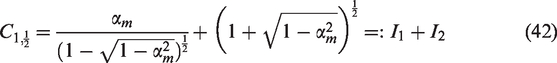
This finishes the proof of theorem 2.

Numerical comparison with the classical method

In this section, we give some numerical tests to compare the new method with the classical one. All examples are taken from the Matlab package by Hansen. ¹⁴ We take the number of nodes N = 200, $\tau =1.001$ and T, x and y are generated by the function in package. The perturbed data are given by

$$y^{\delta }(t_j)=y(t_j)+\mathrm{ϵ}\times \delta (t_j)$$

(49)

where ϵ is the level of error and $\delta (t_j)$ are generated by three means

1.

$${\delta }_1(t)=2\times \text{rand}(N)-1$$

(50)

2.

$${\delta }_2(t)=\text{randn}(N)$$

(51)

3.

$${\delta }_3(t)=\sqrt{2}\sin (20t)$$

(52)

where the Matlab functions $\text{rand}(·)$ and $\text{randn}(·)$ generate uniformly distributed and normally distributed random numbers.

Example 1

$$[\text{T},\text{y},\text{x}]\text{=deriv2}(\text{N},\text{3})$$

Example 2

$$[\text{T},\text{y},\text{x}]\text{=foxgood}(\text{N},\text{3})$$

The explanations of Matlab functions $\text{deriv2}$ and $\text{foxgood}$ can be found in package. In the following, we give the figures that the relative errors $\frac{\left|\right|{\widehat{x}}^{\delta }-x\left|\right|}{\left|\right|x\left|\right|}$ and $\frac{\left|\right|x^{\delta }-x\left|\right|}{\left|\right|x\left|\right|}$ change on ϵ, respectively. Here, the solid curve represents the relative errors of classical TSVD solution, and dotted curves indicate the relative errors of modified TSVD solution.

From the above figures, we can see that when ϵ decreases, the relative errors of the mTSVD solution almost always become smaller but the relative errors of the classical TSVD solutionis rebound in Figures 1(a) and (b) and 2(a) to (c). So we can conclude that the mTSVD method is much stable than the classical one.

Figure 1.

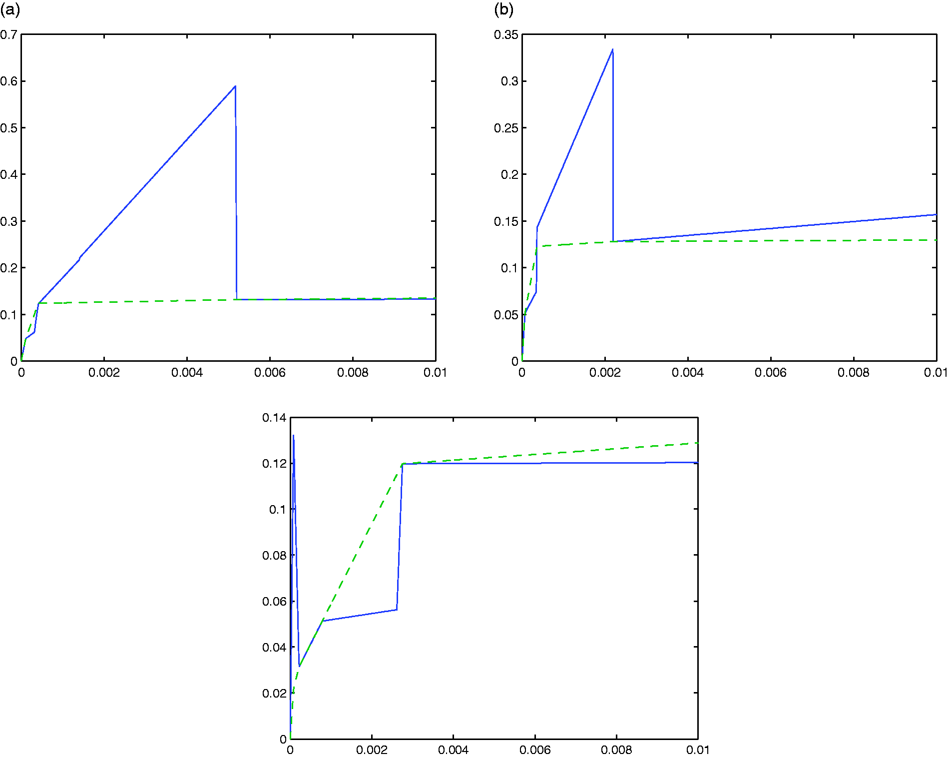
The relative errors of numerical solutions (Example 1). (a) δ₁ = 0.1, α = 1.1. (b) δ₁ = 0.01, α = 1.1. (c) δ₁ = 0.1, α = 1.5.

Figure 2.

The relative errors of numerical solutions (Example 2). (a) δ₁ = 0.1, α = 1.1. (b) δ1 = 0.01, α = 1.1. (c) δ₁ = 0.1, α = 1.5.

Conclusion

In this paper, we present a mTSVD method for solving ill-posed problems. A slight modification in form is made and very few additive computations are needed, but both theoretical and numerical results show that the new method has unique advantages than the classical one.